
Assimilating Aeolus Satellite Wind Data on a Regional Level: Application in a Mediterranean Cyclone Using the WRF Model

Abstract
:1. Introduction
2. Materials and Methods
2.1. WRF Model
2.2. WRF Data Assimilation (DA)
2.3. Aeolus
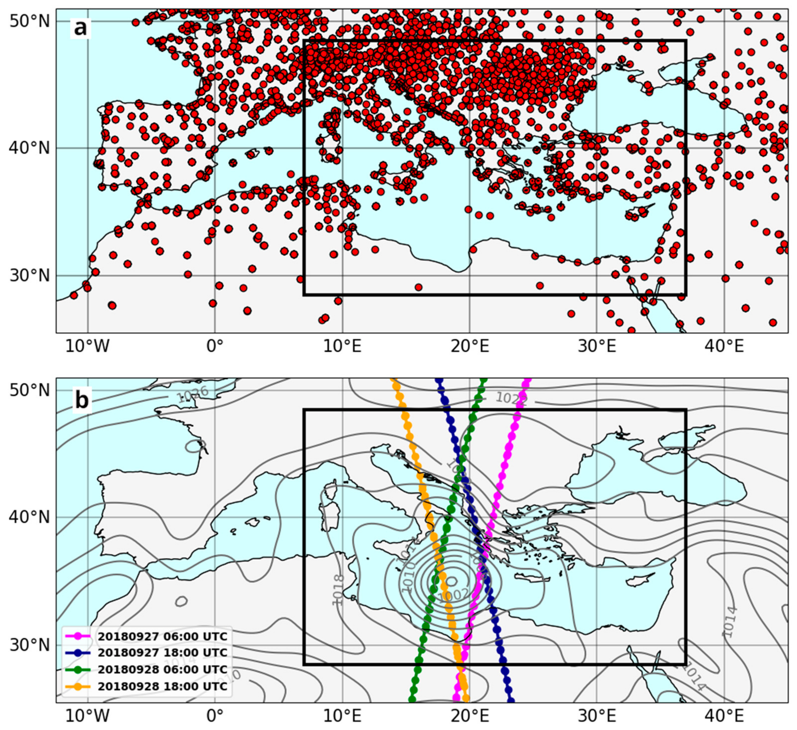
2.4. Case Study
2.5. Methodology
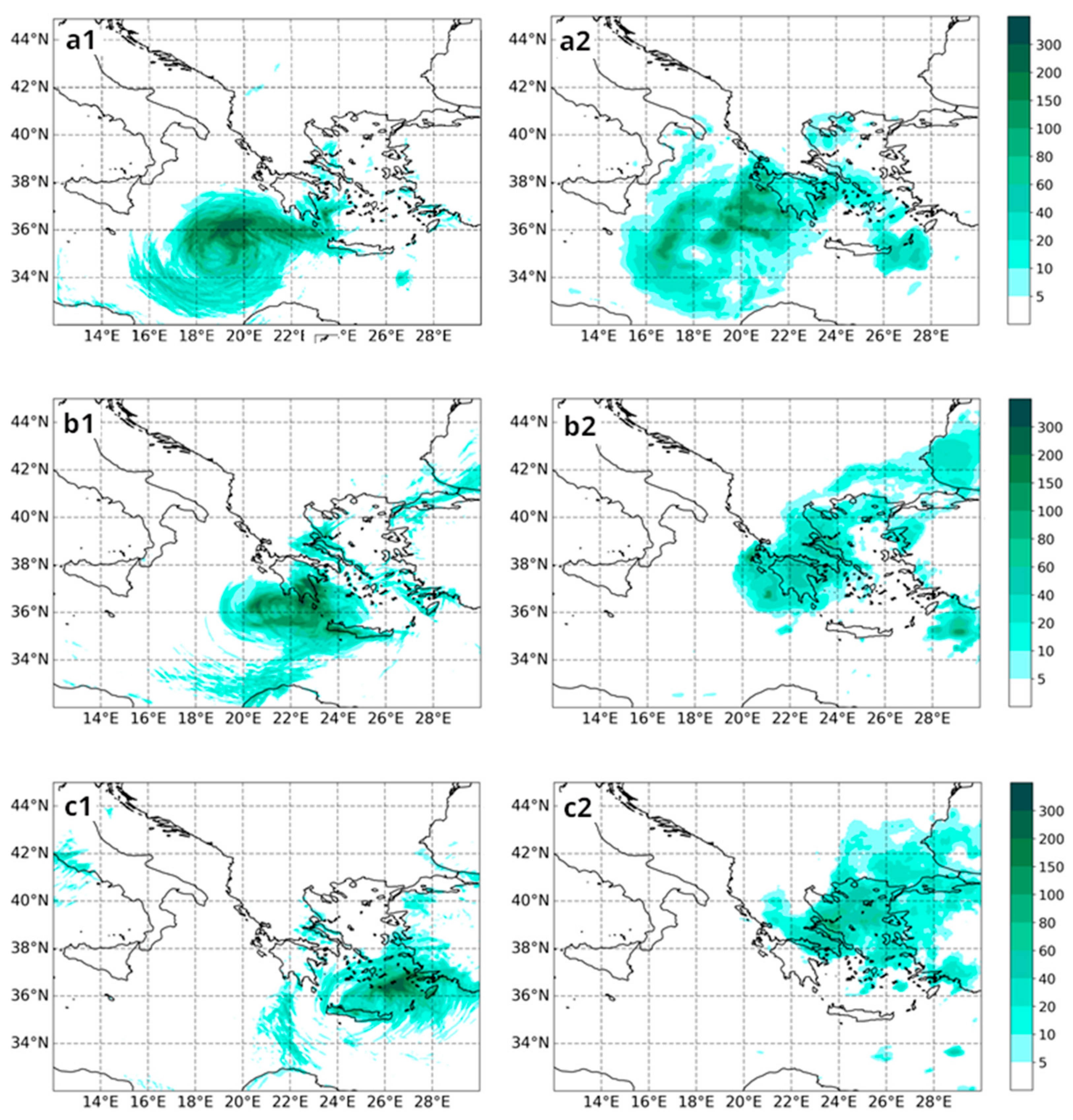
3. Results
4. Discussion and Conclusions
Author Contributions
Funding
Institutional Review Board Statement
Informed Consent Statement
Data Availability Statement
Acknowledgments
Conflicts of Interest
References
- Miglietta, M.M. Mediterranean Tropical-Like Cyclones (Medicanes). Atmosphere 2019, 10, 206. [Google Scholar] [CrossRef]
- Flaounas, E.; Davolio, S.; Raveh-Rubin, S.; Pantillon, F.; Miglietta, M.M.; Gaertner, M.A.; Hatzaki, M.; Homar, V.; Khodayar, S.; Korres, G.; et al. Mediterranean cyclones: Current knowledge and open questions on dynamics, prediction, climatology and impacts. Weather Clim. Dynam. 2022, 3, 173–208. [Google Scholar] [CrossRef]
- Hatzaki, M.; Flaounas, E.; Davolio, S.; Pantillon, F.; Patlakas, P.; Raveh-Rubin, S.; Hochman, A.; Kushta, J.; Khodayar, S.; Dafis, S.; et al. MedCyclones: Working Together toward Understanding Mediterranean Cyclones. Bull. Am. Meteorol. Soc. 2023, 104, E480–E487. [Google Scholar] [CrossRef]
- Flaounas, E.; Aragão, L.; Bernini, L.; Dafis, S.; Doiteau, B.; Flocas, H.; Gray, S.L.; Karwat, A.; Kouroutzoglou, J.; Lionello, P.; et al. A composite approach to produce reference datasets for extratropical cyclone tracks: Application to Mediterranean cyclones. Weather Clim. Dynam. 2023, 4, 639–661. [Google Scholar] [CrossRef]
- Patlakas, P.; Stathopoulos, C.; Tsalis, C.; Kallos, G. Wind and wave extremes associated with tropical-like cyclones in the Mediterranean basin. Int. J. Climatol. 2021, 41, E1623–E1644. [Google Scholar] [CrossRef]
- Patlakas, P.; Chaniotis, I.; Hatzaki, M.; Kouroutzoglou, J.; Flocas, H.A. The eastern Mediterranean extreme snowfall of January 2022: Synoptic analysis and impact of sea-surface temperature. Weather 2023. early version. [Google Scholar] [CrossRef]
- Panegrossi, G.; D’Adderio, L.P.; Dafis, S.; Rysman, J.-F.; Casella, D.; Dietrich, S.; Sanò, P. Warm Core and Deep Convection in Medicanes: A Passive Microwave-Based Investigation. Remote Sens. 2023, 15, 2838. [Google Scholar] [CrossRef]
- Ferrarin, C.; Pantillon, F.; Davolio, S.; Bajo, M.; Miglietta, M.M.; Avolio, E.; Carrió, D.S.; Pytharoulis, I.; Sanchez, C.; Patlakas, P.; et al. Assessing the coastal hazard of Medicane Ianos through ensemble modelling. Nat. Hazards Earth Syst. Sci. 2023, 23, 2273–2287. [Google Scholar] [CrossRef]
- Wang, C.; Wilson, D.; Haack, T.; Clark, P.; Lean, H.; Marshall, R. Effects of Initial and Boundary Conditions of Mesoscale Models on Simulated Atmospheric Refractivity. J. Appl. Meteorol. Climatol. 2012, 51, 115–132. [Google Scholar] [CrossRef]
- Ferrari, F.; Cassola, F.; Tuju, P.E.; Stocchino, A.; Brotto, P.; Mazzino, A. Impact of Model Resolution and Initial/Boundary Conditions in Forecasting Flood-Causing Precipitations. Atmosphere 2020, 11, 592. [Google Scholar] [CrossRef]
- Barker, D.; Huang, X.-Y.; Liu, Z.; Auligné, T.; Zhang, X.; Rugg, S.; Ajjaji, R.; Bourgeois, A.; Bray, J.; Chen, Y.; et al. The Weather Research and Forecasting Model’s Community Variational/Ensemble Data Assimilation System: WRFDA. Bull. Am. Meteorol. Soc. 2012, 93, 831–843. [Google Scholar] [CrossRef]
- Tan, P.-H.; Soong, W.-K.; Tsao, S.-J.; Chen, W.-J.; Chen, I.-H. Impact of Lidar Data Assimilation on Simulating Afternoon Thunderstorms near Pingtung Airport, Taiwan: A Case Study. Atmosphere 2022, 13, 1341. [Google Scholar] [CrossRef]
- Samos, I.; Flocas, H.; Louka, P. A Background Error Statistics Analysis over the Mediterranean: The Impact on 3DVAR Data Assimilation. Environ. Sci. Proc. 2023, 26, 158. [Google Scholar]
- Shahzad, R.; Shah, M.; Ahmed, A. Comparison of VTEC from GPS and IRI-2007, IRI-2012 and IRI-2016 over Sukkur Pakistan. Astrophys. Space Sci. 2021, 366, 42. [Google Scholar] [CrossRef]
- Baker, W.E.; Atlas, R.; Cardinali, C.; Clement, A.; Emmitt, G.D.; Gentry, B.M.; Hardesty, R.M.; Källén, E.; Kavaya, M.J.; Langland, R.; et al. Lidar-Measured Wind Profiles: The Missing Link in the Global Observing System. Bull. Am. Meteorol. Soc. 2014, 95, 543–564. [Google Scholar] [CrossRef]
- Reitebuch, O.; Lemmerz, C.; Nagel, E.; Paffrath, U.; Durand, Y.; Endemann, M.; Fabre, F.; Chaloupy, M. The Airborne Demonstrator for the Direct-Detection Doppler Wind Lidar ALADIN on ADM-Aeolus. Part I: Instrument Design and Comparison to Satellite Instrument. J. Atmos. Ocean. Technol. 2009, 26, 2501–2515. [Google Scholar] [CrossRef]
- Laroche, S.; St-James, J. Impact of the Aeolus Level-2B horizontal line-of-sight winds in the Environment and Climate Change Canada global forecast system. Q. J. R. Meteorol. Soc. 2022, 148, 2047–2062. [Google Scholar] [CrossRef]
- Martin, A.; Weissmann, M.; Cress, A. Investigation of links between dynamical scenarios and particularly high impact of Aeolus on numerical weather prediction (NWP) forecasts. Weather Clim. Dynam. 2023, 4, 249–264. [Google Scholar] [CrossRef]
- Garrett, K.; Liu, H.; Ide, K.; Hoffman, R.N.; Lukens, K.E. Optimization and impact assessment of Aeolus HLOS wind assimilation in NOAA’s global forecast system. Q. J. R. Meteorol. Soc. 2022, 148, 2703–2716. [Google Scholar] [CrossRef]
- Rennie, M.P.; Isaksen, L.; Weiler, F.; de Kloe, J.; Kanitz, T.; Reitebuch, O. The impact of Aeolus wind retrievals on ECMWF global weather forecasts. Q. J. R. Meteorol. Soc. 2021, 147, 3555–3586. [Google Scholar] [CrossRef]
- Rani, S.I.; Jangid, B.P.; Kumar, S.; Bushair, M.T.; Sharma, P.; George, J.P.; George, G.; Das Gupta, M. Assessing the quality of novel Aeolus winds for NWP applications at NCMRWF. Q. J. R. Meteorol. Soc. 2022, 148, 1344–1367. [Google Scholar] [CrossRef]
- Feng, C.; Pu, Z. The impacts of assimilating Aeolus horizontal line-of-sight winds on numerical predictions of Hurricane Ida (2021) and a mesoscale convective system over the Atlantic Ocean. Atmos. Meas. Tech. 2023, 16, 2691–2708. [Google Scholar] [CrossRef]
- Hagelin, S.; Azad, R.; Lindskog, M.; Schyberg, H.; Körnich, H. Evaluating the use of Aeolus satellite observations in the regional numerical weather prediction (NWP) model Harmonie–Arome. Atmos. Meas. Tech. 2021, 14, 5925–5938. [Google Scholar] [CrossRef]
- Matsangouras, I.; Avgoustoglou, E.; Pytharoulis, I.; Nastos, P. The Impact of Aeolus Wind Profile Measurements on Severe Weather Events: A COSMO NWP Case Study over Thessaly. Environ. Sci. Proc. 2023, 26, 47. [Google Scholar]
- Kiriakidis, P.; Gkikas, A.; Papangelis, G.; Christoudias, T.; Kushta, J.; Proestakis, E.; Kampouri, A.; Marinou, E.; Drakaki, E.; Benedetti, A.; et al. The impact of assimilating Aeolus wind data on regional Aeolian dust model simulations using WRF-Chem. EGUsphere 2022, 2022, 1–42. [Google Scholar] [CrossRef]
- Skamarock, W.C.; Klemp, J.B.; Dudhia, J.; Gill, D.O.; Liu, Z.; Berner, J.; Wang, W.; Powers, J.G.; Duda, M.G.; Barker, D.; et al. A Description of the Advanced Research WRF Model Version 4; NCAR Technical Notes NCAR/TN-556+STR; National Center for Atmospheric Research: Boulder, CO, USA, 2019; p. 145. [Google Scholar] [CrossRef]
- Patlakas, P.; Stathopoulos, C.; Kalogeri, C.; Vervatis, V.; Karagiorgos, J.; Chaniotis, I.; Kallos, A.; Ghulam, A.S.; Al-omary, M.A.; Papageorgiou, I.; et al. The development and operational use of an integrated Numerical Weather Prediction System in the National Center of Meteorology of the Kingdom of Saudi Arabia. Weather Forecast. 2023, 38, 2289–2319. [Google Scholar] [CrossRef]
- Wang, X.; Barker, D.M.; Snyder, C.; Hamill, T.M. A Hybrid ETKF–3DVAR Data Assimilation Scheme for the WRF Model. Part II: Real Observation Experiments. Mon. Weather Rev. 2008, 136, 5132–5147. [Google Scholar] [CrossRef]
- Thodsan, T.; Wu, F.; Torsri, K.; Cuestas, E.M.A.; Yang, G. Satellite Radiance Data Assimilation Using the WRF-3DVAR System for Tropical Storm Dianmu (2021) Forecasts. Atmosphere 2022, 13, 956. [Google Scholar] [CrossRef]
- ESA. ESA SP-1311 ADM-Aeolus Science Report; European Space Agency (ESA): Paris, France, 2008; 121p, ISBN 978-92-9221-404-3. [Google Scholar]
- Rennie, M.P.; Isaksen, L. The NWP Impact of Aeolus Level-2B Winds at ECMWF; Technical Memo 864; ECMWF: Reading, UK, 2020. [Google Scholar] [CrossRef]
- Portmann, R.; Gonzáles-Alemán, J.; Sprenger, M.; Wernli, H. Medicane Zorbas: Origin and effects of an uncertain upper-level PV streamer. In Geophysical Research Abstracts; Copernicus Gesellschaft mbH: Göttingen, Germany, 2019; p. 2425. [Google Scholar]
- Stathopoulos, C.; Patlakas, P.; Tsalis, C.; Kallos, G. The Role of Sea Surface Temperature Forcing in the Life-Cycle of Mediterranean Cyclones. Remote Sens. 2020, 12, 825. [Google Scholar] [CrossRef]
- Varlas, G.; Vervatis, V.; Spyrou, C.; Papadopoulou, E.; Papadopoulos, A.; Katsafados, P. Investigating the impact of atmosphere–wave–ocean interactions on a Mediterranean tropical-like cyclone. Ocean Model. 2020, 153, 101675. [Google Scholar] [CrossRef]
- Jiménez, P.A.; Dudhia, J.; González-Rouco, J.F.; Navarro, J.; Montávez, J.P.; García-Bustamante, E. A Revised Scheme for the WRF Surface Layer Formulation. Mon. Weather Rev. 2012, 140, 898–918. [Google Scholar] [CrossRef]
- Niu, G.-Y.; Yang, Z.-L.; Mitchell, K.E.; Chen, F.; Ek, M.B.; Barlage, M.; Kumar, A.; Manning, K.; Niyogi, D.; Rosero, E.; et al. The community Noah land surface model with multiparameterization options (Noah-MP): 1. Model description and evaluation with local-scale measurements. J. Geophys. Res. Atmos. 2011, 116, D12. [Google Scholar] [CrossRef]
- Hong, S.-Y.; Noh, Y.; Dudhia, J. A New Vertical Diffusion Package with an Explicit Treatment of Entrainment Processes. Mon. Weather Rev. 2006, 134, 2318–2341. [Google Scholar] [CrossRef]
- Mlawer, E.J.; Taubman, S.J.; Brown, P.D.; Iacono, M.J.; Clough, S.A. Radiative transfer for inhomogeneous atmospheres: RRTM, a validated correlated-k model for the longwave. J. Geophys. Res. Atmos. 1997, 102, 16663–16682. [Google Scholar] [CrossRef]
- Kain, J.S. The Kain–Fritsch Convective Parameterization: An Update. J. Appl. Meteorol. 2004, 43, 170–181. [Google Scholar] [CrossRef]
- Parrish, D.F.; Derber, J.C. The National Meteorological Center’s Spectral Statistical-Interpolation Analysis System. Mon. Weather Rev. 1992, 120, 1747–1763. [Google Scholar] [CrossRef]


| WRF V3.9.1 Atmospheric Model | |
|---|---|
| Model grids | Grid1: 12 km × 12 km, Grid2: 4 km × 4 km, two-way interactive nests |
| Input data | GFS analysis (00) and forecast (every 6 h) for initial and lateral boundary conditions (0.25° × 0.25° resolution), NCEP sea surface temperature daily analysis (5 arc-minutes) |
| Microphysics | Tompson scheme |
| Surface layer | Monin–Obukhov scheme [35] |
| Land–surface layer | Noah land–surface model [36] |
| Boundary layer | YSU scheme [37] |
| Turbulence Closure | Mellor–Yamada scheme 2.5 |
| Radiation parameterization | Rapid Radiative Transfer Model (RRTM) [38] |
| Convective parameterization | Kain–Fritsch cumulus parameterization [39], none in inner grid |
| Experiment Name | Observational Data—Type of Assimilation | Experiment Initialization Times |
|---|---|---|
| WRF_Ctrl | None | 27 September 2018, 06:00 UTC 27 September 2018, 18:00 UTC 28 September 2018, 06:00 UTC 28 September 2018, 18:00 UTC |
| WRF_3DVar | Conventional Data—3DVar | |
| WRF_3DVar_AL2 | Conventional Data and Aeolus L2B—3DVar |
Disclaimer/Publisher’s Note: The statements, opinions and data contained in all publications are solely those of the individual author(s) and contributor(s) and not of MDPI and/or the editor(s). MDPI and/or the editor(s) disclaim responsibility for any injury to people or property resulting from any ideas, methods, instructions or products referred to in the content. |
© 2023 by the authors. Licensee MDPI, Basel, Switzerland. This article is an open access article distributed under the terms and conditions of the Creative Commons Attribution (CC BY) license (https://creativecommons.org/licenses/by/4.0/).
Share and Cite
Stathopoulos, C.; Chaniotis, I.; Patlakas, P. Assimilating Aeolus Satellite Wind Data on a Regional Level: Application in a Mediterranean Cyclone Using the WRF Model. Atmosphere 2023, 14, 1811. https://doi.org/10.3390/atmos14121811
Stathopoulos C, Chaniotis I, Patlakas P. Assimilating Aeolus Satellite Wind Data on a Regional Level: Application in a Mediterranean Cyclone Using the WRF Model. Atmosphere. 2023; 14(12):1811. https://doi.org/10.3390/atmos14121811
Chicago/Turabian StyleStathopoulos, Christos, Ioannis Chaniotis, and Platon Patlakas. 2023. "Assimilating Aeolus Satellite Wind Data on a Regional Level: Application in a Mediterranean Cyclone Using the WRF Model" Atmosphere 14, no. 12: 1811. https://doi.org/10.3390/atmos14121811