Turbulence Transitions in Kelvin–Helmholtz Instability “Tube” and “Knot” Dynamics: Vorticity, Helicity, and Twist Waves

Abstract

We address the sources and dynamics of vorticity and helicity and their relations in transitions to turbulence arising due to Kelvin–Helmholtz instability (KHI) “Tube” and “Knot” (T&K) events. Such events are common in the atmosphere and oceans, and initial numerical simulations reveal that T&K dynamics significantly accelerate turbulence transitions and enhance KHI peak and mean energy dissipation rates. KHI T&K events arise where emerging KH billows exhibit varying wavelengths, phases, amplitudes, and/or discontinuities along their axes. As the KH billows intensify, these regions evolve roughly orthogonal billow cores and induced vortex tubes in close proximity. Their mutual advection as they intensify induces large-amplitude Kelvin vortex waves, or “twist waves”, that arise where locally uniform vortices are distorted by axial or radial advection. The twist waves propagate along, and fragment, the vortex tubes and billow cores, thus accounting for the emergence of helicity and the down-scale energy, enstrophy, and helicity fluxes within the turbulence inertial range. We describe the results of four direct numerical simulations (DNS) addressing KHI T&K dynamics in large and idealized small domains. The large-domain vorticity fields reveal the character and diversity of KHI T&K dynamics, the emergence of twist waves at larger and smaller scales, and their driving of turbulence transitions. Two small-domain DNS exhibit idealized KHI T&K events arising from KH billows that are mis-aligned and that exhibit phase variability along their axes. A third examines the interactions of two vortex tubes in close proximity. These reveal that twist waves drive the character and evolutions of the vorticity and helicity fields.

1. Introduction

Evidence of vorticity dynamics driving accelerated and apparently more energetic transitions to turbulence in stratified shear flows has spanned almost four decades. Initial evidence was obtained from laboratory stratified shear flow studies of Kelvin–Helmholtz instabilities (KHIs) by Thorpe [1,2], who recognized their significance and coined the “Tube” and “Knot” (T&K) labels. More recently, Thorpe [3] noted apparent evidence of T&K dynamics in thin tropospheric cloud layers, revealing discontinuous and mis-aligned KHI. However, the first direct evidence including resolved transitional vorticity dynamics was provided by high-resolution imaging of OH airglow and polar mesospheric clouds (PMCs) at ~80–90 km in the atmosphere and accompanying initial “large-eddy simulation” (LES) and “direct numerical simulation” (DNS) modeling [4,5].

Modeling of KHI T&K dynamics to date has focused on the vorticity dynamics driving the energy and enstrophy cascades, relying on descriptions in terms of local, nonlinear versions of Kelvin vortex waves [6], or “twist waves”, that are linear analytic perturbations of an idealized uniform vortex. Transient, local twist waves arise where initial uniform vortices are perturbed by local displacements (a) normal to their axes [7], (b) along their axes by an adjacent, roughly orthogonal, vortex yielding axial compression and stretching, or (c) via external shear or strain [8,9]. An equivalent description of these interactions was provided in terms of vortex stretching and twisting [10].

Spectral transfers of energy, enstrophy, and helicity have been described as fluxes driven by global three-component interactions; see, in particular, reviews of helicity cascades and references therein [11,12,13]. These cascades represent domain averages over all triad interactions, and they successfully capture the expected spectral character for observed down-scale and up-scale cascades implied by individual triad interactions. The inferred spectral fluxes must be consistent with inferences from local dynamics defined by superpositions of all spectral modes. However, the local dynamics in physical, rather than spectral, space provide a very different, and arguably more insightful, understanding of the local vorticity dynamics driving these turbulence transitions and evolutions.

Initial studies of turbulence transitions driven by mis-aligned or varying KH billows [4,5] showed larger-scale vortex knots to emerge via two primary vortex interactions. Sites having mis-aligned initial KH billows where two billows connect to one, or three connect to two, initiate strong links among the co-rotating billow cores that entwine and distort them. These dynamics rapidly induce intense interactions among roughly orthogonal large-scale vortices thereafter. Other sites where adjacent KH billows exhibit roughly parallel phase variations along their axes initiate vortex tubes on the intermediate vortex sheets wrapping under and over the adjacent KH billows. The larger (smaller) KH billow phase variations favor larger (smaller) vortex tubes, respectively. Where emerging vortex tubes are advected and stretched over and under the adjacent KH billows, they “attach” to the billows and also induce roughly orthogonal larger- and smaller-scale vortex alignments in close proximity. These sites likewise lead to vortex knots, but they are typically delayed and/or less intense than those initiated by mis-aligned initial KH billows.

The primary mechanism driving the cascades of energy, enstrophy, and helicity to smaller scales in these studies is the excitation of strongly nonlinear twist waves on vortices in close proximity, and oriented roughly orthogonally [4,5]. Mode-1 twist waves exhibit helical or “corkscrew” shapes that propagate along the vortices, but do not directly drive the cascade to smaller scales. Mode-2 twist waves also easily arise and achieve very large amplitudes that unravel single initial vortices into two intertwined helical vortices at smaller scales outward from their source, as noted above. Mode-3 and higher twist waves are surely also excited, but they are apparently not generated efficiently and have not been identified at observable amplitudes in the various modeling studies to date.

Smaller-scale knots arise thereafter where twist waves or other vortices interact in close proximity. These dynamics accelerate at smaller scales and closer proximity, and rapidly drive a broad turbulence inertial range. The DNS of these KHI T&K dynamics to date reveal the occurrence of knots extending from the initial KH billow scales to ~30 times smaller for the specified initial Richardson and Reynolds numbers, Ri and Re.

Our purposes here are to explore the implications of KHI T&K dynamics revealed by the vorticity evolution for one large multi-scale DNS and both the vorticity and helicity evolutions for three idealized KHI T&K cases. The first DNS (Case 1) describes a large-domain, primarily three-KH billow event for a minimum initial Ri = 0.1 and a moderate Re = 5000 initiated with weak initial random noise and exhibiting diverse T&K interactions and both knot types noted above. The second, third, and fourth DNS describe idealized T&K events where (a) one KH billow core links to two where they are initially mis-aligned along their axes (Case 2), (b) adjacent KH billows link via vortex tubes where they exhibit correlated phase variations along their axes (Case 3), and (c) two orthogonal linear vortices having different scales and intensities emerge in close proximity. Cases 2, 3, and 4 are performed to illustrate the vortex dynamics accounting for the emergence of twist waves and helicity at larger and smaller scales and their subsequent evolutions. The spectral model, its initial conditions, and the analysis methods employed are described in Section 2. The Case 1 evolution illustrating multiple observed T&K dynamics [4,5] and their relative importance is described in Section 3. Cases 2, 3, and 4 are described in Section 4. Section 5 discusses these results relative to previous studies addressing similar dynamics. Our summary and conclusions are presented in Section 6.

2. Methods: Direct Numerical Simulations

2.1. Fourier Spectral Model Formulation and Solution Method

The Spectral Atmosphere Model (SAM) formulation, solution methods, boundary and initial conditions, and analysis and visualization methods are described below. The SAM solves the Boussinesq Navier-Stokes equations written in strong conservation law (divergence) form as follows:

∂u_j/∂x_j = 0

(1)

∂u_i/∂t + ∂(u_iu_j)/∂x_j = −(1/ρ₀) ∂p′/∂x_i + (θ′/θ₀)gδ_i3 + ν_turb∂²u_i/∂x_j∂x_j

(2)

and

∂θ/∂t + ∂(θu_j)/∂x_j = κ_turb∂²θ/∂x_j∂x_j

(3)

Here, (u, v, w) are velocity components along (x, y, z); p, ρ, and θ are pressure, density, and potential temperature (and θ = T for a Boussinesq fluid); ν_turb and κ_turb are the turbulence kinematic viscosity and thermal diffusivity; primes and “0” subscripts denote perturbation and mean quantities; and successive indices imply summation. The SAM employs a pseudo-spectral algorithm to compute nonlinear products, removal of aliasing errors employing the 2/3rds truncation rule, and a low-storage third-order Runge–Kutta method for time advancement. The SAM is also highly optimized for massively parallel computers [5]. The Case 1 DNS employed up to 3600 processors, resolved 3600 modes, and enabled resolution of 1200 wavelengths along the direction of the shear flow.

Elevated turbulence kinematic viscosity, ν_turb, and thermal diffusivity, κ_turb, are assumed because (a) we expect the background atmosphere at higher altitudes to exhibit weaker and stronger turbulence nearly continuously in altitude and (b) even a representative Re = 5000 yields KHI T&K dynamics and turbulence spanning 3 decades of scales along x, requiring a very computationally costly DNS.

2.2. Boundary and Initial Conditions and Computational Domains

SAM is triply periodic and employs initial streamwise (along x) velocity and stability profiles given by

U(z) = U₀ cos(πz/Z) tanh(z/h)

(4)

and

N²(z) = (g/θ₀) dθ/dz = N₀² + (N_m² − N₀²) sech²[(z − z₀)/h]

(5)

We assume U₀ = 31.25 m/s, h = 350 m, z = 0 at the domain center, N₀² = 10⁻⁴ s⁻², and N_m² = 8 × 10⁻⁴ s⁻², yielding an initial buoyancy period T_b = 222 s at z = 0 (see Figure 1). The chosen U₀ and h are 2.5 times larger than specified for the initial DNS assuming a stratospheric application. They imply a nominal KHI wavelength of λ_h~4–5 km representative of initial KHI T&K dynamics observed in polar mesospheric cloud (PMC) imaging ([5], Figure 4) and seen to arise frequently in multi-scale GW events in the mesosphere. They are also intended to approximate a strong shear layer arising in an environment driven the superposition of several large-amplitude gravity waves (GWs) yielding a maximum dU/dz and minimum Ri at the maximum in N².

We chose a Case 1 domain enabling 3 or 4 initial KH billows along a shear of length X = 3L and width Y = 9L for L = 5 km. We specified h/L to allow 3 or 4 KH billows along X rather than 1 or 2, or 2 or 3, because fewer billows in a periodic domain favor KH billow pairing, which appears to not be a major component of KHI T&K dynamics in observations to date [4,5]. This domain geometry will be seen below to exhibit additional T&K dynamics and transitions to turbulence arising from a different initial noise seed.

For reference to KHI T&K events seen at the PMC layer, the Case 1 SAM DNS was performed for a turbulence Reynolds number Re = U₀h/ν_turb = 5000, a Richardson number Ri = N²/(dU/dz)² = N²h²/U₀² = 0.1, corresponding to a Froude number Fr = Ri^−0.5 = 3.16, and a Prandtl number Pr = 1. These choices enabled the emergence of the following responses:

(1)

larger- and smaller-scale T&K dynamics as noted above;

(2)

smaller-scale secondary convective instabilities (CIs) in the outer KH billow cores and secondary KHI on the vortex sheets between, and wrapping around, adjacent billows where the billows exhibit curvature in the x-y plane; and

(3)

an extended turbulence inertial range enabling an assessment of energy dissipation rates to small scales.

The Case 1 Ri = 0.1 at z = 0 and Re = 5000 assuming a weak to moderate turbulence viscosity ν_turb~0.7 m²s⁻¹ in the upper stratosphere or mesosphere (in order to constrain Re) suggest secondary CI in the outer billow cores, but no secondary KHI in the stratified braids between adjacent KH billows in the absence of local T&K dynamics. For Case 1, the SAM was seeded with nondivergent white noise in velocity at t = 0 having u_rms = U₀ × 10⁻⁵. The smallest scales dissipate quickly, causing the noise spectrum to rapidly acquire a weak inertial range/dissipation range shape. The larger-scale initial noise induces KH billows that exhibit more variable phases along y than modeled previously [4,5]. This noise seed was chosen specifically to include multiple sites where KH billows are mis-aligned along y, at which 2 KH billows link to 1, or 3 billows link to 2 that did not arise for the noise seed in the initial DNS [5].

A smaller domain having horizontal dimensions of (X, Y, Z) = (2, 10.4, 3.5)L was used to induce the primary interactions accompanying initial KH billows that are mis-aligned and exhibit phase variations along y in Cases 2 and 3. These cases were intended to enable the visualization of idealized T&K dynamics and their implications for the emergence and evolution of helicity in the T&K regions. They were performed for smaller Re = 2000 and 2500 in order to suppress the very small-scale vorticity structures arising in Case 1.

2.3. Resolution Requirements

Our chosen Re and Ri and the large Case 1 computational domain enabled a diversity of KHI T&K dynamics and demanded major computational resources, as noted above. Our desire to resolve instability dynamics to the smallest scales enabled by our chosen Re and Ri employing DNS required an isotropic resolution of

∆x < 1.8η

(6)

for a turbulence Kolmogorov scale η = (ν³/ε)^1/4 [14,15], with ν = ν_turb in our DNS here, and energy dissipation rate

ε = 2ν <S_ij S_ij>

(7)

where brackets denote spatial averaging, strain tensor components are given by

$$S_{ij}=\frac{1}{2}\left(\frac{\partial u_i}{\partial x_j}+\frac{\partial u_j}{\partial x_i}\right)$$

(8)

and repeated indices imply summation. Mean ε was assessed on all two-dimensional (2-D) model domain planes, and the constraint employed the largest ε on any plane, but typically the (x, y) plane at z = 0. This is much stricter than what is typically used because of the very intermittent regions of strong turbulence accompanying initial turbulence transitions and is consistent with our previous usage [5]. Resolution of initial instabilities was judged to be needed to ensure that they had realistic impacts on the subsequent evolutions of Kelvin twist waves and helicity, and these dynamics spanned 3 decades of scales during the most intense turbulence in Case 1. The peak resolution for Case 1 yielded a typical minimum ∆x < 1.6η, but at very high computational cost. Cases 2–4 also satisfied this constraint over the intervals shown.

2.4. Three-Dimensional (3-D) Volumetric Visualization

Three-dimensional imaging of the vorticity dynamics underlying the KHI T&K evolutions employs the same methods we have used previously [4,5]. Negative values of the second eigenvalue, λ₂, of the tensor L = R² + S² correspond to features having strong rotation, as opposed to shearing, and its magnitude measures rotational intensity [16].

Components of the strain tensor, S, are given in Equation (8); those for the rotation tensor are given by

$$R_{ij}=\frac{1}{2}\left(\frac{\partial u_i}{\partial x_j}-\frac{\partial u_j}{\partial x_i}\right)$$

(9)

Negative λ₂ corresponds to the subset of total vorticity primarily driving the turbulence field. This enables tracking the evolution from emerging KH billow cores and vortex tubes to their interactions in knot regions driving twist waves and helicity, the fragmentation of the larger-scale vortices, and similar interactions driving the energy, enstrophy, and helicity cascades deep into the inertial range [5]. These dynamics are illustrated with 3-D imaging of λ₂ in the large SAM domain from the initial to intermediate stages of KHI T&K dynamics in Figures 2–6.

Local helicity H = u·ζ for vorticity defined as ζ = $\nabla \times \mathit{V}$, was employed previously for studies of the degree of “knotted-ness” of tangled vortex lines [11,17]. Similarly, our previous studies of KHI T&K dynamics revealed inferred strong helicity in the λ₂ fields at larger and smaller scales accompanying twist wave generation in KHI vortex knots. For our purposes, these dynamics are illustrated with 3-D imaging of λ₂ for the 4 cases described, and of H in Cases 2–4.

3. Large-Domain KHI T&K Imaging

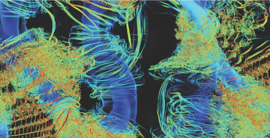
The large-domain Case 1 evolution is shown in Figure 2 from an early stage of KH billow formation (denoted 0 T_b) to a time 2.25 T_b later. The interval spans the dynamics that arise in small domains without T&K influences [18,19] and the T&K dynamics identified to date enabled by large domains noted above. An adaptive λ₂ color scale is employed separately at each time in order to reveal vortex features spanning a wide range of intensities. Specifically, the KH billow cores intensify significantly from 0 to 2.25 T_b, but appear to diminish due to the emergence of much more intense smaller-scale dynamics.

These fields reveal a diversity of T&K dynamics at larger and smaller scales, the larger of which are the major drivers of strong turbulence thereafter. All the KHI T&K dynamics emerge and drive strong turbulence transitions within 2.25 T_b, and largely prior to significant transitions by secondary CI and KHI. The T&K dynamics include:

(1)

initial links between mis-aligned emerging KH billow “ends” and continuous adjacent billows (sites “a”);

(2)

additional links of mis-aligned emerging KH billows where one billow “end” links to two billows (sites “b”);

(3)

large-scale vortex tubes emerging on the intensifying vortex sheets between KH billows where they exhibit significant phase variations along y that link adjacent billows as they intensify (sites “c”);

(4)

initial large-scale vortex knots driven by links between billow cores and/or large-scale vortex tubes (sites “d”);

(5)

smaller vortex tubes that form where adjacent billows exhibit weaker phase variations along y (sites “e”);

(6)

initiation of large-scale twist waves in the billow cores by the emerging knots (sites “f”) that propagate along the billow cores thereafter.

Secondary instabilities arising in the presence and/or absence of T&K dynamics by 1.5 T_b include the following:

(7)

secondary KHI on the intensifying vortex sheets that are enhanced where billow curvature increases stretching and intensification of the vortex sheets between adjacent KH billows (sites “g”);

(8)

initial secondary CI in the outer billows where they exhibit rapid intensification with and without apparent T&K enhancements; see sites “h” in the regions having the largest negative λ₂ (red) at 0.75 and 1.5 T_b;

(9)

a billow-pairing event, which can also occur in the absence of varying KH billow phases along y (site “i”).

Note that vortex tube “ends” and knots discussed here and below are sites where apparently distinct features appear to “attach”. However, vortex field lines are continuous and distinct features cannot attach; see the more detailed discussion of Case 3 below.

The Case 1 λ₂ fields at 1.5 and 2.25 T_b in Figure 2 reveal dramatic progressions from an initially laminar flow to emerging and/or intense turbulence arising from diverse KHI dynamics. All the T&K dynamics identified at 1.5 T_b except the billow-scale twist waves yield strong turbulence or its precursors revealed by intense, small-scale λ₂ features at 2.25 T_b. However, the occurrence and character of many features at small scales cannot be seen in Figure 2. Hence, expanded views of the λ₂ fields at smaller and larger y at 2.25 T_b are provided in Figure 3 and Figure 4 and in a subdomain spanning 1.6 L and 2.1 L along x and y, respectively, in Figure 5. These views reveal a diversity of transitional dynamics, several types of responses of which remain laminar in some regions and exhibit initial transitions to turbulence elsewhere. Note that the imaging was restricted to |z| < 0.2 L because of the very large data files. This enables viewing into the billow cores where upward displacements at their larger displacements toward positive x exclude secondary CI from the volume viewed. 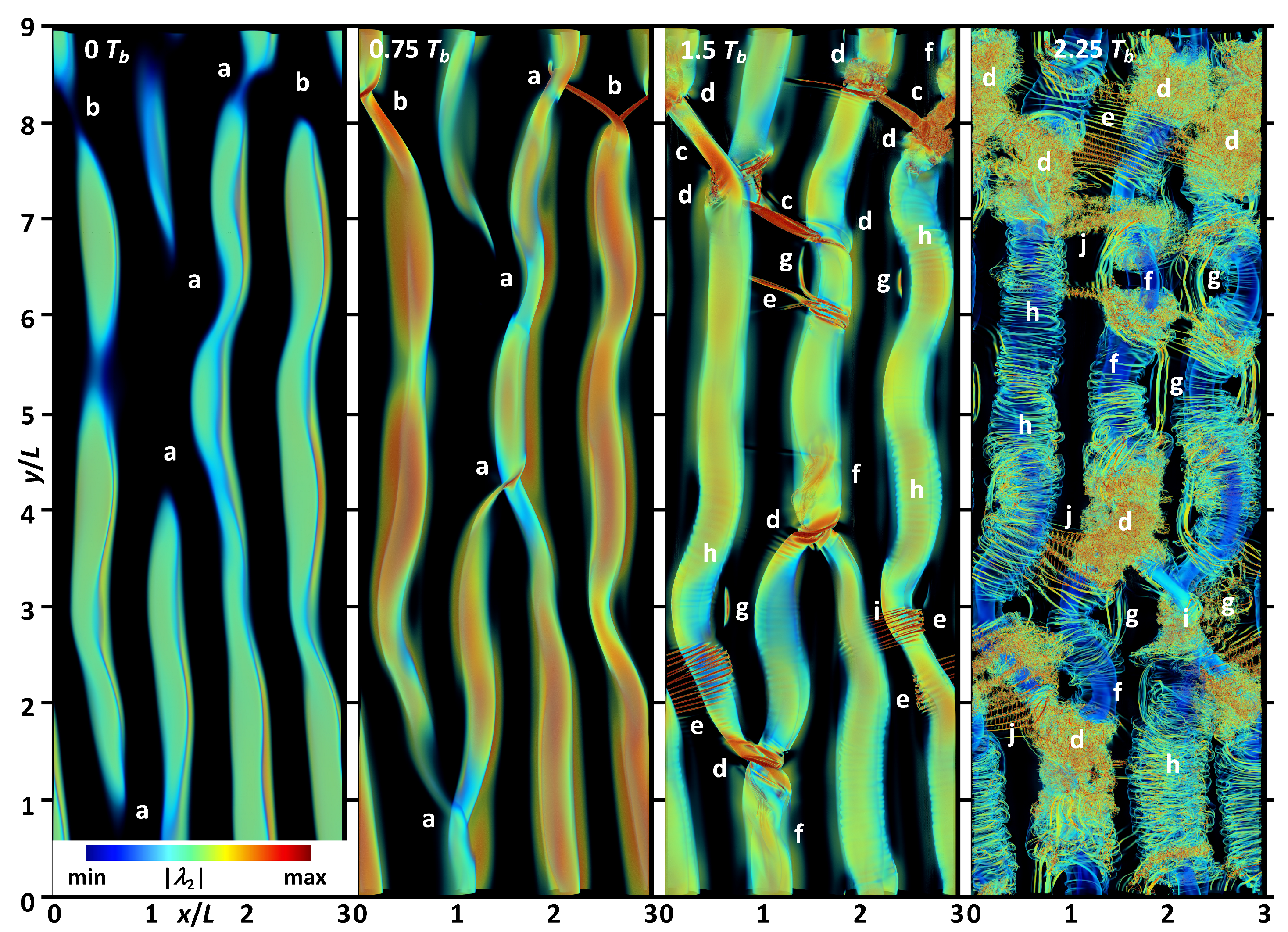Examples seen in Figure 3 and Figure 4, and the zoomed view in Figure 5, include the following:

(1)

small-scale vortex tubes between adjacent billows that remain laminar in some regions (sites “e”), but which exhibit links among them that emerge as secondary T&K dynamics on the vortex sheets, and become intense and initiate breakdown as they wrap over the KH billows at larger x (sites “j”);

(2)

secondary KHIs on the intermediate vortex sheets that are largely laminar, but exhibit mutual interactions driving smaller scale features in multiple regions (sites “g”);

(3)

secondary CIs at multiple sites that achieve large amplitudes and initiate mutual interactions driving emerging smaller-scale responses (sites “h”);

(4)

regions in which secondary KHIs and CIs evolve in increasing proximity where the vortex sheets wrap around the KH billows and initiate turbulence transitions among roughly orthogonal vortices (sites “k”);

(5)

increasing billow core displacements along x that are coherent along y with λ_y~2L (sites “l”) denoted a “crankshaft” instability, for which there is now significant observational evidence and are seen to arise in the final field in Figure 2 in the two KH billows at upper right;

(6)

emergence of these various dynamics in close proximity that also excite larger- and smaller-scale twist waves on the billow cores, vortex tubes, and smaller-scales vortices arising from larger-scale events (sites “f”).

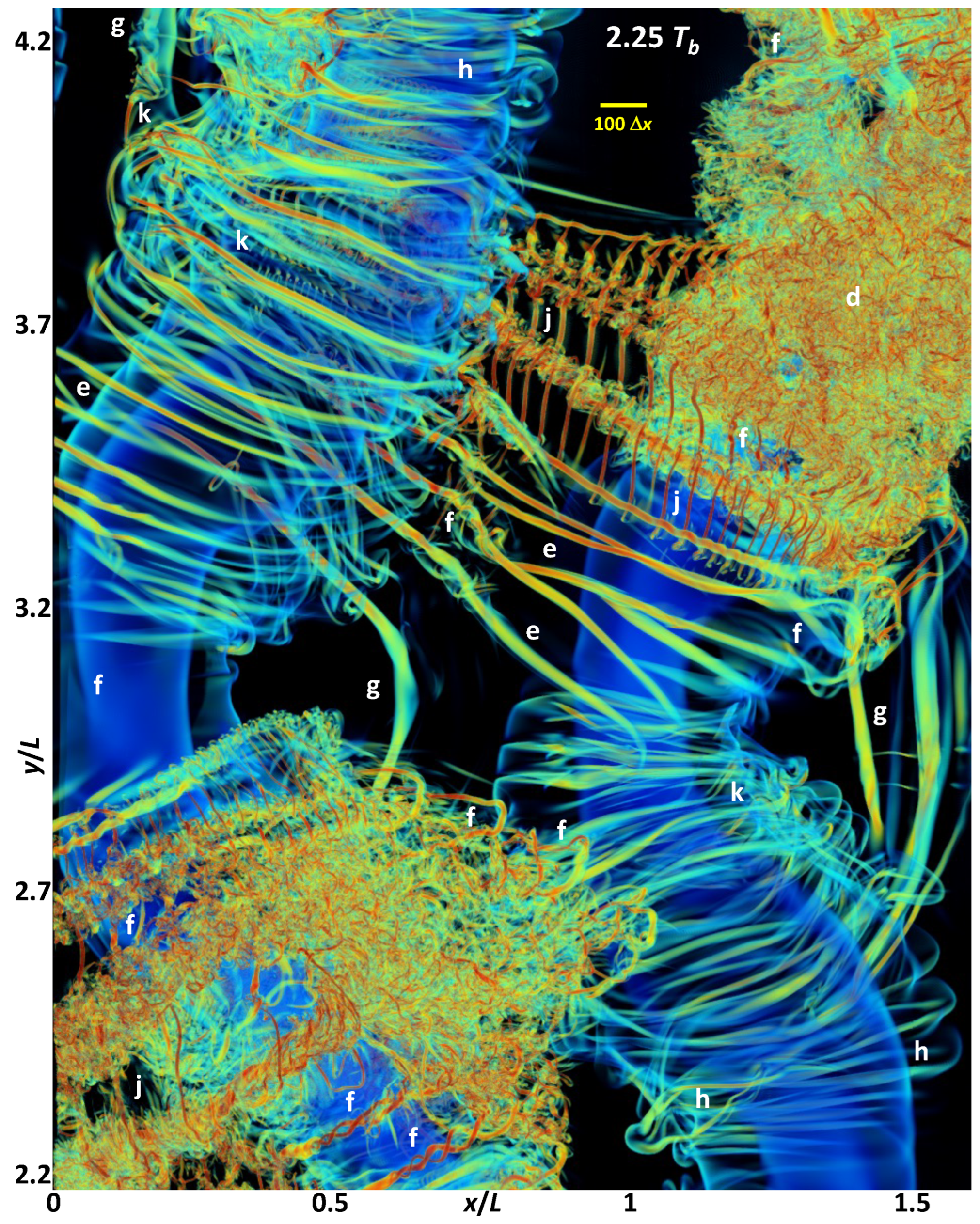
Figure 3. An expanded view of the 3-D imaging in Figure 2 at 2.25 T_b for y/L = 0–4.5. Feature labels are as in Figure 2. Note the yellow bar having a length of 200 ∆x for reference. The dashed yellow rectangle indicates the region shown with a zoomed view in Figure 5.

Figure 3. An expanded view of the 3-D imaging in Figure 2 at 2.25 T_b for y/L = 0–4.5. Feature labels are as in Figure 2. Note the yellow bar having a length of 200 ∆x for reference. The dashed yellow rectangle indicates the region shown with a zoomed view in Figure 5.

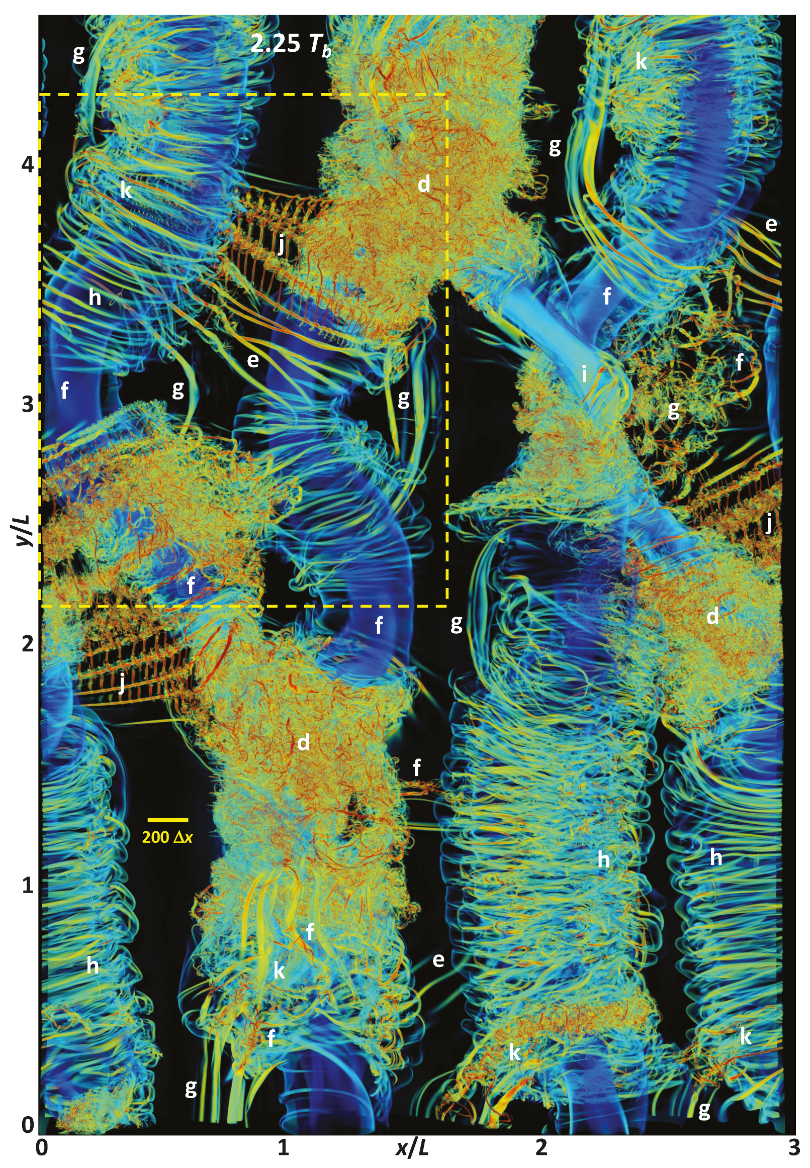
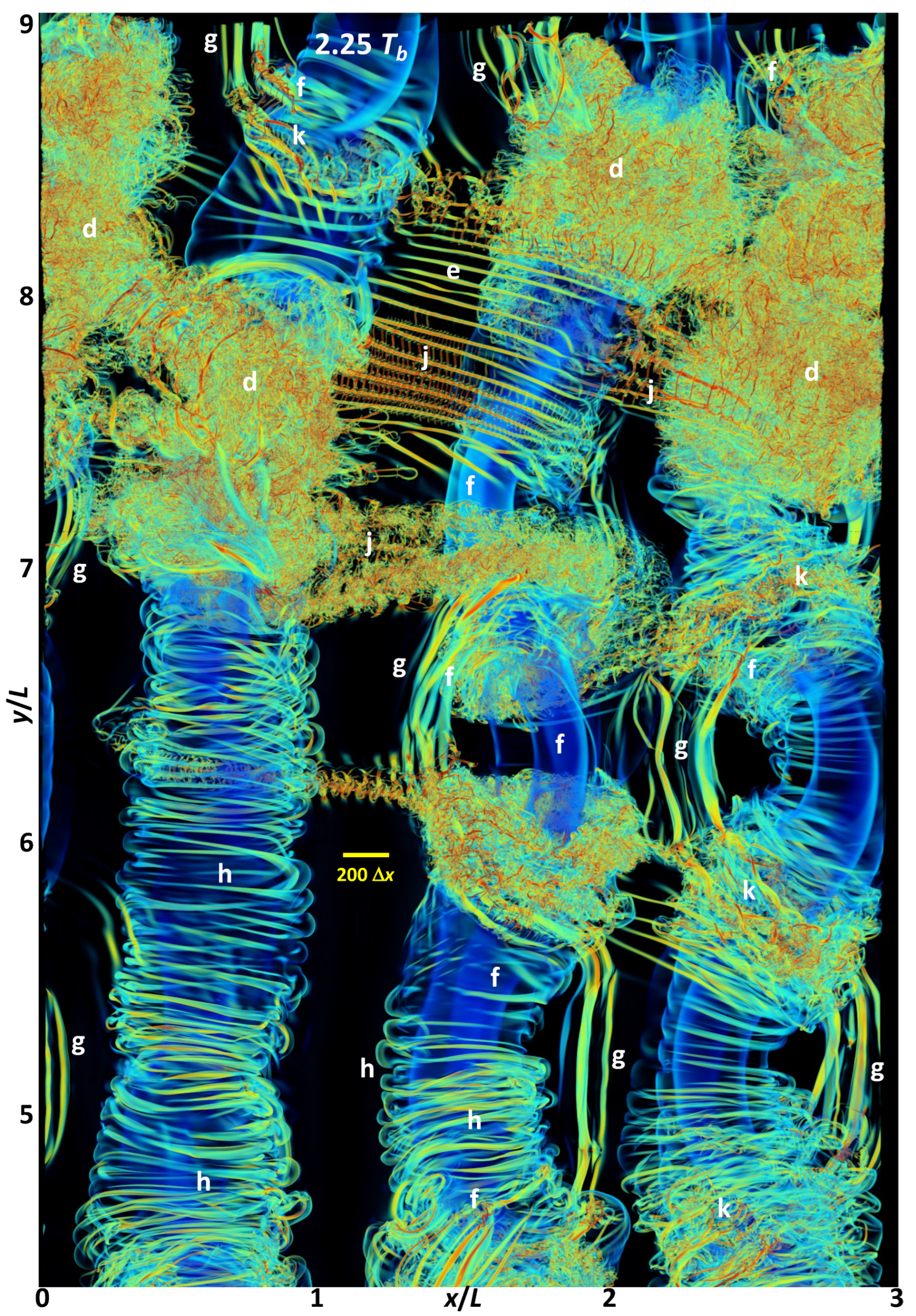
Figure 4. As in Figure 3, for the portion of the domain for y/L = 4.5–9. Note the 200 ∆x reference.

Figure 4. As in Figure 3, for the portion of the domain for y/L = 4.5–9. Note the 200 ∆x reference.

Figure 5. An expanded view of the yellow rectangle in Figure 3, showing smaller-scale features in greater detail. Feature labels are as in Figure 2, Figure 3 and Figure 4. Note the 100 ∆x reference at top.

Figure 5. An expanded view of the yellow rectangle in Figure 3, showing smaller-scale features in greater detail. Feature labels are as in Figure 2, Figure 3 and Figure 4. Note the 100 ∆x reference at top.

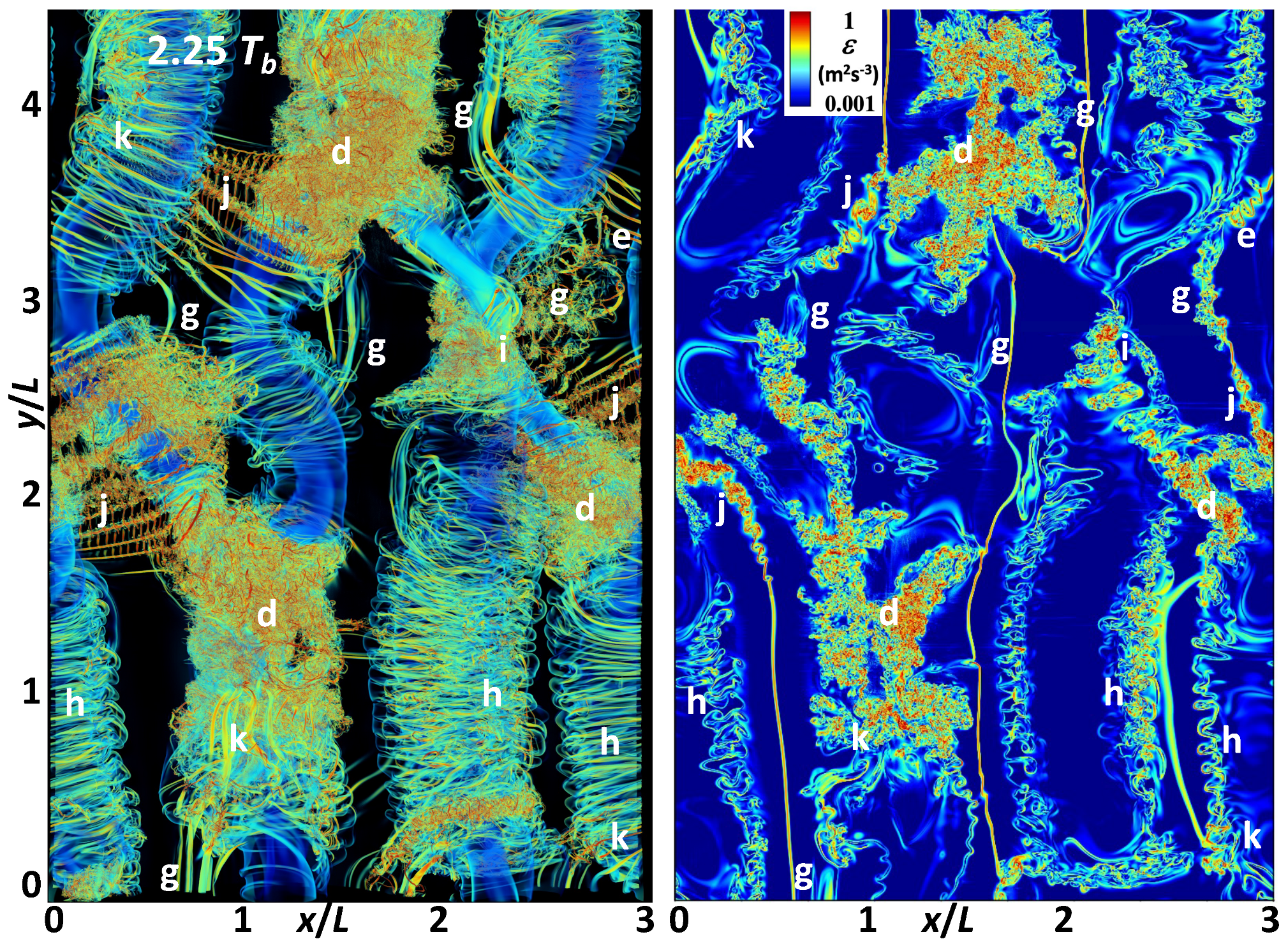
The importance of various T&K dynamics is assessed qualitatively using their contributions to local energy dissipation rates, ε. We employ ε(x,y) at z = 0 at 2.25 T_b for this purpose because volumetric views, as used for λ₂(x,y) in Figure 2, Figure 3, Figure 4 and Figure 5, mask the peak ε in deep T&K events such as knots by much weaker ε at the event extrema in z. Comparisons of λ₂ as shown in Figure 2, Figure 3, Figure 4 and Figure 5 and log₁₀ε(x,y) at z = 0 at 2.25 T_b are shown in Figure 6 and reveal the following sites to drive the strongest dynamics and ε arising by 2.25 T_b:

(1)

the intense initial knots (sites “d”) account for the largest ε spanning the largest regions horizontally;

(2)

smaller knot regions arising from the billow pairing (and merging) event (site “i”) achieve comparable peak ε, but are more confined spatially;

(3)

secondary KHI T&K events along the inclined vortex sheets (sites “j”) yield comparable peak ε because this is where the vortex sheets are most intensified by adjacent KH billows having large phase variations along y.

Figure 6. As in Figure 3 (left) and the corresponding log₁₀ε(x, y) at z = 0 and 2.25 T_b (right).

Figure 6. As in Figure 3 (left) and the corresponding log₁₀ε(x, y) at z = 0 and 2.25 T_b (right).

Additional sources of emerging instabilities and weaker, but increasing, ε in order of importance include the following:

(4)

regions in which secondary KHI are entrained over/under KH billows into close proximity to CIs induce their close interactions and turbulence transitions (sites “k”);

(5)

intensifying secondary KHIs where they are enhanced by distorted KH billows (site “g” at larger x than the billow pairing event);

(6)

intensifying and interacting CIs in the billow exteriors inducing initial turbulence transitions (sites “h”).

These various dynamics enable several broad conclusions:

(7)

large-scale KHI T&K dynamics drive turbulence events that are more intense than those occurring in their absence, consistent with the initial DNS cited above;

(8)

large-scale KHI T&K dynamics induce intensification of, and interactions among, smaller-scale secondary CIs and KHIs yielding localized, intense features at small scales without large-scale, energetic precursors;

(9)

secondary CIs and KHIs also exhibit smaller-scale, but much weaker, self-interactions without large-scale influences on comparable time scales.

4. Idealized Small-Domain KHI T&K Imaging

We now describe three small DNS of idealized KHI T&K interactions that reveal the transitions to turbulence seen in vorticity, described by λ₂, and helicity H. Case 2 is motivated by sites in the Case 1 DNS seen to drive the initial vortex knots (sites “b” to “d” in Figure 2, Figure 3, Figure 4, Figure 5 and Figure 6), where two KH billows link to one via strong vortex tubes. Case 3 approximates sites “e” in Case 1 in which two billows link via multiple, smaller vortex tubes where the billows exhibit common phase variations along their axes. Case 4 examines the mutual interactions of two orthogonal linear vortices in close proximity that approximate interactions seen to arise in previous large-eddy simulations (LES) and DNS of turbulence transitions due to KHI T&K [4,5] and similar dynamics in other turbulence transitions.

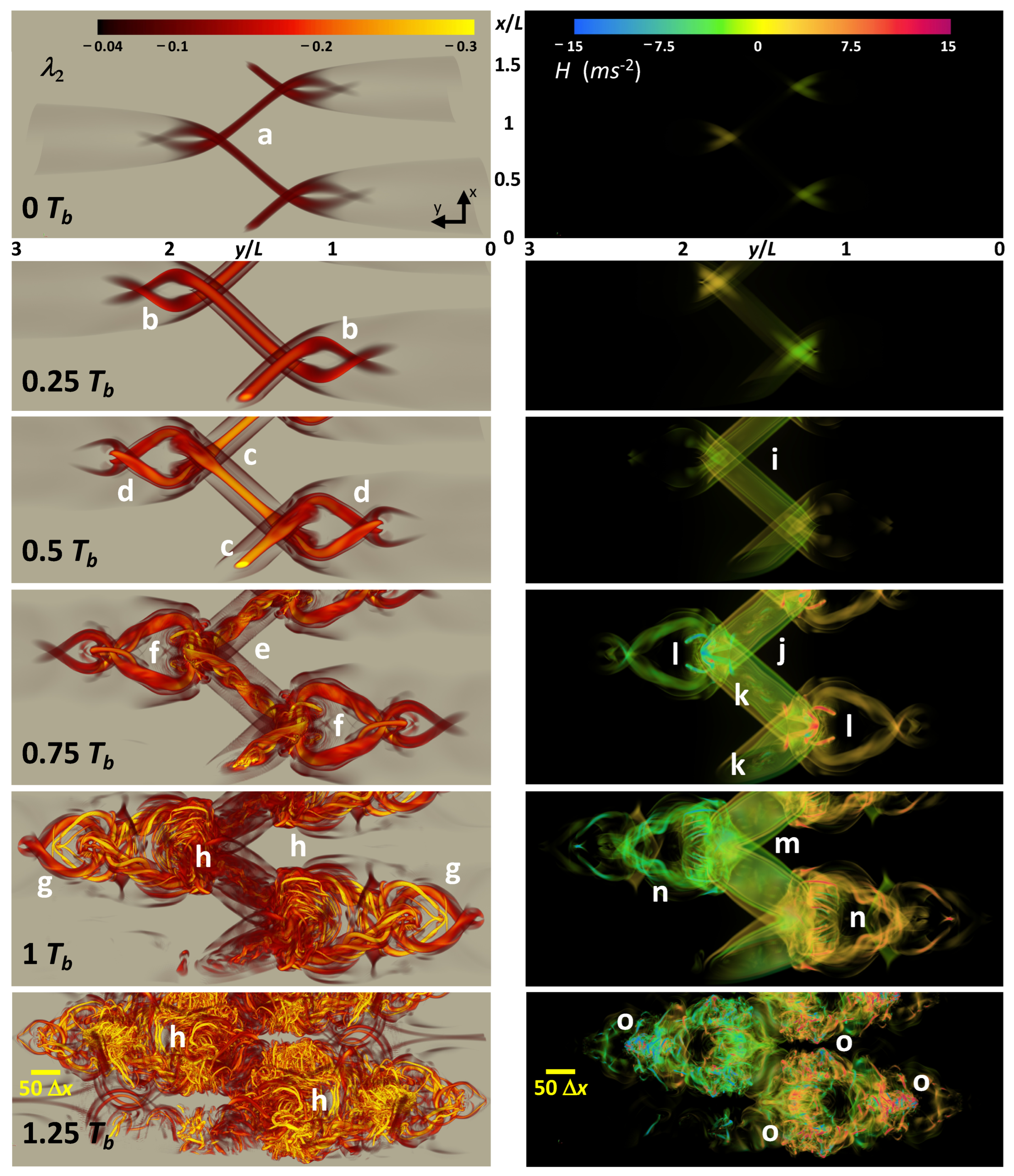
4.1. Case 2: One KH Billow Linking to Two Billows along Their Axes

Case 2 is an idealized version of the sites labeled “b” at 0.75 T_b in Figure 2. It was performed in a small periodic domain containing sites linking one KH billow to two, one of which is shown here. An initial Ri = 0.1 (Fr = 3.16) was employed as for Case 1, but a smaller Re = 2000 was specified to restrict the evolving dynamics to larger spatial scales. Three-dimensional imaging of λ₂ and H spanning 1.25 T_b is shown in Figure 7, viewed from above and negative x, with positive spanwise vorticity ζ_y to the left. Successive images are expanded to reveal the details as they intensify and cascade to smaller scales. Accompanying videos, Case2a.mp4 and Case2b.mp4 in the Supplementary Materials, provide animations of the of λ₂ and H evolutions shown at left and right in Figure 7.

The first images show a time at which weak initial vortex tubes induced by stretching of the intermediate vortex sheets have linked by wrapping over (under) the billow ends at larger (smaller) y (sites “a” in λ₂ at left) and induced initial mode-2 twist waves in the billow cores. These features and interactions intensify rapidly due to continuing KH billow roll-up and vortex sheet stretching, yielding strong initial mode-2 twist waves in the billow cores by 0.25 T_b (sites “b”) and differential vortex stretching and compression (sites “c”) where the tubes link to the billow cores by 0.5 T_b. These evolving dynamics act as strong sources of additional, smaller-scale, twist waves on the vortex tube “ends” and on the initial, larger-scale twist waves in the billow cores seen emerging at 0.5 T_b (sites “c” and “d”). They intensify dramatically and drive increasingly smaller twist waves that account for the initial turbulence transitions in the vortex tubes and their links to the billows by 0.75 T_b (sites “e” and “f”). The further evolution seen at 1 and 1.25 T_b reveals extensions of these dynamics along the billow cores (sites “g”) and to smaller scales and higher intensities in the turbulence inertial range within the emerging vortex knots (sites “h”).

The corresponding Case 2 evolution of helicity, H, is shown on the right in Figure 7 from the same perspective. H is also very weak during the initial links between mis-aligned KH billows because both ζ_y and the initial axial velocities, primarily u₂ = v, are very small. These features intensify by 0.25 T_b and exhibit positive (negative) H where the emerging tubes link to the KH billows, implying positive (negative) v at larger (smaller) y for ζ_y > 0. By 0.5 T_b, the vortex tubes have expanded and evolved oppositely signed H sheaths by entraining the vortex sheets from larger and smaller x and y (sites “i”) on which the tubes arose.

The vortex tubes expand significantly by 0.75 T_b and exhibit intensifying H sheaths at increasing radii (sites “j”) that remain laminar beyond 1 T_b. However, the most significant features arising by 0.75 T_b are strong H signatures of emerging smaller- and larger-scale twist waves on the vortex tubes and on the initial, larger-scale twist wave vortices extending into the billow cores (sites “k” and “l”, respectively). In both cases, these reveal finer-scale, more variable features than seen in λ₂ for the opacity scales employed here. The H fields thus enable probing of the interiors of the superposed twist waves in the vortex cores and the evolving vortex knots emerging by 0.75 T_b and intensifying thereafter. H is highly correlated with twist waves on the vortex tubes, as seen in the billow cores at 1 T_b, but its magnitude and sign are determined by the twist wave rotation and larger-scale velocity field along their axes.

Smaller-scale twist waves seen in H in the vortex tubes at 0.75 T_b are seen to break down to smaller, weaker vortex features by 1 T_b (sites “m”). Because these dynamics are largely confined to the vortex tube interiors, the vortex sheaths around the tubes remain intact. In contrast, the larger-scale twist waves in the billow cores emerging by 0.75 T_b exhibit rapid intensification by 1 T_b (sites “n”) and break down to very small-scale, but coherent, features by 1.25 T_b (sites “o”). As noted above, these responses also reveal that H imaging identifies smaller-scale, apparently more intense, vortex features in the centers of the vortex knots that are masked by vortex features having smaller H at larger radii.

Intensifying and expanding twist wave interactions in the vortex tubes drive the breakup of the initial H sheaths by 1.25 T_b. These interactions also drive the most intense H within the billow cores where they first arose: at sites “l” at 0.75 T_b, sites “n” at 1 T_b, and sites “o” at 1.25 T_b. Because H magnitudes depend on larger-scale advection, however, λ₂ is a more confident indicator of emerging turbulent vorticity dynamics.

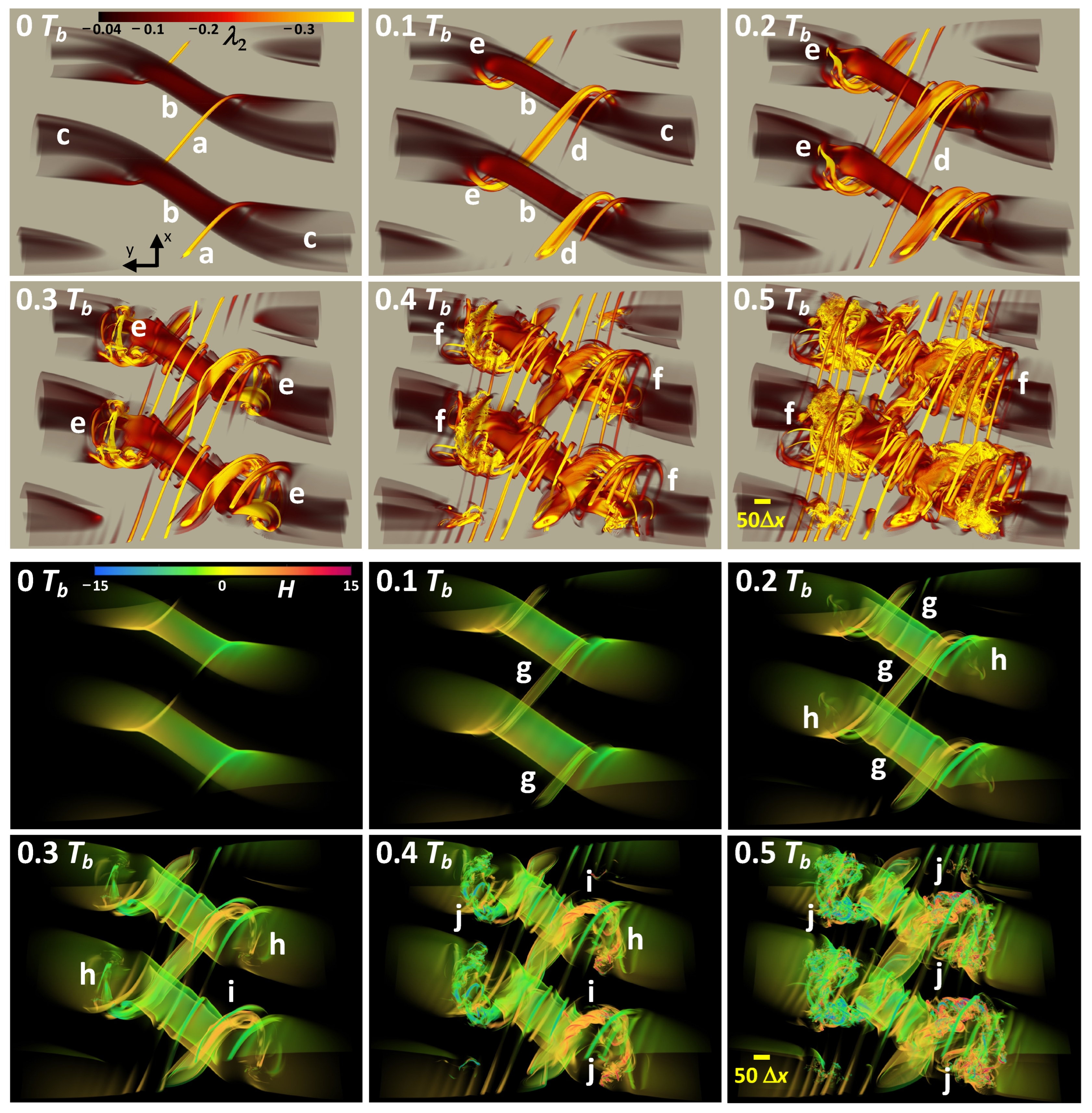
4.2. Case 3: Two KH Billows Having Varying Phases Linking via Smaller Vortex Tubes

Case 3 is an idealized version of the sites labeled “e” at 1.5 T_b in Figure 2. It was performed in the Case 2 domain to explore the λ₂ and H evolutions arising where adjacent billows exhibit common phase variations along their axes. Case 3 employed a smaller Ri = 0.05 (Fr = 4.47) to enable a more rapid evolution of small-scale vortices than in Case 1 and a smaller Re = 2500 to restrict the vorticity dynamics to larger spatial scales. Case 3 imaging of the λ₂ and H fields spanning 0.5 T_b is shown at top and bottom in Figure 8 in a subdomain spanning the region of varying billow phases viewed from above with positive x upward and positive y to the left. Accompanying videos, Case3a.mp4 and Case3b.mp4 in the Supplementary Materials, provide animations of the of λ₂ and H evolutions shown in Figure 8.

The λ₂ image at 0 T_b shows emerging vortex tubes (sites “a”) having positive ζ_y and negative ζ_x wrapping under (over) the KH billows at smaller (larger) x having positive ζ_y and ζ_x. The orthogonal alignments of these features, and their co-rotation, induce differential axial stretching and intensification, or compression and weakening, at different sites. The induced motions cause the KH billows to intensify (weaken) at sites “b” (“c”) and the vortex tubes between adjacent billows to increase and intensify (sites “d”) and “attach” to the outer KH billows by 0.3 T_b (sites “e”), but they remain largely laminar at this time. Increasing vortex tube intensities and proximity beginning by 0.3 T_b drive increasingly rapid and intense vortex knot formations thereafter (sites “f”). These are seen to (a) entrain the KH billow cores and vortex tubes, (b) exhibit rapid cascades to nests of intense twist waves and small-scale vortices, and (c) become largely turbulent by 0.5 T_b.

Our discussion of Case 1 noted that vortex tubes appear to attach to the outer “edges” of the respective KH billows, and these same dynamics are seen at higher resolution in Figure 8 at 0 T_b. This field reveals that the vortex tubes arise on the vortex sheets wrapping over and under adjacent KH billows, hence are distinct because vortex field lines remain continuous and arose at different locations in the initial, undisturbed, shear flow. Thus, they only appear to “connect” to the KH billow, and lead to increasingly entangled “knots” accompanying the cascade to smaller scales.

Imaging of H in the lower panels of Figure 8 reveals a number of features that are similar to those described in Case 2 above. These include H sheaths of opposite signs arising around both vortex tubes linking adjacent KH billows and the KH billows where they are intensified via axial stretching by the emerging vortex tubes at 0.1 and 0.2 T_b (sites “g”). Small-scale H features also emerge and intensify thereafter where the vortex knots arise at sites “e” in λ₂ imaging in the upper panels of Figure 8 (sites “h”). The H fields reveal the emergence of large-amplitude twist waves from 0.3 to 0.4 T_b, seen in the λ₂ fields but displayed more clearly in H at these times (sites “i”). Additionally, the H imaging reveals the scales and character of strong vortex dynamics within emerging knots that are masked by smaller-scale, but intense, vortex features having strong λ₂ responses at 0.4–0.5 T_b (sites “j”).

4.3. Case 4: Orthogonal Linear Vortices in Close Proximity

Case 4 was also performed in a small idealized periodic domain to enable the exploration of vortex dynamics among two orthogonal linear vortices having differing radii, denoted r₀ and r₁ = 1.5r₀, the same peak rotational velocities v₀ at these radii, a core separation of 5 r₀, and a Lamb–Oseen radial form [20,21] for the vortex with radius r₀ and circulation Γ₀ given by

v(r) = (Γ₀/2πr){1 − exp[−1.26(r/r₀)²]}

(10)

Case 4 was motivated by the sites labeled “k” at 2.25 T_b in Figure 3, Figure 4 and Figure 5 that reveal the emergence of roughly orthogonal vortices in close proximity. These dynamics are distinct from those described in Cases 2 and 3 because the vortices exhibit no initial links. The environment was specified to be adiabatic (N = 0) to exclude baroclinic vorticity generation. Different vortex radii were specified to illustrate more general responses of roughly orthogonal vortices driven into close proximity by larger-scale advection at larger scales in the turbulence inertial range. 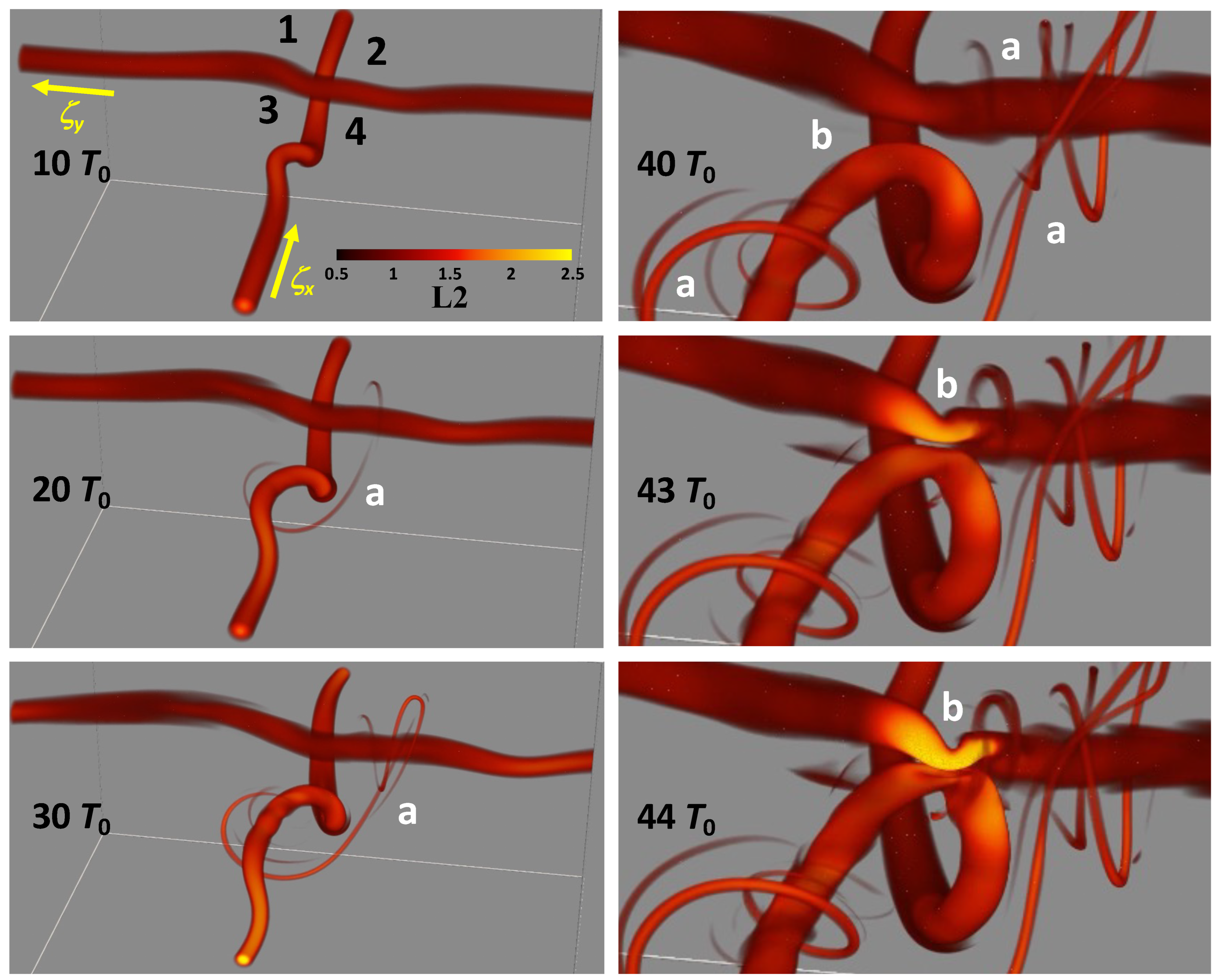As in Cases 2 and 3, a small Re = r₀v₀/ν = 2500 was specified to restrict the vorticity dynamics to resolvable spatial scales. Case 4 nevertheless yielded intense, small-scale vortex dynamics at late times. In order to show the evolution spanning very large λ₂ variations, we employed a color scale varying as √(−λ₂) denoted L2.

Imaging spanning 40 T₀ with T₀ = r₀/v₀ is shown with wider and zoomed subdomain views at earlier and later times in Figure 9 and Figure 10. Positive ζ_x and ζ_y for each initial vortex are shown with yellow arrows in the upper left panel of Figure 9. These imply converging (diverging) vertical motions in quadrants 1 (4) and downward (upward) motions in quadrants 2 (3). The dominant responses at early times are the distortions of the initial vortices driven by their mutual advection. Vortex distortions induce large-scale twist waves on each. Of these, the stronger distortions by the larger and stronger vortex impose much more dramatic responses on the weaker vortex along x. Induced perturbations to the larger vortex along y remain small until late times. Seen to emerge by 20 T₀ are small-scale vortices that are initiated in quadrant 4 (sites “a”). These arise due to the divergent motions along z and are distorted by, and advected around, the initial vortices. They intensify strongly, but play no roles in the transitions to turbulence in this event at the times shown in Figure 9. Accompanying videos, Case4a.mp4 and Case4b.mp4 in the Supplementary Materials, show the earlier and zoomed later evolutions displayed in Figure 9 and Figure 10.

Advection of the amplifying twist wave on the smaller vortex (with local ζ_x > 0) around the larger initial vortex (with primarily ζ_y > 0) drives these vortices into close proximity by 40 T₀ (site “b”), after which they begin to interact more strongly. The initial larger-scale vortex having ζ_y > 0 is intensified via stretching along y due to the strong curvature of the initial vortex having ζ_x > 0 in close proximity in this region. These vortex alignments drive increasingly strong interactions among adjacent vortex tubes having opposite local ζ_y. Surprisingly, it is the larger, weaker, vortex aligned initially along y that exhibits the most rapid intensification and kinking at this stage. Despite these apparently intense vortex interactions, there is no evidence of transitions to smaller-scale turbulence by 44 T₀.

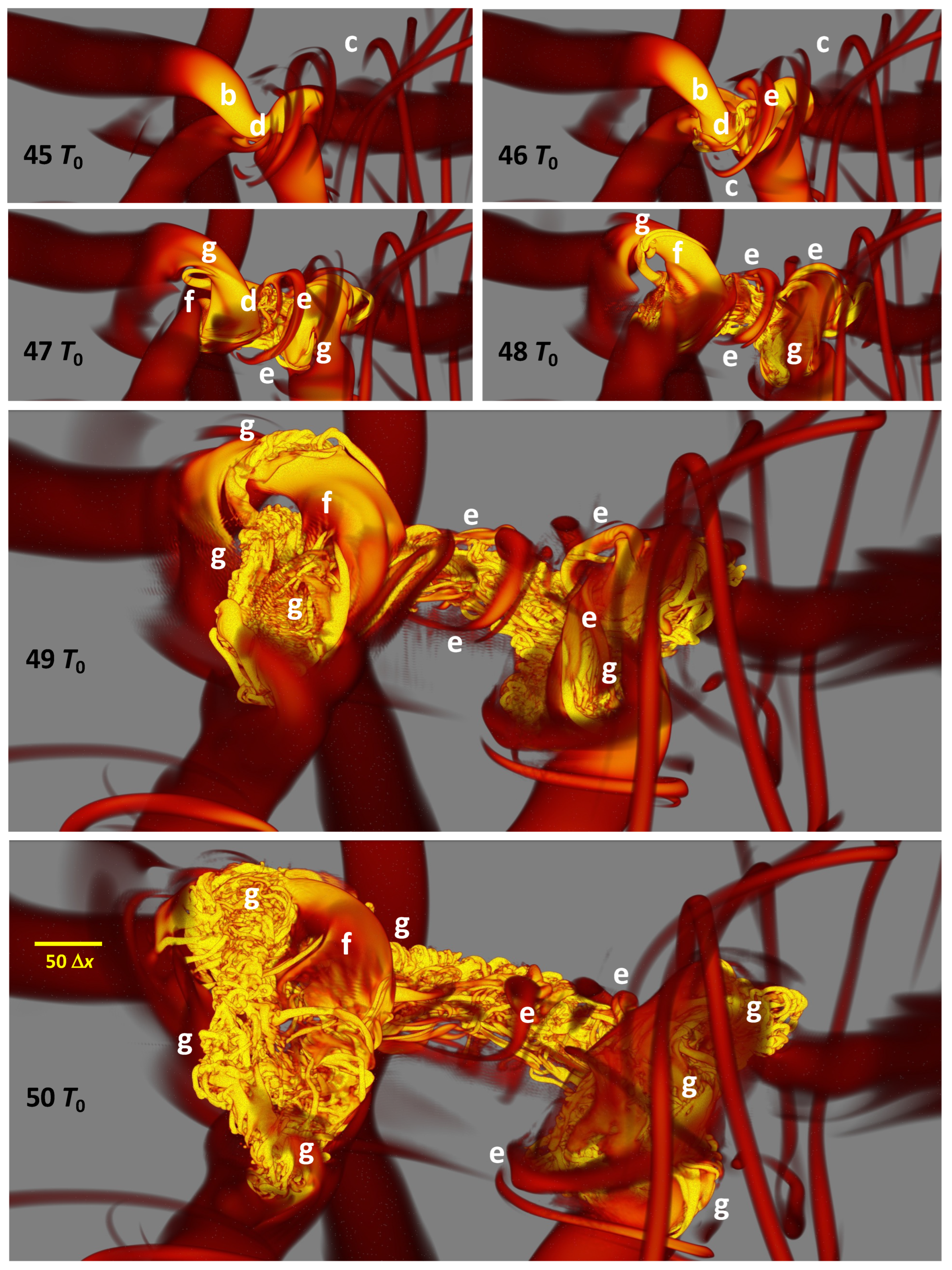
Turbulence transitions begin with emerging, small-scale, twist waves that arise and link initial vortices where they are most distorted at 45 T₀ (site “d”). These features intensify rapidly and exhibit smaller-scale twist waves that initiate the first turbulence transition by 47 T₀. Entrainment of smaller-scale vortices initiates additional sites driving initial turbulence transitions (sites “e”). However, the strongest transitions are driven by interactions among the intense, larger-scale, initial vortices. A small initial vortex “loop” (site “f”) arising by 47 T₀ expands by ~5 and 20 times by 48 and 49 T₀, respectively. These dynamics, and influences by the entraining smaller-scale vortices, drive the emergence of strong turbulence transitions at 47 T₀ (sites “g”) that expand throughout the large-scale vortex knot thereafter.

Importantly, the apparently most rapid and intense transitions are driven by direct interactions among the highly distorted initial vortices seen emerging by 47 T₀. While the larger-scale knot features are largely laminar to 47 T₀, smaller-scale vortices arising by 47 T₀ (sites “g”) intensify significantly by 48 T₀ and drive much stronger twist waves and more rapid turbulence transitions thereafter. See the Case4b.mp4 movie of this evolution.

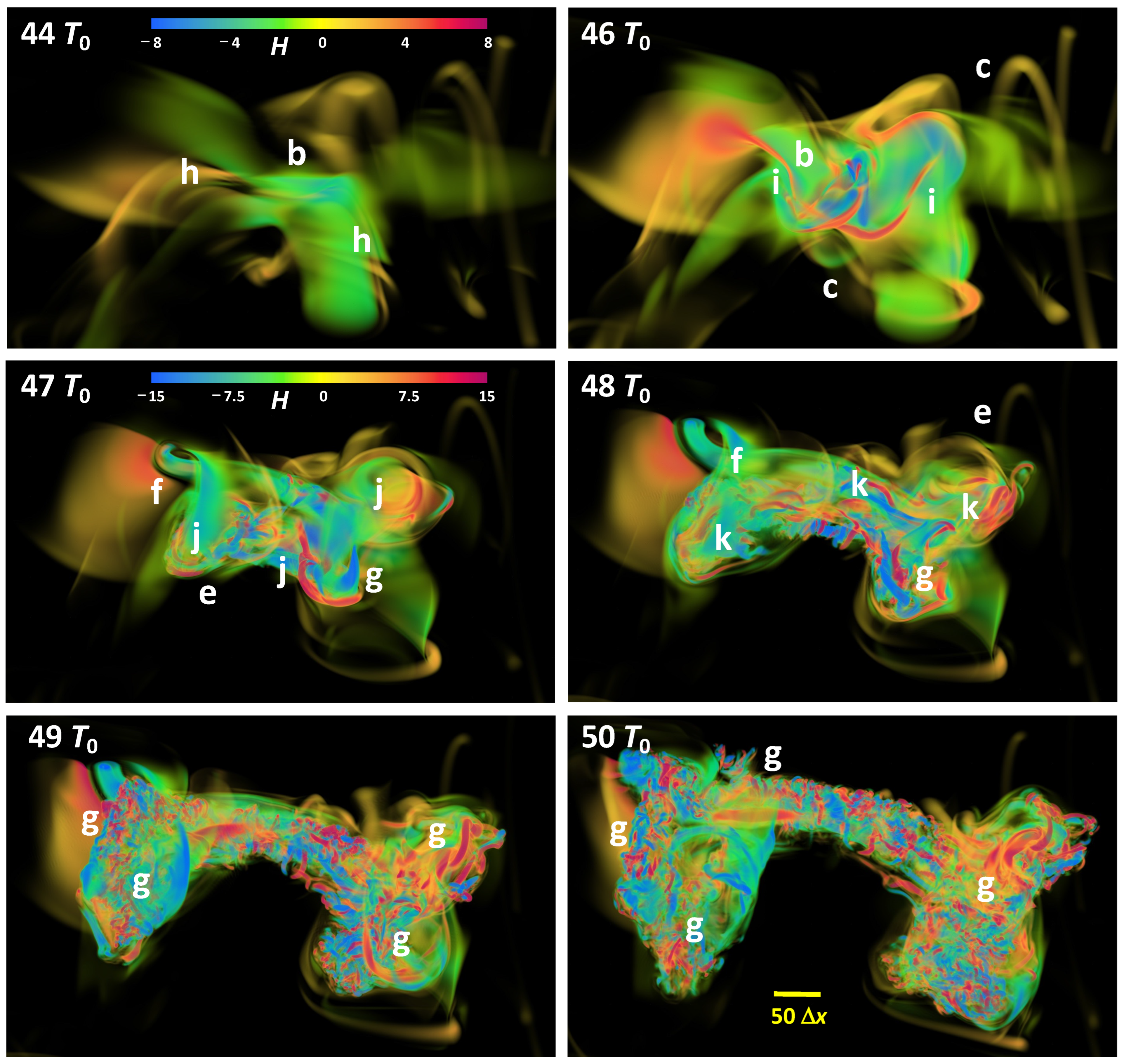
Case 4 H imaging corresponding to that for λ₂ shown in Figure 9 and Figure 10 from 44 to 50 T₀ is shown in Figure 11. Features seen in λ₂ imaging that exhibit similar responses in H are identified in Figure 11 with the same labels at the same times (sites “b”, “c”, “e”, “f”, and “g”). The λ₂ and H imaging at 44 T₀ reveal similar larger-scale features exhibiting weak H in the vortex cores, but also smaller-scale features including H sheaths and additional smaller-scale vortices that are not seen in the λ₂ imaging (sites “h”). The H imaging at 46 T₀ reveals the same vortex features at sites “b” and “c”, but also somewhat stronger and finer-scale features in the initial vortices that are not revealed by the λ₂ imaging (sites “i”). Similarly, the H imaging at 47 and 48 T₀ reveals several features noted in the λ₂ fields at these times in Figure 10 (sites “e”, “f”, and “g”), but the majority of significant features seen in H imaging highlight vortex structures occurring on much smaller scales that are not seen clearly in the λ₂ imaging (sites “j” and “k”, respectively). The final H imaging at 49 and 50 T₀ reveals the emergence of a diversity of features at multiple sites extending to very small spatial scales, some of which exhibit similar feature scales and orientations common to λ₂ imaging (sites “g”), but the majority of which do not.

5. Discussion

KHIs have been known for many years to drive turbulence and mixing in the atmosphere, oceans, and lakes. Their potential significance motivated a wide range of observational, laboratory, theoretical, and modeling studies exploring their evolutions, environmental responses, and secondary instabilities driving turbulence transitions for diverse Re, Ri, and Pr. Laboratory studies were the first to reveal KHI T&K dynamics clearly and recognize their significance [1,2,22], but they did not enable their quantitative analysis and interpretation. A wide range of theoretical and modeling studies of KHI spanning over 4 decades identified secondary KHIs and CIs occurring for idealized KHI in narrow domains that precluded T&K dynamics, e.g., [18,19] and references therein. However, it required new, high-resolution imaging of large-scale KHI at altitudes of ~80–90 km that resolved features and evolutions recognized as KHI T&K dynamics to guide initial modeling efforts [4,5].

KHI T&K dynamics now appear to be widespread throughout the atmosphere and likely oceans, lakes, and other stratified and sheared fluids [23]. They also arise readily in multi-scale GW environments [24], and may account for “missing” mixing inferred from global atmosphere modeling [25,26]. They likely also play similar roles in other geophysical and astrophysical environments [13], especially the oceans, where they may have implications for larger-scale stratification and overturning circulations [27,28], but their implications in these environments have yet to be explored.

The high-resolution modeling described here had two primary objectives. The first was to illustrate the more significant types of KHI T&K dynamics identified to date in observations and initial LES and DNS modeling. The second was to reveal specific T&K pathways to turbulence via imaging of feature evolutions in three idealized DNS designed to exclude competing T&K dynamics.

The first objective was addressed using a large, periodic DNS domain employing an initial noise seed that induced three or four initial KH billows at a finite amplitude along x at different y. This yielded (a) the expected secondary instabilities of idealized KHI, specifically secondary CI and KHI, (b) localized KH billow pairing, and (c) initial KHI T&K features driving turbulence transitions for the chosen initial conditions. These include the following in order of decreasing turbulence intensities:

(1)

intense vortex knots forming where KH billows are mis-aligned along their axes;

(2)

intense vortex knots forming where one or several larger-scale vortex tubes emerge on the intermediate vortex sheets and link adjacent billows where they exhibit larger phase variations along their axes;

(3)

delayed and weaker vortex knots that form where multiple, smaller-scale vortex tubes arise on the intermediate vortex sheets and link adjacent billows where they exhibit smaller phase variations along their axes;

(4)

secondary KHI T&K dynamics emerging on intensifying vortex sheets initiated by smaller-scale vortex tubes where billow phase variations are smaller;

(5)

a localized KH billow pairing event yielding a delayed and weaker knot;

(6)

regions where secondary KHIs are advected into close proximity to secondary CIs over and under the KH billows;

(7)

stretched and intensified secondary KHIs where billow curvature is large;

(8)

secondary CIs where KH billow phases are slowly varying along y.

The second objective was addressed by comparing imaging of (a) the rotational component of vorticity revealed by λ₂ as in our initial KHI T&K studies [4,5] and of (b) H employed previously to assess the degree of “knotted-ness” in turbulent flows [11,17]. In our applications, the λ₂ and H fields highlighted different features of the dynamics driving turbulence transitions. λ₂ imaging emphasized rapid transitions from larger-scale vortex interactions to smaller-scale turbulence where twist waves arose due to emerging strong, roughly orthogonal vortices in close proximity, specifically those initiating vortex knots in Case 1 and described in greater detail in Cases 2–4. These λ₂ fields captured the initial interactions and influences very well, including the emergence of twist waves at larger and smaller scales. As these dynamics progressed, however, smaller-scale vortex dynamics without significant H appear to have masked the larger-scale dynamics driving the emerging turbulence transitions in the vortex knot interiors in some cases.

The H imaging in Cases 2–4 revealed additional flow features that augmented our understanding of the emerging vortex character and the evolving dynamics prior to strong turbulence transitions. Importantly, it also revealed more persistent and coherent features at larger scales in the emerging vortex knot interiors extending to later times that were not revealed in the λ₂ imaging, but must continue to drive additional turbulence transitions extending to later times.

Kelvin vortex waves, or “twist waves” in our terminology, have received significant theoretical attention, e.g., [29], among many others. Multiple studies have revealed a broad spectrum of axial, azimuthal, and radial variations of vorticity and phase, and helical forms arising in varying environments. However, these methodologies cannot address the nonlinear dynamics of interacting vortices driving the turbulence cascade.

Our KHI T&K modeling addressed the vorticity dynamics of evolving multi-scale KHI environments driving the transitions to turbulence at Re = 5000 that is sufficient to enable a significant turbulence inertial range and more than 3 decades of scales resolved along the shear flow in Case 1. It was performed in a large domain enabling multiple KH billows and all of the transitional dynamics revealed in laboratory and theoretical studies, and atmospheric and oceanic imaging and profiling of KHI to date [23]. These dynamics rapidly become highly nonlinear and increasingly complex due to vortex interactions that are not possible to address via other methods. Where emerging KH billows exhibit mis-aligned or varying phases along their axes, they induce additional vortex stretching of the intermediate vortex sheets. These sites yield emerging, smaller-scale, vortex tubes evolving increasingly orthogonal alignments relative to the billow cores as they advect over and under adjacent billows. They appear to connect to the intensifying billow cores and exhibit rapidly intensifying mutual interactions thereafter. These “connections” are only apparent, however, because the interacting KH billow and vortex sheet vortices have their origins in very different regions of the initial shear flow.

The resulting interactions yield increasingly intense, smaller-scale vortices arising on each initial vortex that exhibit helical responses, most typically mode-1 single helix and mode-2 double helix twist waves. These arise due to axial and/or radial deformations or displacements that stretch, compress, strengthen, and/or weaken the initial vortices. Mode-1 twist waves propagate along the initial vortex typically without contributing to its breakup. Mode-2 twist waves, in contrast, “un-wrap” and fragment the initial vortex, driving the cascade of vorticity to smaller scales. Mode-3 and higher twist waves likely also arise, but are challenging to identify among the accelerating, intensifying, and tightly packed dynamics driving the emergence of vortex knots at the initial interaction sites.

Twist wave dynamics arise at successively smaller scales as orthogonal vortex alignments continue to emerge due to larger-scale advection accompanying the continuing KH billow evolutions. Their wavelengths along their parent vortices extend from ~2 L in the billow cores emerging prior to initial turbulence transitions seen at 0.75 T_b in Figure 2 to ~0.01 L in the vortex knots and secondary T&K dynamics at 2.25 T_b in Figure 5. They are also seen having wavelengths as small as ~10 ∆x at 50 T_b in Figure 10. Hence, twist waves play central roles in the cascade to smaller scales throughout the turbulence inertial range.

6. Summary and Conclusions

Results presented above reveal the various pathways to enhanced turbulence accompanying KHI T&K dynamics that arise where adjacent KH billows interact due to initial variations or mis-alignments along their axes. They are demonstrably widespread, and perhaps ubiquitous, in the atmosphere [23,24,30,31,32,33].

Current parameterizations attribute these responses to breaking GWs accompanying their amplitude growth with increasing altitude. However, more recent observations and DNS modeling suggest that KHI, and especially the expectation of enhanced responses due to their ubiquitous T&K dynamics, may contribute comparable or larger responses. Extensive aircraft measurements of turbulence in the lower stratosphere [34] in a strong mountain wave environment over and around the Drake Passage suggest that KHI, rather than GW breaking, appeared to account for the major turbulence at flight altitudes. A similar conclusion arose from a recent multi-scale GW DNS [24], where turbulence due to KHI was stronger than turbulence associated with GW breaking at later, potentially more realistic, stages of the simulation. Additionally, KHI arise at the most strongly stratified layers in a variable environment, thus potentially contribute more significant mixing. GW breaking, in contrast, arises in the least stable phases of the superposed GW field, hence yields mixing, in part at least, of an already weakly-stratified environment.

Mixing dynamics have been a significant interest of various communities for many years [35,36], and KHI T&K dynamics appear likely to play an important role in accounting for their influences and enabling improved parameterizations and applications.