1. Introduction
Water vapor is a critical component of the atmosphere, influencing weather, climate variability, and extreme weather events [
1]. Factors such as the coastal land position and topography influence the variations in water vapor, thereby causing regional differences in precipitation [
2,
3]. In the early stages, technologies like radio radiosonde stations, conventional balloon-borne soundings, and satellite-based microwave radiometers were used to measure the atmospheric water vapor content. While these methods were effective in detecting the water vapor content, they incurred high costs and exhibited lower quality [
1]. Over the past 20 years, with the advancement of GNSS technology and its integration with meteorology, GNSS has become a cost-effective, real-time, and low-error method for monitoring changes in atmospheric water vapor. In comparison with traditional methods of water vapor monitoring, GNSS technology offers several advantages [
4]. Consequently, GNSS atmospheric water vapor monitoring has been widely adopted, providing the field of meteorological research with higher precision, vast datasets, and real-time atmospheric water vapor information [
1].
In the process of deriving the PWV from GNSS-measured data, the conversion parameter K is used to transform the ZWD into atmospheric water vapor [
5]. The water vapor conversion parameter K is primarily influenced by the atmospheric weighted mean temperature Tm [
6]. Tm data can be obtained through mathematical calculations based on radiosonde data or layered meteorological data, but due to factors such as time and space, this method is not convenient for obtaining accurate Tm values. Therefore, scholars, both domestically and internationally, have conducted a series of studies and established Tm models suitable for different regions to provide convenience to users. Bevis and his team discovered a strong linear relationship between the Tm and Ts through their research on radiosonde data in North America and proposed the Bevis model [
7]. Böhm et al. introduced global troposphere models with different resolutions, namely, 1° × 1° (GPT2w-1) and 5° × 5° (GPT2w-5) [
8]. Zofia Baldysz and colleagues, using data from 109 radiosonde stations in Europe, derived a Tm model suitable for the European region through linear regression [
9]. Many researchers, including Huang, Mo, and Yao, established Tm regression models involving single and multiple elements [
10,
11,
12]. Scholars like Li Li and Li Jingwei used multiple linear regression to fit regional prediction models for the Tm in areas such as Hunan [
13], Xinjiang [
14], and Guangxi [
15] based on real-time radiosonde monitoring data. Li Jianguo and his team built a more applicable Tm model for the eastern part of China based on radiosonde and satellite measurement data [
16]. Mo Zhixiang, Li Xing, Li Jiahao, and others, while exploring the correlation between the Tm and Ts, incorporated various meteorological factors and seasonal variations, such as altitude and latitude. They developed high-precision Tm models for regions such as western China [
4] and the Qinghai–Tibet Plateau [
1]. Due to the vast expanse of inland areas, complex highland terrain, wide latitude coverage, and diverse climate types, it is necessary to construct Tm models based on the characteristics of each region’s topography.
This study investigated the relationship between the Tm, Ts, ln(e), and elevation H in the Qinghai–Tibet Plateau region using radiosonde data from 2008 to 2017. A weighted average temperature refinement model (XTm model) suitable for this region was developed based on the Bevis model by considering various factors, such as surface temperature, water vapor pressure, elevation, and annual and semi-annual periodic changes. The quality of the model was verified using radiosonde data from 2018 to 2019, providing a crucial reference for high-precision GNSS water vapor inversion and its applications in the Qinghai–Tibet Plateau region.
2. Materials and Methods
2.1. Study Area and Data Source
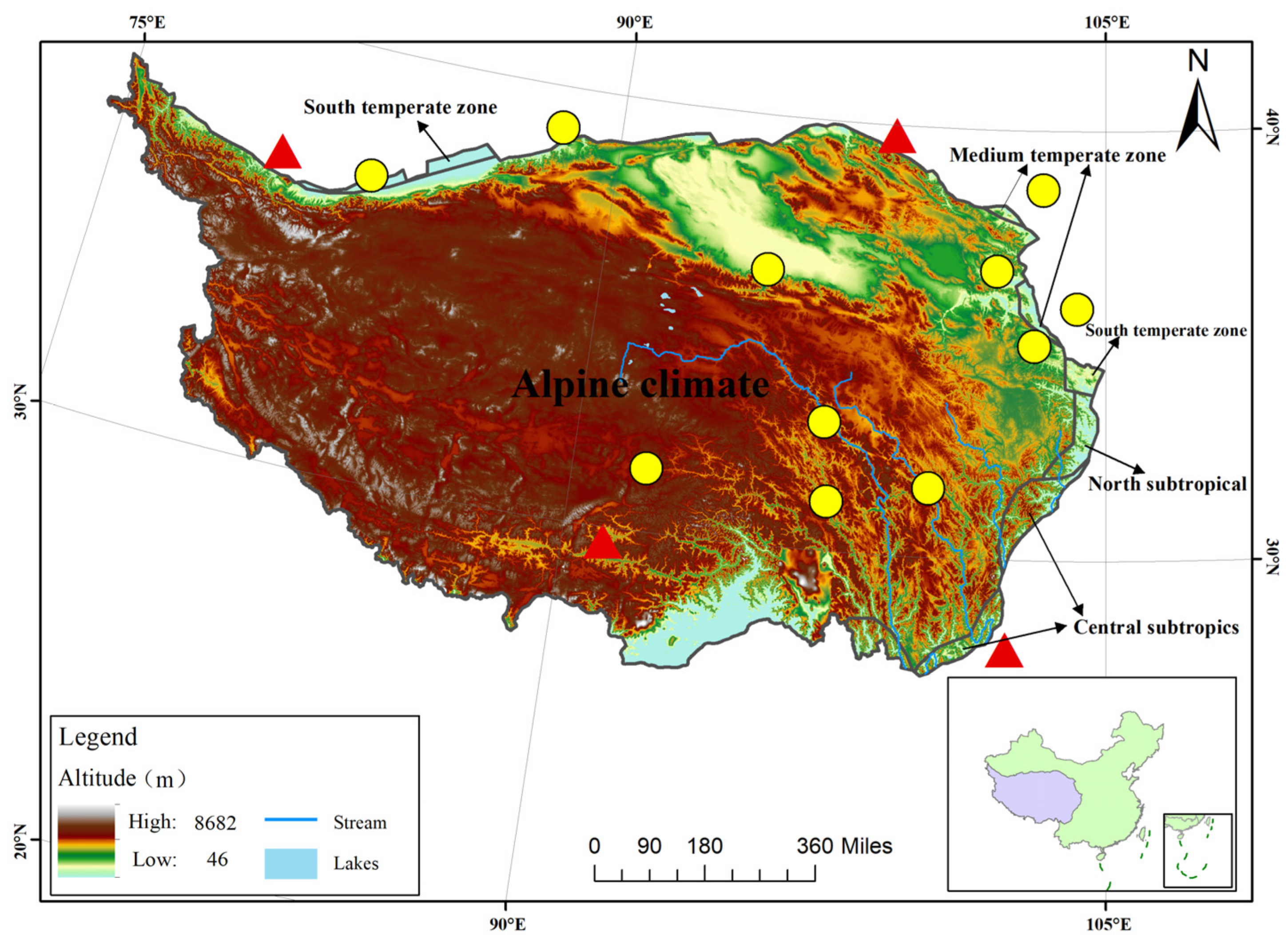
The Qinghai–Tibet Plateau is often referred to as the “Roof of the World”. It is located between 26°00′ to 39°47′ N and 73°19′ to 104°47′ E, covering the entire Tibet Autonomous Region and parts of Qinghai, Xinjiang, Gansu, Sichuan, and Yunnan provinces in China. The climate in the Qinghai–Tibet Plateau region is diverse and complex, with variations in the distribution of moisture at different altitudes. The intricate topography of the plateau itself contributes to its unique climatic characteristics. As the highest plateau on Earth, the Qinghai–Tibet Plateau’s high elevation can block, separate, and disrupt large-scale atmospheric circulation between the land and oceans in surrounding regions. This, in turn, affects the climate and precipitation patterns in neighboring areas and can even lead to extreme weather events and disasters. In the context of climate change in China and parts of the Northern Hemisphere, the Qinghai–Tibet Plateau plays a regulating, promoting, and feedback role.
The observational data were obtained from 17 radiosonde stations in the Qinghai–Tibet Plateau region from 2008 to 2019. These radiosonde data can be freely downloaded from the following website:
http://weather.uwyo.edu/upperair/sounding.html, accessed on 26 November 2023. The sounding station data primarily consist of the station’s geopotential height, latitude, and longitude, as well as daily surface observations of temperature (Ts), weighted mean temperature (Tm), atmospheric pressure (P
0), and water vapor pressure (e) obtained at 00:00 and 12:00 UTC each day.
This study selected observation data from 13 radiosonde stations evenly distributed in the Qinghai–Tibet Plateau region from 2008 to 2017 for the model construction and evaluates the quality of the established model using data from 17 radiosonde stations (including 13 modeling stations and 4 non-modeling stations) from 2018 to 2019. The distribution of radiosonde stations and relevant information from each station are shown in
Figure 1 and
Appendix A.
2.2. Data Processing
According to references [
17,
18,
19], the formula for deriving atmospheric water vapor content from GNSS is
. ZWD represents the zenith wet delay; PWV is the precipitable water vapor; and Π is the water vapor conversion coefficient, which is calculated using the following formula:
In Formula (1), , , , and .
When calculating the reference value for the Tm, it is obtained using a numerical integration method based on the water vapor pressure (e) and absolute temperature (T) at the corresponding levels of the radiosonde station integrated toward the top of the atmosphere. The formula is as follows:
In Equation (2) above, e represents the water vapor pressure, measured in hPa (hectopascals); T represents the atmospheric temperature, measured in K (Kelvin); h represents the vertical geopotential height above the station, measured in meters (m). The integration spans from the starting point at the radiosonde station all the way up to the top of the atmosphere. Conventional sounding data typically provide the relative humidity (RH) and absolute temperature (T), while water vapor pressure (e) cannot be directly obtained from the sounding data. According to reference [
18], the water vapor pressure can be calculated using the formula for dew point temperature (T
d) in relation to the saturation vapor pressure (e
s) when T is in Kelvin (T = T
d + 273.15). The formula used here is as follows:
In the process of evaluating the quality of the constructed weighted mean temperature models, it is necessary to calculate the root mean square (RMS) and bias for each model to reflect their quality. The formulas for the bias and RMS are as follows:
In Equations (5) and (6), represents the weighted mean temperature predicted by each model, represents the reference value of the Tm, and N represents the number of observed data points.
2.3. Tm from the Bevis Model
Although the quality of the Tm obtained from observations at sounding stations is high, the distribution of radiosonde stations is sparse, resulting in limited applications.
A commonly used empirical method is the Bevis model, which estimates the T
m based on the Ts observations. Bevis believed that there is a good linear correlation between the Tm and Ts. Therefore, Bevis used measured data from 13 radiosonde stations in the United States to obtain a linear observation equation (also known as the Bevis empirical formula) using the least squares method. Therefore, the Bevis model has been widely used worldwide due to its simple and practical characteristics.
2.4. Tm from the GPT2w Model
Bohm et al. [
8] added two parameters of the water vapor pressure vertical gradient and atmospheric weighted average temperature into the GPT2 model to obtain the GPT2w model, which further improved the quality of the GPT2w model. The GPT2w model can provide Tm values with resolutions of 1° × 1° and 5° × 5°. The Tm of the GPT2w model is calculated using Equation (8):
In Equation (8), DOY stands for the day of the year and the coefficients A0, A1, A2, B1, and B2 are determined based on a regular grid of 1° × 1° and 5° × 5°, namely, the GPT2w-1 and GPT2w-5 models, respectively. In this study, we chose the GPT2w-1 and GPT2w-5 models to use in the validation.
2.5. Correlation Analysis of Different Meteorological Factors with Weighted Mean Temperature
According to the available data, for the Qinghai–Tibet Plateau region, the existing models show significant differences between the fitted values of the weighted mean temperature and the reference values obtained through numerical integration. In this study, a correlation analysis of relevant variables affecting the weighted mean temperature was conducted. Variables that exhibited a strong correlation with weighted mean temperature in this region were selected, and a new Tm model was established based on their correlation characteristics. The following sections mainly discuss the correlation between the Ts; natural logarithm of water vapor pressure, i.e., ln(e); and H with the weighted mean temperature.
In this study, satellite measurements from 13 selected radiosonde stations within the Qinghai–Tibet Plateau region from 2008 to 2017 were used to analyze the correlation between different meteorological factors and weighted mean temperature.
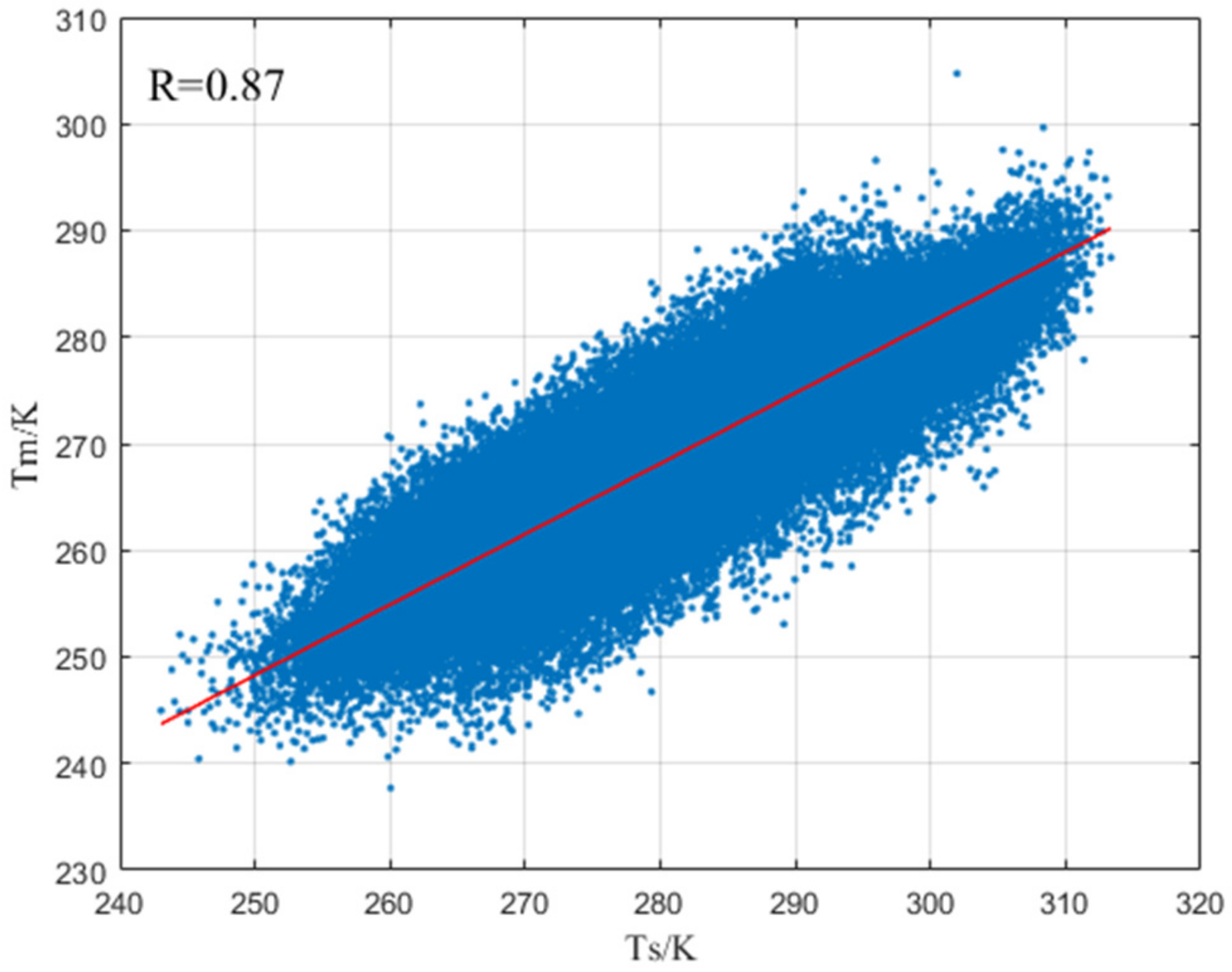
Figure 2 shows a schematic representation of the linear correlation between the Ts and Tm. It can be observed from the figure that the Ts and Tm in the Qinghai–Tibet Plateau region were positively correlated, indicating a strong correlation with a correlation coefficient of 0.87.
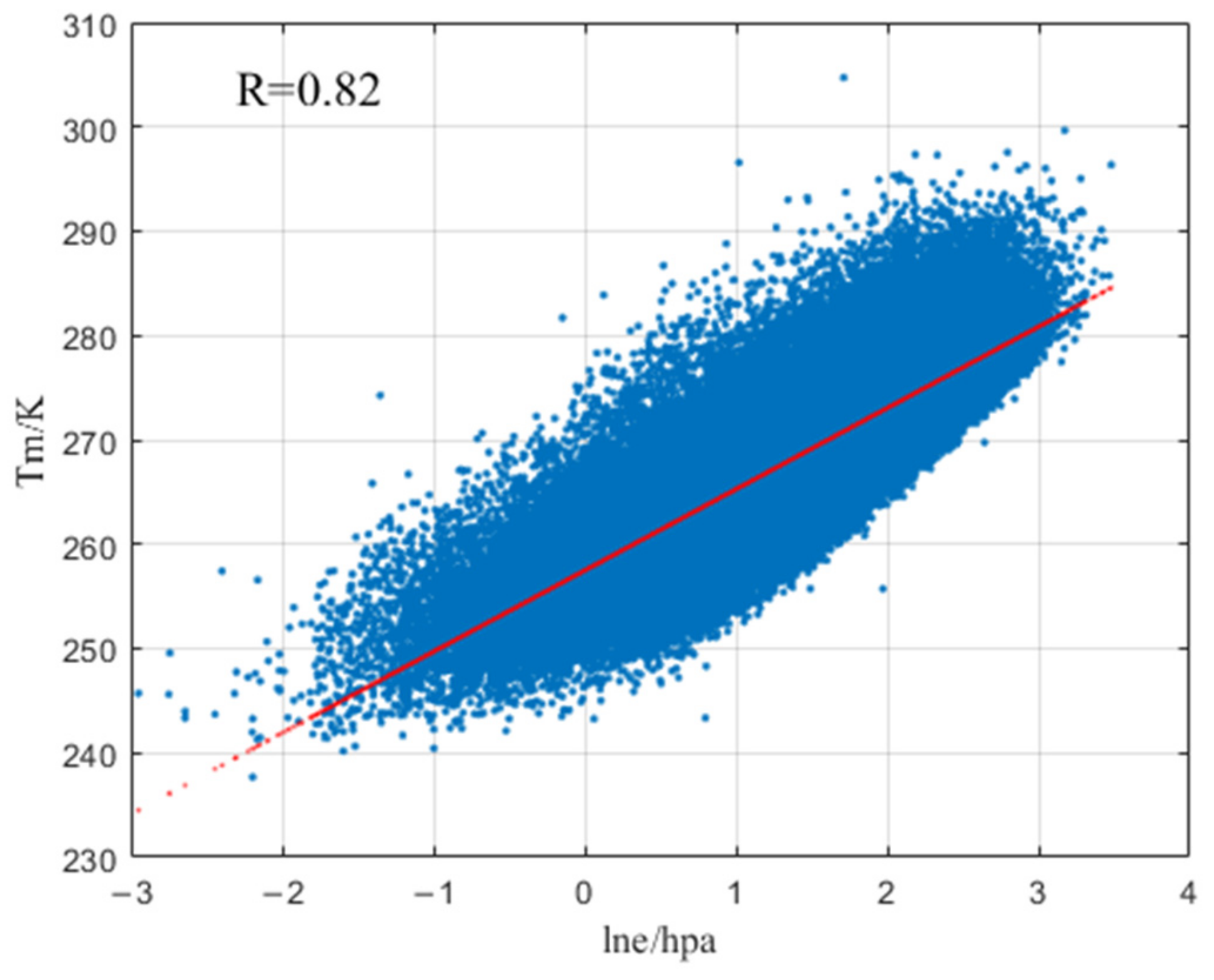
Figure 3 depicts the linear correlation between the ln(e) and Tm. From
Figure 3, it can be seen that the ln(e) in the Qinghai–Tibet Plateau region exhibited a good linear correlation with the Tm, with a correlation coefficient of 0.82.
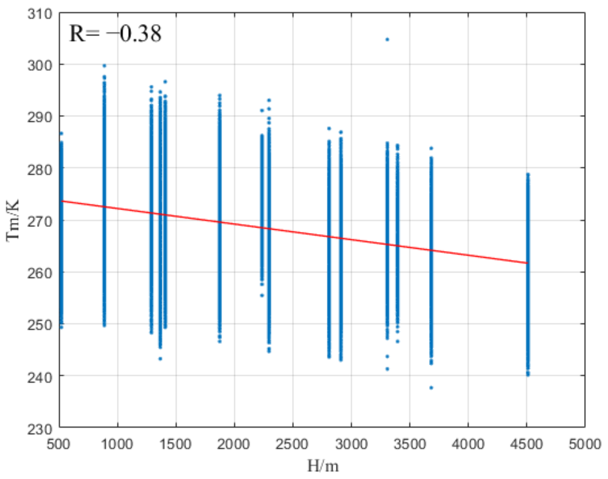
Figure 4 illustrates the linear correlation between the H and average Tm in the Qinghai–Tibet Plateau region. It explores the linear correlation between the Tm and H.
Figure 4 demonstrates that the H and Tm exhibited a strong negative linear correlation with a correlation coefficient of −0.38 in the Qinghai–Tibet Plateau region.
2.6. Construction of the Weighted Mean Temperature Model in the Qinghai–Tibet Plateau Region
Based on the analysis in the previous text, it was observed that the weighted mean temperature was strongly correlated with the Ts, ln(e), and H in the Qinghai–Tibet Plateau region. In addition to these spatial factors, the weighted mean temperature also exhibited annual and semi-annual variations with the passage of time [
17]. Although fitting empirical models can help to mitigate some errors, there are still residual periodic systematic errors, and the residuals of the Tm and Ts models remain noticeable [
20]. Therefore, to enhance the quality, the residuals were compensated for using trigonometric functions with annual and semi-annual frequencies. As a result, the atmospheric weighted mean temperature model in the Qinghai–Tibet Plateau region can be expressed as follows:
In Equation (9), the parameters
,
,
,
,
,
,
, and
correspond to their respective coefficients. The Ts, e, H, and day of the year (DOY) were obtained from satellite real-time monitoring data from 13 radiosonde stations in the Qinghai–Tibet Plateau region spanning from 2008 to 2017. The reference Tm values were obtained from radiosonde observations using numerical integration. By employing the basic principles of nonlinear least squares, a new atmospheric weighted mean temperature model, which was denoted as XTm, was calculated. The specific model coefficients are presented in the following
Table 1.
3. Results
In this study, to validate the quality of the newly proposed weighted mean temperature model XTm in the Qinghai–Tibet Plateau region, a comparison with well-known globally used models was conducted. These were the Bevis model, the GPT2w-1 model, and the GPT2w-5 model.
3.1. Performance Analysis of Different Tm Models at Modeling Stations from 2018 to 2019
Using radiosonde data provided by 13 modeling stations from 2018 to 2019, the Tm values were computed for four different Tm models. The Tm values obtained through numerical integration from radiosonde data were used as the reference values. The quality of the XTm model was verified by calculating the bias and RMS values for the four specified models. The results are presented in
Table 2 and
Figure 5 and
Figure 6.
Table 2 displays the bias and RMS values for the 13 radiosonde observations of modeling stations from 2018 to 2019 using four different T
m models. From
Table 2, it can be seen that the Bevis model exhibited a negative bias in the Qinghai–Tibet Plateau region, with an average bias of −3.58 K and a range of −6.39 K to −0.37 K. The other three models for the Qinghai–Tibet Plateau region showed both negative and positive bias values. Among them, the GPT2w-5 model had the widest range, ranging from −2.29 K to 13.43 K, with an average bias of 3.24 K. The bias of the GPT2w-1 model fell in the middle among the four models, with an average bias of 2.35 K. Based on the results above, it is evident that both the Bevis model and GPT2w exhibited significant systematic biases when calculating the Tm values in the Qinghai–Tibet Plateau region. The XTm model had the smallest bias when predicting the Tm from the 13 modeling stations, with a minimum bias of −1.72 K, a maximum bias of 1.15 K, and an average bias of −0.02 K. Compared with other empirical Tm models, the XTm model did not exhibit significant systematic bias. Furthermore, the mean RMS value for the XTm model was 2.83 K, which was 47% lower than the Bevis model and 38% lower than the GPT2w-1 model. In summary, compared with other selected models in the Qinghai–Tibet Plateau, the XTm model had the best forecast quality for the Tm and no significant systematic errors.
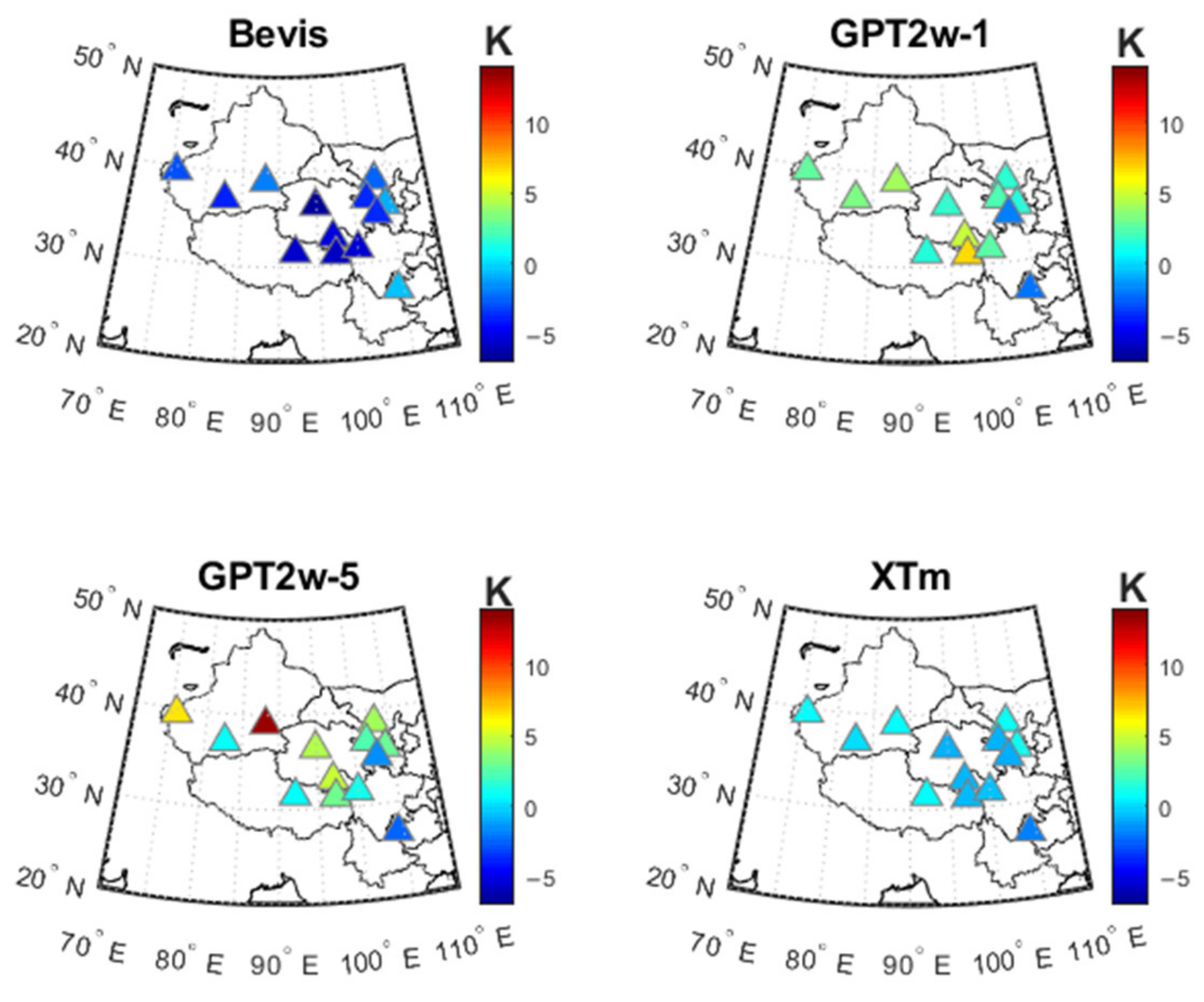
Figure 5 shows the bias distribution of four Tm models at the modeling station in 2018–2019. From
Figure 5, it can be seen that compared with the Tm reference values of the 13 modeling stations, the Tm values predicted by the Bevis model were generally smaller in the Qinghai–Tibet Plateau region, the predicted Tm values of the GPT2w-1 and GPT2w-5 models were smaller in specific areas of the southern and eastern Qinghai–Tibet Plateau, and the predicted Tm values of the GPT2w-1 and GPT2w-5 models were larger in other areas. The bias values of the XTm model were distributed more evenly around zero in the Qinghai–Tibet Plateau region, without any stations exhibiting significantly large biases. The bias values of the XTm model at the modeling stations were noticeably more stable compared with the other three selected models.
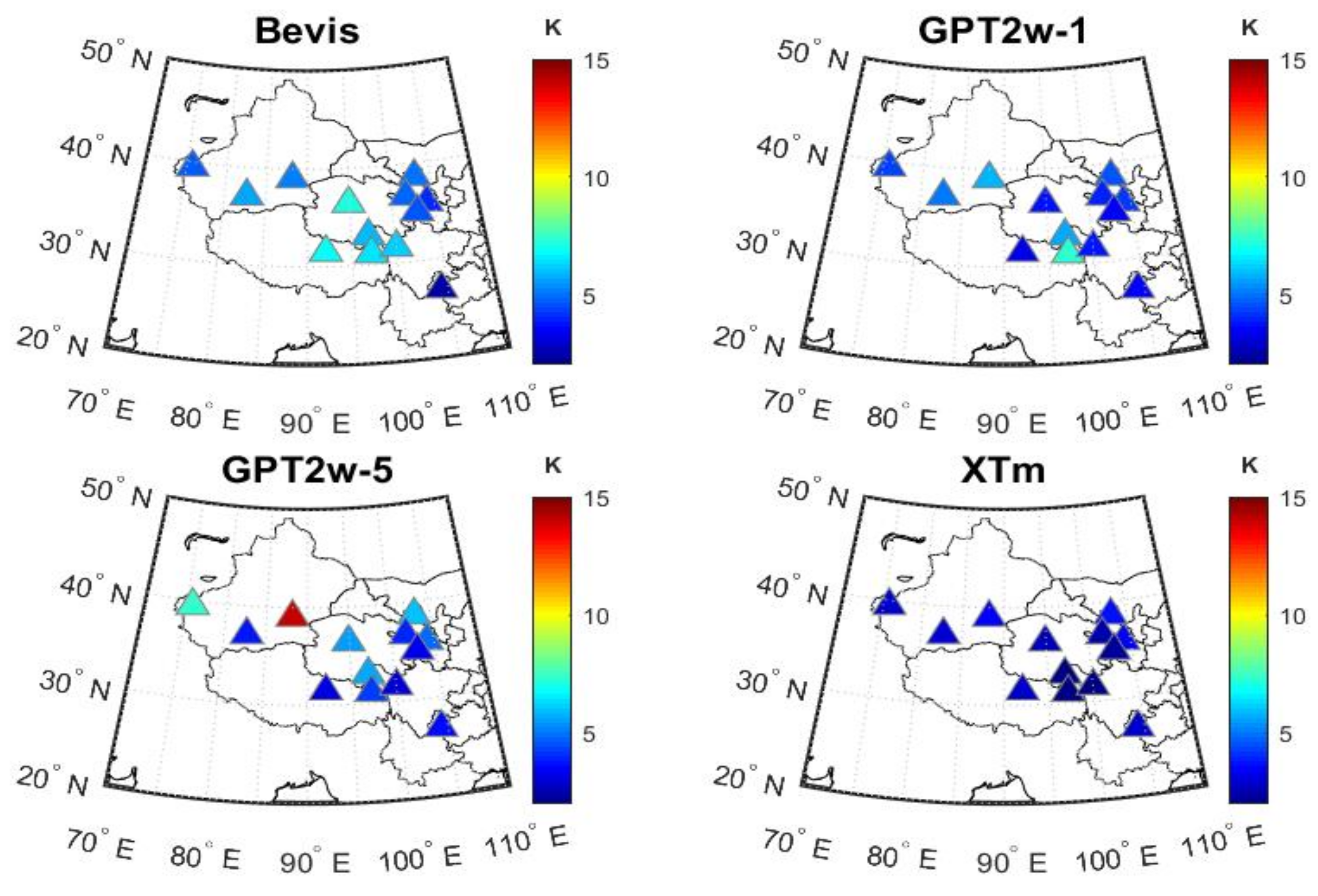
Figure 6 shows the RMS distribution of the four Tm models for the modeling stations in 2018–2019. In
Figure 6, it can be seen that the Bevis model exhibited larger RMS values in the central part of the Qinghai–Tibet Plateau, while the RMS values were relatively uniform around it. The GPT2w-1 model and GPT2w-5 model had extreme RMS values in the northwestern part of the Qinghai–Tibet Plateau. The XTm model, as proposed in this paper, demonstrated smaller RMS values in the Qinghai–Tibet Plateau region compared with the other specified models. It did not exhibit extreme maximum or minimum values, and the range of variation was the smallest, indicating that the new XTm model exhibited good stability.
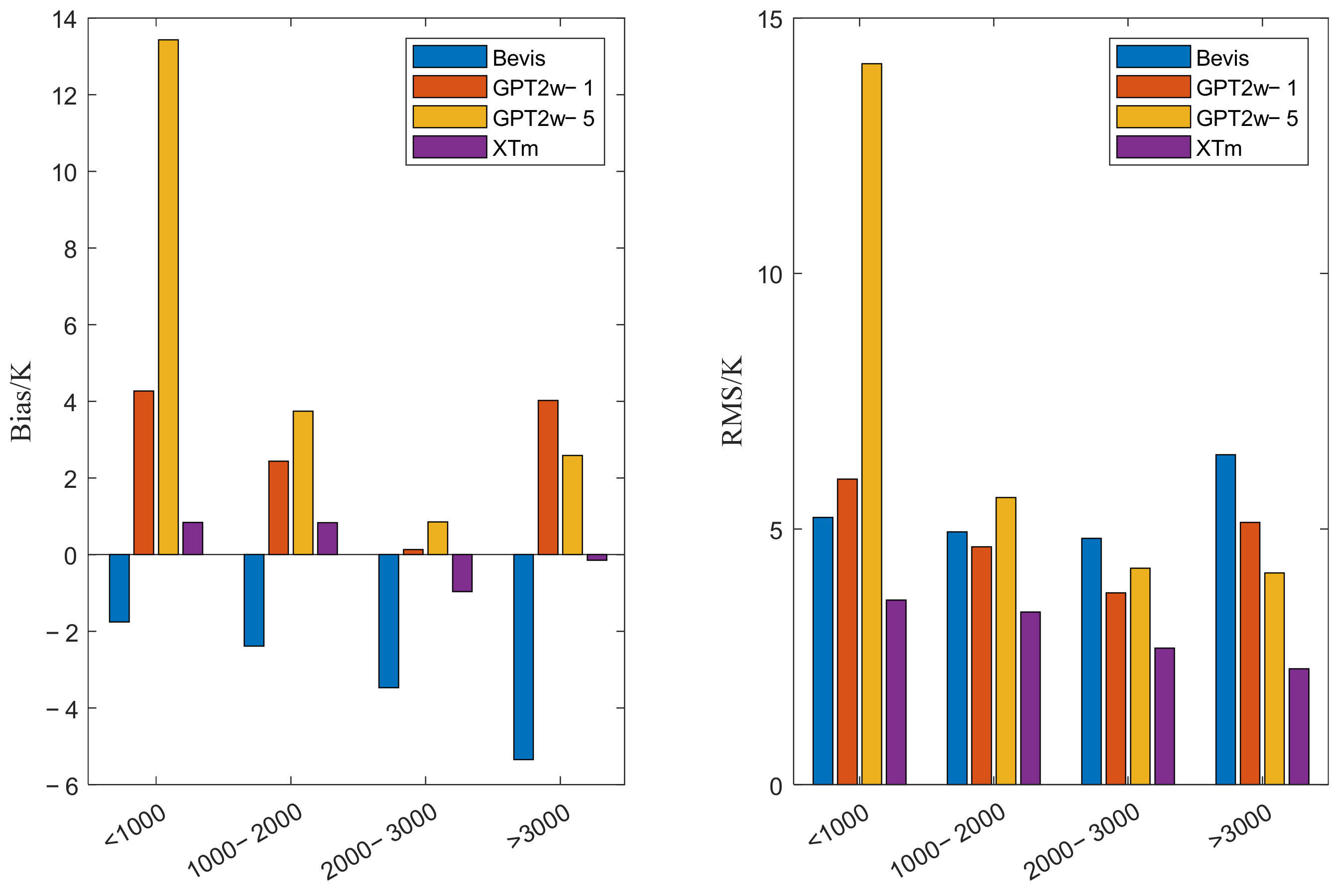
Given that the most prominent characteristic of the Qinghai–Tibet Plateau region is its large elevation range, as indicated in the above correlation analysis, there was a strong association between the Tm values and elevation. To analyze the relationship between the deviation and RMS calculated using different selected empirical models and the XTm model and the geopotential height, the 13 radiosonde stations were classified into intervals of 1000 m in elevation, which were categorized as <1000 m, 1000–2000 m, 2000–3000 m, and >3000 m, as shown in
Figure 7.
Figure 7 presents statistical histograms showing the bias and RMS values of different models calculated using the modeling radiosonde station data from 2018 to 2019 in the Qinghai–Tibet Plateau region as a function of the geopotential height. The Bevis model exhibited significant negative bias throughout the entire range of geopotential heights. As the geopotential height increased, the absolute value of the Bevis model’s bias became larger, indicating a growing systematic error with increasing geopotential height. This suggests that the Bevis model is not suitable for calculating the Tm in high-elevation areas. The GPT2w-1 model and GPT2w-5 model showed relatively small bias values in intervals of moderate elevation (1000–3000 m) compared with other ranges, but they exhibited substantial bias values at low or high geopotential heights. In areas with significant geopotential height variations, these models were not suitable. In contrast, the XTm model consistently displayed very low or even negligible bias values across different geopotential height intervals. When looking at the RMS, the GPT2w-5 model exhibited extremely high RMS values in the <1000 m geopotential height interval. The GPT2w-1 model showed RMS values that were very similar in the <1000 m and >3000 m geopotential height intervals, but they were higher than the RMS values in the areas (1000 m–3000 m). The Bevis model exhibited large RMS values in the >3000 m geopotential height interval. In contrast, the newly developed XTm model consistently demonstrated lower RMS values in each geopotential height interval compared with the other models. The RMS values for the XTm model fluctuated around 2.8 K, with a small variation range. In summary, across different geopotential height intervals, the deviation and RMS values of the new XTm model were consistently lower than those of other Tm models. This further indicates that the new XTm model performs well in terms of quality and stability in the Qinghai–Tibet Plateau region and can be applied in this region for extended periods.
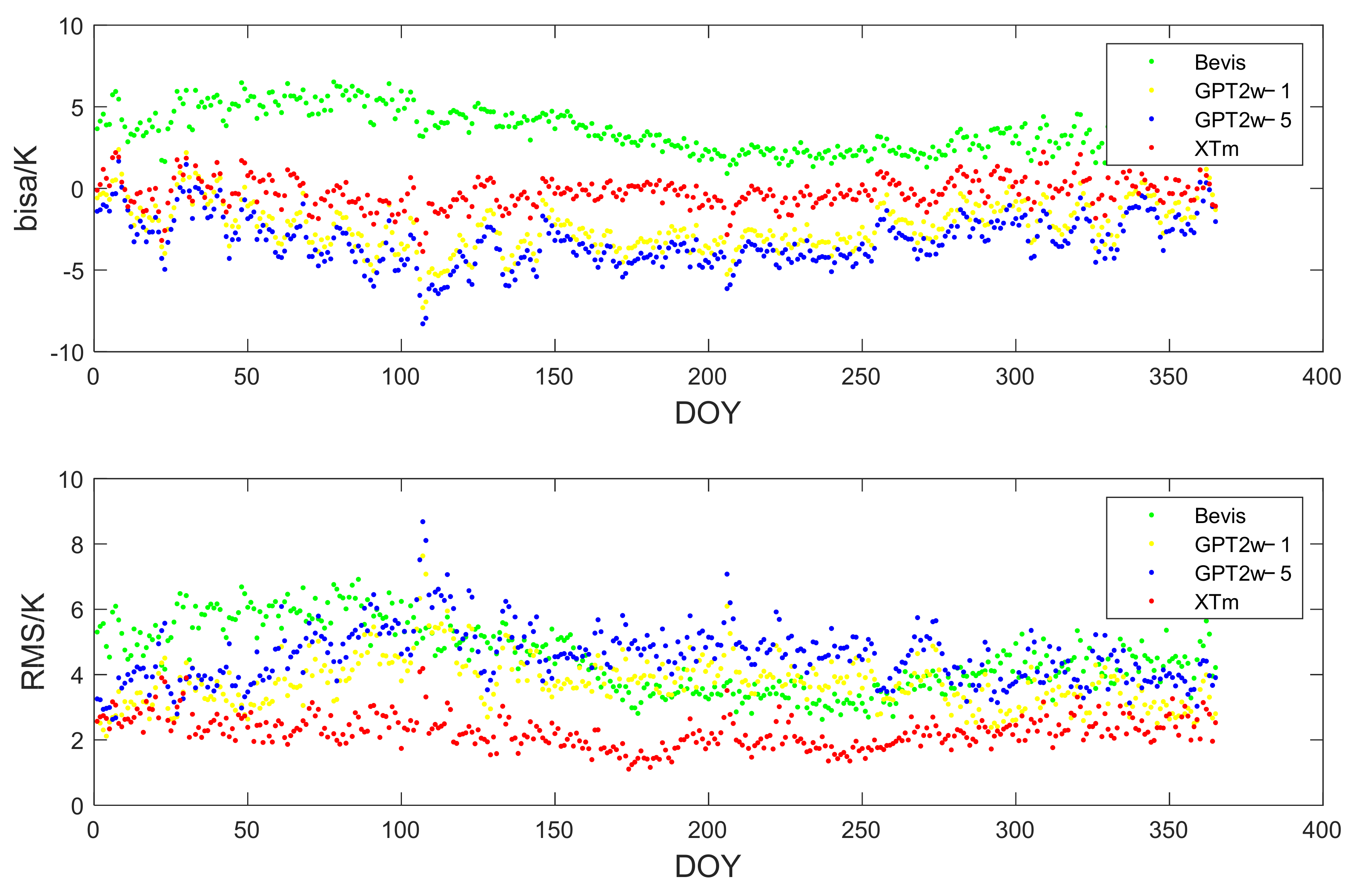
To assess the seasonal performance of the four selected models, this study calculated the daily deviation and RMS values for these models. The results are shown in
Figure 8. It can be observed that the GPT2w-1 model and GPT2w-5 model exhibited significant negative deviations for most days in the Qinghai–Tibet Plateau in 2018–2019, with peak deviations occurring in the spring. This further indicates that the GPT2w models have noticeable systematic errors. The Bevis model consistently showed relatively significant positive deviations throughout the year in the Qinghai–Tibet Plateau region. In contrast, the XTm model displayed smaller deviations for most periods, with negative deviations in the spring and winter and positive deviations in the summer and autumn. The deviations fluctuated around zero, and there was no significant seasonal variation. Regarding the RMS values, these models all exhibited relatively pronounced seasonal changes, with the RMS reaching peak values in the spring and relatively stable values in the summer. The Bevis model showed prominent RMS values in the winter as well, while the GPT2w-1 model exhibited higher RMS values in the summer. The GPT2w-5 model maintained stable values around 4 K across the entire Qinghai–Tibet Plateau region, except for summer, when it drops to around 1 K. In contrast, the XTm model consistently had values centered around 2 K, with lower RMS values in the summer, approaching 1 K. In summary, the XTm model exhibited smaller and more stable deviations and RMS values compared with the other selected Tm models, as it took into account annual and semi-annual variations. The quality of the XTm model was less affected by seasonal changes than the other Tm models.
3.2. Quality Analysis of Non-Modeling Station Sounding Data
Using the radiosonde data from non-modeling stations in the Qinghai–Tibet Plateau region for the years 2018–2019, the Tm values were calculated for each model. The Tm values obtained through numerical integration from the radiosonde data were used as the reference values. The quality of the XTm model was verified by calculating the bias and RMS values for the four specified models. The results are presented in
Table 3 and
Figure 9 and
Figure 10.
Table 3 displays the bias and RMS values for the four different Tm models for the non-modeling radiosonde stations in the Qinghai–Tibet Plateau region for the years 2018–2019. From
Table 3, it can be observed that the Bevis model exhibited a negative bias in the Qinghai–Tibet Plateau region, with an average bias of −3.91 K and a range of −6.33 K to −2.20 K. The bias values for the GPT2w-1 model and GPT2w-5 model were relatively close for the remaining stations, but the GPT2w-5 model had a larger range of variation, from 1.19 K to 6.85 K, with an average bias of 3.24 K, while the GPT2w-1 model had an average bias of 3.29 K, with a slightly smaller range of variation, indicating greater stability. This suggests that in all cases, both the Bevis model and the GPT2w models had systematic biases in calculating the Tm values in the Qinghai–Tibet Plateau region. The XTm model exhibited both negative and positive biases for the remaining stations, with a minimum bias of −0.43 K, a maximum bias of 1.14 K, and an average bias of 0.58 K when predicting the Tm values from non-modeling station sounding data. The bias values for the XTm model oscillated around zero, indicating no significant systematic bias. Furthermore, the Bevis model predicted Tm with the most significant RMS values, with an average RMS of 5.37 K, while the GPT2w-5 model exhibited the highest RMS values, reaching 7.9 K, with an average RMS of 4.89 K. The GPT2w-1 model had an average RMS of 4.78 K, similar to the GPT2w-5 model but with a smaller range of variation, ranging from 4.14 K to 5.33 K. The quality of the GPT2w-1 model was superior to that of the GPT2w-5 model, and the quality of the GPT2w-5 model was higher than that of the Bevis model, while the XTm model’s quality surpassed that of the GPT2w-1 model. The XTm model had the smallest average RMS value of 2.78 K compared with other models, with a 48% improvement over the Bevis model, a 43% improvement over the GPT2w-5 model, and a 42% improvement over the GPT2w-1 model. In summary, compared with other selected models in the Qinghai–Tibet Plateau, the XTm model exhibited the highest predictive quality, with the smallest bias and RMS variations, and it demonstrated stronger model stability.
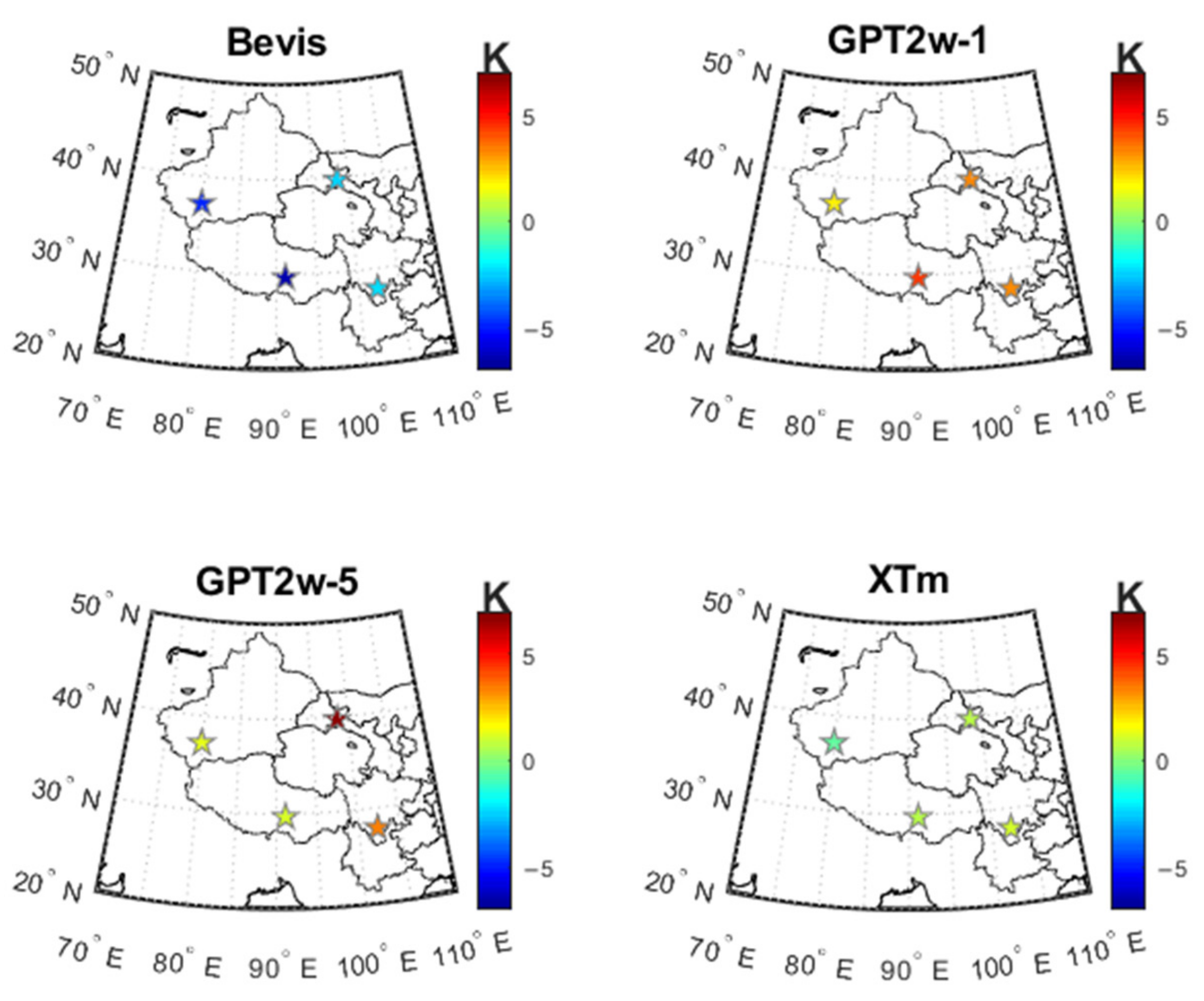
Figure 9 displays the distribution of the biases for the four different Tm models for non-modeling stations in the Qinghai–Tibet Plateau region for the years 2018–2019. From
Figure 9, it can be observed that the Bevis model exhibited negative bias across the entire Qinghai–Tibet Plateau region, with a negative bias approaching −7 K. Both the GPT2w-1 model and GPT2w-5 model showed positive biases at the non-modeling stations, with maximum biases nearing 5 K and 7 K, respectively. The XTm model’s bias values at non-modeling stations exhibited both negative and positive biases, but they were uniformly distributed around zero, with no significant bias at any station. The XTm model’s bias values at non-modeling stations were noticeably smaller and more stable compared with the other three selected XTm models.
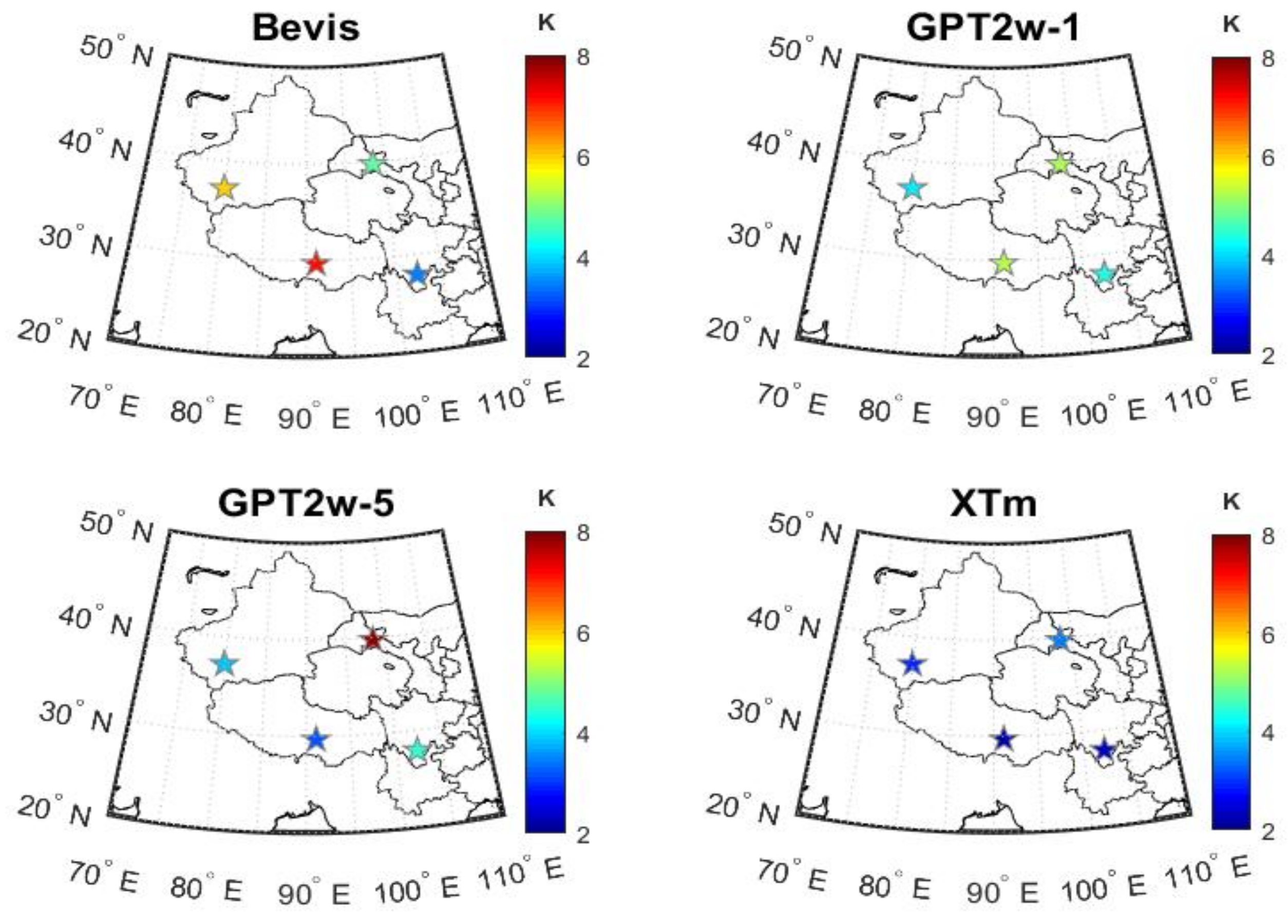
Figure 10 displays the distribution of RMS values for the four different Tm models at non-modeling stations in the Qinghai–Tibet Plateau region for the years 2018–2019. In
Figure 10, it can be observed that the Bevis model and GPT2w-1 model could exhibit relatively large RMS values in the southwestern part of the Qinghai–Tibet Plateau, while RMS values around other regions remained relatively uniform and around 5 K. The GPT2w-5 model, on the other hand, could show significant RMS peaks in the northeastern part of the plateau. The XTm model, as mentioned in the text, exhibited smaller RMS values at all non-modeling stations compared with the other specified models. There were no extreme RMS values, and the variation range was minimal, hovering around 3 K, indicating that the newly developed XTm model demonstrated good stability.
3.3. The Influence of Tm on PWV Calculations
The construction of a new model in the Qinghai–Tibet Plateau region aimed to enhance the predictive quality of the Tm. The Tm is a crucial parameter for converting the ZWD (zenith wet delay) into atmospheric precipitable water, but there is a lack of complete overlap between global GNSS stations and radiosonde stations. Additionally, most GNSS stations do not have matching sensors for meteorological observations. Therefore, it is challenging to thoroughly investigate the influence of the Tm on GNSS-derived atmospheric water vapor content from various angles and directions. Consequently, based on the conclusions regarding the impact of the Tm on GNSS-PWV from the literature [
17], the results were calculated using Equation (10), and a discussion and analysis were conducted:
RMSpwv is defined as the RMS value for the derived atmospheric water vapor, RMS
Π is defined as the RMS error, RMS
Tm is defined as the RMS error for the weighted average temperature, and RMSpwv/PWV is defined as the relative error for the derived atmospheric water vapor, with the Tm and PWV being averaged annually for the calculations. The computed values for each model in the Qinghai–Tibet Plateau region are shown in
Table 4 and
Figure 11.
The numbers shown in
Table 4 display the calculated RMSpwv values and RMSpwv/PWV values using observed data from radiosonde stations in 2018–2019.
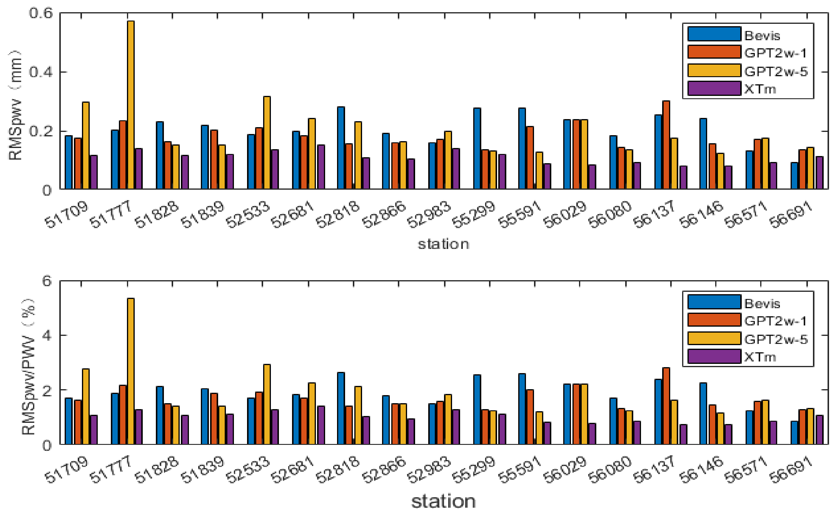
Figure 11 represents the RMSpwv values and RMSpwv/PWV values obtained for different stations corresponding to the four specified models. From
Table 4 and
Figure 11, it can be observed that the Bevis model and the GPT2w-5 model had the same average RMSpwv value of 0.21 mm in the Qinghai–Tibet Plateau region. However, their corresponding average RMSpwv/PWV values were different, with values of 1.94% and 1.96%, respectively. Except for the newly developed XTm model, all other models exhibited maximum values at different stations. The maximum RMSpwv values for these models were 0.28 mm, 0.30 mm, and 0.57 mm, and the maximum RMSpwv/PWV values were 2.62%, 2.82%, and 5.34%, respectively. The histograms for the stations also indicate that higher RMSpwv values correspond to larger RMSpwv/PWV values. The GPT2w-5 model showed the largest range in both the RMSpwv values and RMSpwv/PWV values, ranging from 0.13 mm to 0.57 mm and from 1.17% to 5.34%, respectively. In the case of the XTm model, all stations in the Qinghai–Tibet Plateau region had RMSpwv values below 0.15 mm, with an average RMSpwv value of 0.11 mm. The relative error in the PWV for this model had an average value of 1.03% and ranged from 0.74% to 1.40%. Compared with other models, the XTm model exhibited smaller variations and lower values in both the RMSpwv and RMSpwv/PWV, indicating that the errors between the Tm predicted by the XTm model and the reference values had a smaller and less variable impact on the PWV calculations. This suggests that the XTm model provides more accurate Tm values for the Qinghai–Tibet Plateau region.
4. Discussion
In this work, the XTm model was developed by considering a combination of factors, including the geopotential height above stations over the Qinghai–Tibet Plateau region, annual variations, semi-annual variations, surface temperature, and natural logarithm of water vapor pressure. During the establishment of the XTm model, it demonstrated strong predictive capabilities for the spatiotemporal variations of the Tm and its related factors. In this study, the XTm model, along with other selected Tm models, were used for quality validation. As indicated by the results in
Section 5, the XTm model can be employed with high precision in the Qinghai–Tibet Plateau region. Several reasons contributed to the improvements offered by the XTm model relative to other selected Tm models, as shown below.
First, the data used for the XTm model in this study were derived from atmospheric profiles measured using radiosonde water vapor measurements. On the other hand, the GPT2w model was developed based on data from ERA Interim (European Centre for Medium-Range Weather Forecasts), and these two data sources differ to some extent. These differences led to variations between the GPT2w model and the XTm model. Furthermore, the GPT2w model takes into account the geographical locations of the stations and effectively simulates the seasonal variations in the Tm. However, the Tm forecasts are significantly correlated with meteorological factors, and the GPT2w model does not consider this correlation. As a result, the GPT2w model does not achieve high quality in predicting the Tm over the Qinghai–Tibet Plateau. In contrast, the XTm model outperformed the GPT2w model in the Qinghai–Tibet Plateau.
Additionally, the Bevis model only considers the linear correlation between the Tm and Ts, which results in lower prediction quality in localized regions. In contrast with the Bevis model, the XTm model takes into account not only the ground temperature but also the water vapor pressure, geopotential height, annual variations, and semi-annual variations. This was precisely why the Bevis model exhibited larger biases and RMS values than the XTm model, especially in regions with higher geopotential heights, as shown in
Figure 7. The XTm model demonstrated higher quality across different geopotential heights and maintained a more even distribution. The results indicate that the XTm model performs significantly better than the Bevis model in various geopotential height regions of the Qinghai–Tibet Plateau.
Lastly, compared with models established by other researchers for the Qinghai–Tibet Plateau region based on linear correlations, the model proposed in this study took into account the meteorological factors with the highest correlation coefficients at the selected stations. These factors included the ground temperature, natural logarithm of water vapor pressure, and geopotential height. The quality of the fitted model was comparable with that of models developed by others in the region. Therefore, the XTm model can be used for Tm value predictions in this area.
5. Conclusions
We utilized radiosonde observations from 2008 to 2017 at 13 selected modeling stations within the Qinghai–Tibet Plateau region. It analyzed the correlations between Tm and its influencing factors. The analysis revealed that the Tm had a positive correlation with the ground temperature and natural logarithm of water vapor pressure, while it had a negative correlation with the geopotential height. Then, the XTm model was constructed using the nonlinear least squares method by taking into account the surface temperature, natural logarithm of water vapor pressure, geopotential height, and seasonal variations in the Qinghai–Tibet Plateau region. The relevant conclusions were as follows:
(1) We analyzed the predictive quality of the XTm model using radiosonde observations from 13 modeling stations in the Qinghai–Tibet Plateau region from 2018 to 2019. The model showed an average bias of −0.02 K and a mean RMS value of 2.83 K, which were both smaller and exhibited less variability compared with the Bevis model, GPT2w-1 model, and GPT2w-5 model in the same region. This indicates that the XTm model is more suitable for the Qinghai–Tibet Plateau region compared with other global empirical models.
(2) To validate the predictive capability of the XTm model at non-modeling sites in the Qinghai–Tibet Plateau, observations from four additional non-modeling radiosonde stations in 2018–2019 were selected for verification. The obtained bias and RMS values were 0.58 and 2.78 K, respectively. This shows that the XTm model also exhibited good prediction ability at non-modeling sites, and thus, it can be widely used in the region for Tm value predictions.
(3) By discussing the impact of the weighted average temperature calculated using different selected models based on GNSS-PWV inference, we could obtain the average values of RMSPWV and RMSPWV/PWV for the XTm model, which were 0.11 mm and 1.03%, respectively. Compared with the other three selected models, the XTm model exhibited smaller RMS values. Therefore, the predictive capability of the XTm model was superior to the other selected models.
In summary, the XTm model could provide high-precision Tm values for GNSS-PWV inversion, and high-precision GNSS-PWV is of great significance for weather forecasting and extreme weather research.
Author Contributions
Conceptualization, B.Z., K.T. and S.X.; methodology, B.Z. and K.T.; investigation, B.G.; formal analysis, B.H.; writing—original draft preparation, Z.W.; data curation, K.T; writing—review and editing. All authors have read and agreed to the published version of the manuscript.
Funding
This work was supported by the National Natural Science Foundation of China (NSFC, 41974007); Key Scientific and Technological Research Project of Henan Province (grant no. 232102320280); the Key Laboratory of Geospace Environment and Geodesy, Ministry of Education, Wuhan University (21-01-05); Natural Science Foundation of Shandong Youth Fund (ZR2022QD144), Shandong Provincial Department of Science and Technology; Doctoral Research Initiation Fund of Shandong University of Technology (05827); Hubei University of Science and Technology 2023 First Batch of Doctoral Research Initiation Project (Si Xiong) and Scientific Innovation Project for Young Scientists in Shandong Provincial Universities (2022KJ224).
Institutional Review Board Statement
Not applicable.
Informed Consent Statement
Not applicable.
Data Availability Statement
Conflicts of Interest
The authors declare no conflict of interest.
Appendix A
The station information relating to
Figure 1.
| Name | Latitude (°) | Longitude (°) | Elevation (m) |
| CHM00051709 | 39.4833 | 75.75 | 1386.7 |
| CHM00051777 | 39.0333 | 88.1667 | 889 |
| CHM00051839 | 37.0667 | 82.7167 | 1409 |
| CHM00052681 | 38.6333 | 103.0833 | 1367 |
| CHM00052818 | 36.4167 | 94.9 | 2809 |
| CHM00052866 | 36.7167 | 101.75 | 2296 |
| CHM00052983 | 35.8667 | 104.15 | 1875 |
| CHM00055299 | 31.4833 | 92.0667 | 4508 |
| CHM00056029 | 33 | 96.95 | 3716.9 |
| CHM00056080 | 35 | 102.9 | 2910 |
| CHM00056137 | 31.15 | 97.1667 | 3307 |
| CHM00056146 | 31.6167 | 100 | 3394 |
| CHM00056691 | 26.8667 | 104.2833 | 2236 |
| CHM00051828 | 37.1333 | 79.9333 | 1375 |
| CHM00052533 | 39.7667 | 98.4833 | 1478 |
| CHM00055591 | 29.6667 | 91.1333 | 3650 |
| CHM00056571 | 27.9 | 102.2667 | 1599 |
References
- Huang, L.; Liu, W.; Mo, Z.; Zhang, H.; Li, J.; Chen, F.; Liu, L.; Jiang, W. A new model for vertical adjustment of precipitable water vapor with consideration of the time-varying lapse rate. GPS Solut. 2023, 27, 170. [Google Scholar] [CrossRef]
- Yao, Y.; Zhang, S.; Kong, J. Progress and Prospects in GNSS Space Environmental Research. Acta Geod. Cartogr. Sin. 2017, 46, 1408–1420. [Google Scholar]
- Mo, Z.; Huang, L.; Guo, X.; Huang, L.; Liu, L.; Pang, Z.; Deng, Y. Quality Analysis of GNSS Water Vapor Retrieval in Guilin Area Using ERA5 Data. J. Nanjing Univ. Inf. Sci. Technol. 2021, 13, 131–137. [Google Scholar]
- Mo, Z.; Li, X.; Huang, L.; Liu, L.; Wei, X.; Zhou, Q. Refinement of Atmospheric Weighted Average Temperature Model Considering Multiple Factors in Western China. J. Geod. Geodyn. 2021, 41, 145–151. [Google Scholar]
- Huang, L.; Wu, P.; Wang, H.; Liu, L. Refinement of GPS Atmospheric Water Vapor Conversion Coefficient Model in Southwest China. J. Geod. Geodyn. 2019, 39, 256–261. [Google Scholar] [CrossRef]
- Huang, L.; Liu, L.; Chen, H.; Jiang, W. An improved atmospheric weighted mean temperature model and its impact on GNSS precipitable water vapor estimates for China. GPS Solut. 2019, 23, 51. [Google Scholar] [CrossRef]
- Bevis, M.; Businger, S.; Chiswell, S.; Herring, T.A.; Anthes, R.A.; Rocken, C.; Ware, R.H. GPS meteorology: Mapping zenith wet delays onto precipitable water. J. Appl. Meteorol. 1994, 33, 379–386. [Google Scholar] [CrossRef]
- Böhm, J.; Möller, G.; Schindelegger, M.; Pain, G.; Weber, R. Development of an improved empirical model for slant delay sinthe troposphere(GPT2w). GPS Solut. 2015, 2015, 433–441. [Google Scholar] [CrossRef]
- Baldysz, Z.; Nykiel, G. Improved Empirical Coefficients for Estimating Water Vapor Weighted Mean Temperature over Europe for GNSS Applications. Remote Sens. 2019, 11, 1995. [Google Scholar] [CrossRef]
- Huang, L.; Peng, H.; Liu, L.; Li, C.; Kang, C.; Xie, S. An Atmospheric Weighted Average Temperature Model for China Considering Vertical Gradients. Acta Geod. Cartogr. Sin. 2020, 49, 432–442. [Google Scholar]
- Huang, L.; Fang, X.; Zhang, T.; Wang, H.; Cui, L.; Liu, L. Evaluation of surface temperature and pressure derived from MERRA-2 and ERA5 reanalysis datasets and their applications in hourly GNSS precipitable water vapor retrieval over China. Geod. Geodyn. 2022, 14, 111–120. [Google Scholar] [CrossRef]
- Yao, C.; Luo, Z.; Liu, L.; Zhou, B. Study on the Relationship Between Terrain and Wet Delay and Precipitable Water Conversion in Low-Latitude Areas of China. J. Wuhan Univ. 2015, 40, 907–912. [Google Scholar]
- Li, L.; Fan, Y.; Wang, L.; Tian, Y.; Jiang, T.; Song, T.; Yi, J. Analysis and Modeling of Factors Influencing Weighted Average Temperature in Hunan Region. J. Geod. Geodyn. 2018, 38, 48–52. [Google Scholar]
- Huang, L.; Liu, Z.; Peng, H.; Xiong, S.; Zhu, G.; Chen, F.; Liu, L.; He, H. A novel global grid model for atmospheric weighted mean temperature in real-time GNSS precipitable water vapor sounding. IEEE J. Sel. Top. Appl. Earth Obs. Remote Sens. 2023, 16, 3322–3335. [Google Scholar] [CrossRef]
- Zhang, B.; Guo, Z.; Lin, F.; Peng, C.; Jiang, D. Establishment and quality Evaluation of Weighted Average Temperature Models in Guangxi Region. J. Xinyang Norm. Univ. 2022, 35, 85–91. [Google Scholar]
- Li, J.; Mao, J.; Li, C.; Xia, Q. Regression Analysis of Water Vapor Distribution in Eastern China Using GPS Remote Sensing and Weighted “Average Temperature”. Acta Meteorol. Sin. 1999, 57, 283–292. [Google Scholar]
- Huang, L.; Jiang, W.; Liu, L.; Chen, H.; Ye, S. A new global grid model for the determination of atmospheric weighted mean temperature in GPS precipitable water vapor. J. Geod. 2019, 93, 159–176. [Google Scholar] [CrossRef]
- Huang, L.; Mo, Z.; Xie, S.; Liu, L.; Chen, J.; Kang, C.; Wang, S. Spatiotemporal characteristics of GNSS-derived precipitable water vapor during heavy rainfall events in Guilin, China. Satell. Navig. 2021, 2, 13. [Google Scholar] [CrossRef]
- Huang, L.; Mo, Z.; Liu, L.; Zeng, Z.; Chen, J.; Xiong, S.; He, H. Evaluation of Hourly PWV Products Derived from ERA5 and MERRA-2 over the Tibetan Plateau Using Ground- Based GNSS Observations by Two Enhanced Models. Earth Space Sci. 2021, 8, e2020EA001516. [Google Scholar] [CrossRef]
- Yao, Y.; Zhang, B.; Xu, C.; Yan, F. Improved one/multi-parameter models that consider seasonal and geographic variations for estimating weighted mean temperature in ground-based GPS meteorology. J. Geod. 2014, 88, 273–282. [Google Scholar] [CrossRef]
Figure 1.
Distribution map of stations on the Qinghai–Tibet Plateau. The yellow circles denote the positions of the 13 modeling stations, and the red triangles denote the positions of the 4 non-modeling stations.
Figure 1.
Distribution map of stations on the Qinghai–Tibet Plateau. The yellow circles denote the positions of the 13 modeling stations, and the red triangles denote the positions of the 4 non-modeling stations.
Figure 2.
Diagram of linear correlation between Ts and Tm.
Figure 2.
Diagram of linear correlation between Ts and Tm.
Figure 3.
Diagram of linear correlation between ln(e) and Tm.
Figure 3.
Diagram of linear correlation between ln(e) and Tm.
Figure 4.
Diagram of linear correlation between H and Tm.
Figure 4.
Diagram of linear correlation between H and Tm.
Figure 5.
Scatter plot for evaluating the deviation of various Tm models using radiosonde data from modeling stations from 2018 to 2019.
Figure 5.
Scatter plot for evaluating the deviation of various Tm models using radiosonde data from modeling stations from 2018 to 2019.
Figure 6.
Scatter plot of root-mean-square error of each Tm model evaluated using radiosonde data from modeling stations from 2018 to 2019.
Figure 6.
Scatter plot of root-mean-square error of each Tm model evaluated using radiosonde data from modeling stations from 2018 to 2019.
Figure 7.
The statistical histogram of error variation of Tm models with high potential was evaluated by using the 2018–2019 radiosonde data from modeling stations (the left one refers to bias and the right one to RMS).
Figure 7.
The statistical histogram of error variation of Tm models with high potential was evaluated by using the 2018–2019 radiosonde data from modeling stations (the left one refers to bias and the right one to RMS).
Figure 8.
Statistical scatter chart of seasonal error evaluation for each Tm model using 2018–2019 modeling station radiosonde data.
Figure 8.
Statistical scatter chart of seasonal error evaluation for each Tm model using 2018–2019 modeling station radiosonde data.
Figure 9.
Evaluation of scatter points in the deviation of various Tm models using non-modeling station radiosonde data from 2018 to 2019.
Figure 9.
Evaluation of scatter points in the deviation of various Tm models using non-modeling station radiosonde data from 2018 to 2019.
Figure 10.
Scatter plot of root-mean-square error of each Tm model evaluated using non-modeling station radiosonde data from 2018 to 2019.
Figure 10.
Scatter plot of root-mean-square error of each Tm model evaluated using non-modeling station radiosonde data from 2018 to 2019.
Figure 11.
The RMSpwv values and RMSpwv/PWV values obtained for 17 radiosonde stations corresponding to the four specified models from 2018 to 2019.
Figure 11.
The RMSpwv values and RMSpwv/PWV values obtained for 17 radiosonde stations corresponding to the four specified models from 2018 to 2019.
Table 1.
XTm model coefficients calculated using radiosonde data from 2008 to 2017 in the Qinghai–Tibet Plateau.
Table 1.
XTm model coefficients calculated using radiosonde data from 2008 to 2017 in the Qinghai–Tibet Plateau.
| Coefficients | Fitted Values |
|---|
| 157.912 ± 0.843 |
| 0.389 ± 0.003 |
| 3.300 ± 0.036 |
| −0.00138 ± 0.00002 |
| −1.266 ± 0.055 |
| −1.037 ± 0.032 |
| 0.156 ± 0.028 |
| 0.046 ± 0.027 |
Table 2.
Statistical table for evaluation various Tm models using the 13 sets of radiosonde data of modeling stations from 2018 to 2019 as reference.
Table 2.
Statistical table for evaluation various Tm models using the 13 sets of radiosonde data of modeling stations from 2018 to 2019 as reference.
| Models | Bias/K | RMS/K |
|---|
| Min | Max | Average | Min | Max | Average |
|---|
| Bevis | −6.39 | −0.37 | −3.58 | 2.45 | 7.23 | 5.39 |
| GPT2w-1 | −1.96 | 6.82 | 2.35 | 3.38 | 7.44 | 4.62 |
| GPT2w-5 | −2.29 | 13.43 | 3.24 | 3.14 | 14.11 | 5.39 |
| XTm | −1.72 | 1.15 | −0.02 | 2.00 | 3.85 | 2.83 |
Table 3.
Statistical table for evaluation of various Tm models using the radiosonde data of non-modeling stations from 2018 to 2019 as reference.
Table 3.
Statistical table for evaluation of various Tm models using the radiosonde data of non-modeling stations from 2018 to 2019 as reference.
| Models | Bias/K | RMS/K |
|---|
| Min | Max | Average | Min | Max | Average |
|---|
| Bevis | −6.33 | −2.20 | −3.91 | 3.51 | 7.17 | 5.37 |
| GPT2w-1 | 1.89 | 4.50 | 3.29 | 4.14 | 5.33 | 4.78 |
| GPT2w-5 | 1.19 | 6.85 | 3.24 | 3.23 | 7.90 | 4.89 |
| XTm | −0.43 | 1.14 | 0.58 | 2.25 | 3.48 | 2.78 |
Table 4.
The RMS error and theoretical relative error of PWV were calculated by using the measured data of the 17 radiosonde stations in 2018–2019.
Table 4.
The RMS error and theoretical relative error of PWV were calculated by using the measured data of the 17 radiosonde stations in 2018–2019.
| Model | RMSPWV/mm | RMSPWV/PWV% |
|---|
| Min | Max | Average | Min | Max | Average |
|---|
| Bevis | 0.16 | 0.28 | 0.21 | 0.88 | 2.62 | 1.94 |
| GPT2w-1 | 0.14 | 0.30 | 0.18 | 1.27 | 2.82 | 1.72 |
| GPT2w-5 | 0.13 | 0.57 | 0.21 | 1.17 | 5.34 | 1.96 |
| XTm | 0.08 | 0.15 | 0.11 | 0.74 | 1.40 | 1.03 |
| Disclaimer/Publisher’s Note: The statements, opinions and data contained in all publications are solely those of the individual author(s) and contributor(s) and not of MDPI and/or the editor(s). MDPI and/or the editor(s) disclaim responsibility for any injury to people or property resulting from any ideas, methods, instructions or products referred to in the content. |
© 2023 by the authors. Licensee MDPI, Basel, Switzerland. This article is an open access article distributed under the terms and conditions of the Creative Commons Attribution (CC BY) license (https://creativecommons.org/licenses/by/4.0/).


