
Reanalyzing Jupiter ISO/SWS Data through a More Recent Atmospheric Model
 , , , and
Abstract
:1. Introduction
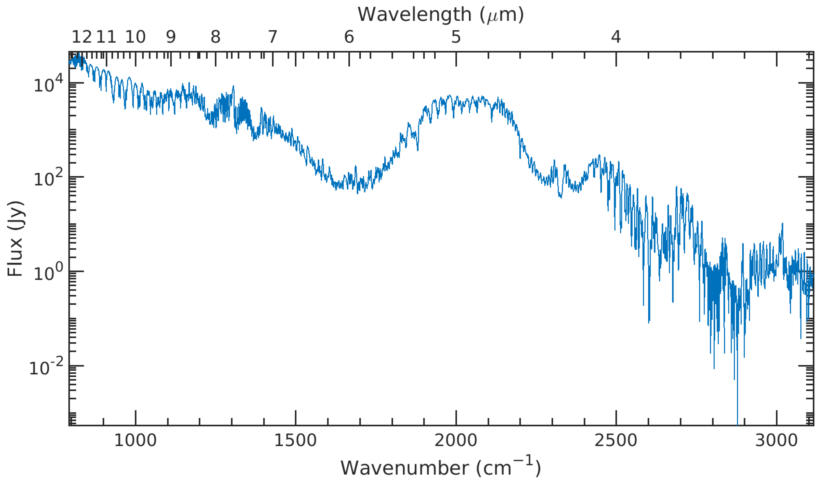
2. Observations
3. Methodology
3.1. NEMESIS Radiative Transfer Suite
3.2. Model Atmosphere
4. Results
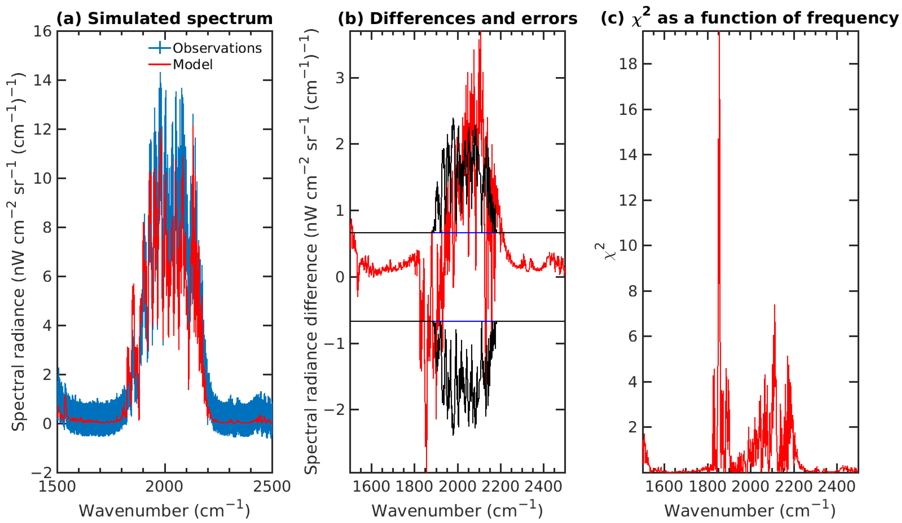
4.1. Best-Fitting Spectrum
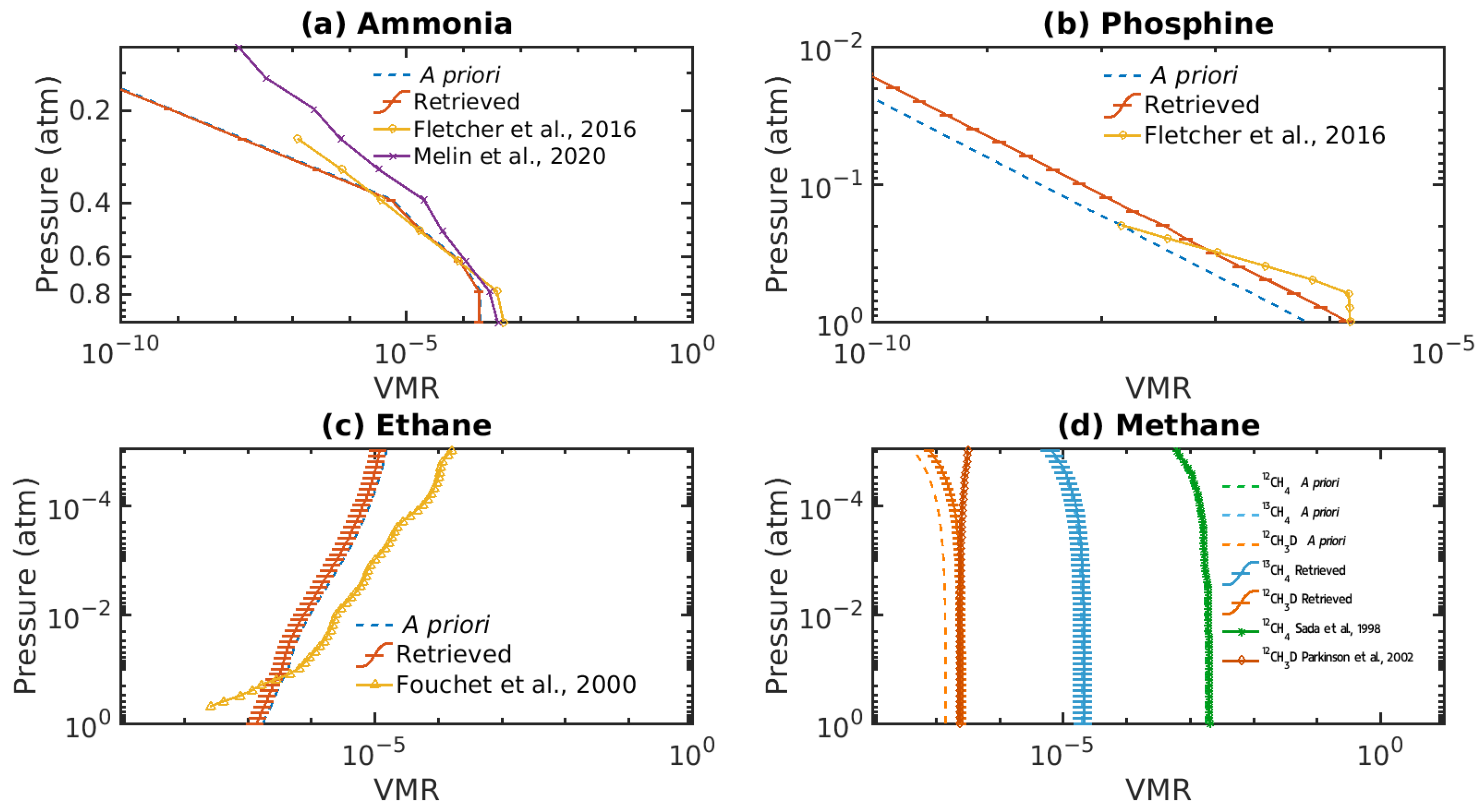
4.2. Retrieved Parameters
4.3. Sensitivity Analysis
5. Discussion
5.1. Temperature
5.2. Chemical Species
5.3. Isotopic Ratios
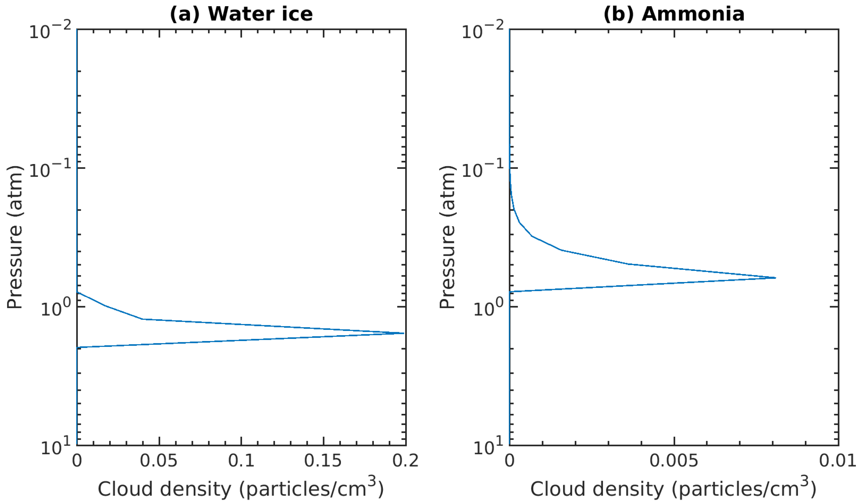
5.4. Aerosols
6. Conclusions
- We successfully obtained a simulated spectrum of the atmosphere of Jupiter with for the 793–1500 cm region;
- We retrieved a temperature profile that is colder than what is found in other published works for pressures higher than 0.1 atm;
- We retrieved various chemical species, obtaining an increase in abundance for PH and an increase for CH and CHD when compared with the a priori profiles;
- From the methane abundance profiles, we obtained a C/C ratio of 84 ± 27 and a D/H ratio of (3.5 ± 0.6) × 10, in good agreement with previous works;
- We successfully obtained a simulated spectrum of the atmosphere of Jupiter with for the 1500–2499 cm region;
- We retrieved an aerosol density profile for an NH cloud with a cloud base altitude at 6 ± 10 km and a fractional scale height of 0.3 ± 0.1;
Author Contributions
Funding
Institutional Review Board Statement
Informed Consent Statement
Data Availability Statement
Acknowledgments
Conflicts of Interest
Abbreviations
| ISO | Infrared Space Observatory |
| SWS | Short Wavelength Spectrometer |
| NEMESIS | Non-linear Optimal Estimator for MultivariatE Spectral analySIS |
| CIRS | Composite Infrared Spectrometer |
| IRTF | Infrared Telescope Facility |
| TEXES | Texas Echelon Cross Echelle Spectrograph |
| JIRAM | Jovian Infrared Auroral Mapper |
| JUICE | Jupiter Icy Moons Explorer |
| VMR | Volume Mixing Ratio |
| FOV | Field of View |
References
- Kunde, V.; Hanel, R.; Maguire, W.; Gautier, D.; Baluteau, J.P.; Marten, A.; Chedin, A.; Husson, N.; Scott, N. The tropospheric gas composition of Jupiter’s north equatorial belt /NH3, PH3, CH3D, GeH4, H2O/ and the Jovian D/H isotopic ratio. Astrophys. J. 1982, 263, 443–467. [Google Scholar] [CrossRef]
- Sada, P.V.; McCabe, G.H.; Bjoraker, G.L.; Jennings, D.E.; Reuter, D.C. 13C-Ethane in the Atmospheres of Jupiter and Saturn. Astrophys. J. 1996, 472, 903. [Google Scholar] [CrossRef]
- Sada, P.V.; Bjoraker, G.L.; Jennings, D.E.; McCabe, G.H.; Romani, P.N. Observations of CH4, C2H6, and C2H2 in the Stratosphere of Jupiter. Icarus 1998, 136, 192–201. [Google Scholar] [CrossRef]
- Niemann, H.B.; Atreya, S.K.; Carignan, G.R.; Donahue, T.M.; Haberman, J.A.; Harpold, D.N.; Hartle, R.E.; Hunten, D.M.; Kasprzak, W.T.; Mahaffy, P.R.; et al. The composition of the Jovian atmosphere as determined by the Galileo probe mass spectrometer. J. Geophys. Res. Planets 1998, 103, 22831–22846. [Google Scholar] [CrossRef] [PubMed]
- Fouchet, T.; Lellouch, E.; Bézard, B.; Feuchtgruber, H.; Drossart, P.; Encrenaz, T. Jupiter’s hydrocarbons observed with ISO-SWS: Vertical profiles of C2H6 and C2H2, detection of CH3C2H. Astron. Astrophys. 2000, 355, L13–L17. [Google Scholar] [CrossRef]
- Parkinson, C.; Jaffel, L.; McConnell, J. Deuterium Abundance from HD and CH3D Reservoirs in the Atmosphere of Jupiter. Bull. Am. Astron. Soc. 2001, 33, 1042. [Google Scholar]
- Fletcher, L.N.; Greathouse, T.K.; Orton, G.S.; Sinclair, J.A.; Giles, R.S.; Irwin, P.G.J.; Encrenaz, T. Mid-infrared mapping of Jupiter’s temperatures, aerosol opacity and chemical distributions with IRTF/TEXES. Icarus 2016, 278, 128–161. [Google Scholar] [CrossRef]
- Pierel, J.D.R.; Nixon, C.A.; Lellouch, E.; Fletcher, L.N.; Bjoraker, G.L.; Achterberg, R.K.; Bézard, B.; Hesman, B.E.; Irwin, P.G.J.; Flasar, F.M. D/H Ratios on Saturn and Jupiter from Cassini CIRS. Astron. J. 2017, 154, 178. [Google Scholar] [CrossRef]
- Lellouch, E.; Bézard, B.; Fouchet, T.; Feuchtgruber, H.; Encrenaz, T.; de Graauw, T. The deuterium abundance in Jupiter and Saturn from ISO-SWS observations. Astron. Astrophys. 2001, 370, 610–622. [Google Scholar] [CrossRef]
- Melin, H.; Fletcher, L.N.; Irwin, P.G.J.; Edgington, S.G. Jupiter in the Ultraviolet: Acetylene and Ethane Abundances in the Stratosphere of Jupiter from Cassini Observations between 0.15 and 0.19 μm. Astron. J. 2020, 159, 291. [Google Scholar] [CrossRef]
- Lellouch, E.; Feuchtgruber, H.; de Graauw, T.; Encrenaz, T.; Bézard, B.; Griffin, M. Deuterium and Oxygen in Giant Planets. In Proceedings of the The First ISO workshop on Analytical Spectroscopy, Madrid, Spain, 6–8 October 1997; Heras, A.M., Leech, K., Trams, N.R., Perry, M., Eds.; ESA Special Publication: Noordwijk, The Netherlands, 1997; Volume 419, p. 131. [Google Scholar]
- Encrenaz, T.; Drossart, P.; Feuchtgruber, H.; Lellouch, E.; Bézard, B.; Fouchet, T.; Atreya, S. The atmospheric composition and structure of Jupiter and Saturn from ISO observations: A preliminary review. Planet. Space Sci. 1999, 47, 1225–1242. [Google Scholar] [CrossRef]
- Sánchez-López, A.; López-Puertas, M.; García-Comas, M.; Funke, B.; Fouchet, T.; Snellen, I.A.G. The CH4 abundance in Jupiter’s upper atmosphere. Astron. Astrophys. 2022, 662, A91. [Google Scholar] [CrossRef]
- Flasar, F.M.; Kunde, V.G.; Abbas, M.M.; Achterberg, R.K.; Ade, P.; Barucci, A.; Bézard, B.; Bjoraker, G.L.; Brasunas, J.C.; Calcutt, S.; et al. Exploring The Saturn System In The Thermal Infrared: The Composite Infrared Spectrometer. Space Sci. Rev. 2004, 115, 169–297. [Google Scholar] [CrossRef]
- Noschese, R.; Cicchetti, A.; Sordini, R.; Cartacci, M.; Mura, A.; Brooks, S.; Lastri, M.; Filacchione, G.; Migliorini, A.; Moriconi, M.; et al. Juno/JIRAM: Planning and commanding activities. Adv. Space Res. 2020, 65, 598–615. [Google Scholar] [CrossRef]
- Lacy, J.H.; Richter, M.J.; Greathouse, T.K.; Jaffe, D.T.; Zhu, Q. TEXES: A Sensitive High-Resolution Grating Spectrograph for the Mid-Infrared. Publ. Astron. Soc. Pac. 2002, 114, 153–168. [Google Scholar] [CrossRef]
- Kessler, M. The Infrared Space Observatory (ISO) mission. Adv. Space Res. 2002, 30, 1957–1965. [Google Scholar] [CrossRef]
- de Graauw, T.; Haser, L.; Beintema, D.; Roelfsema, P.; Agthoven, H.; Barl, L.; Bauer, O.; Bekenkamp, H.; Boonstra, A.J.; Boxhoorn, D.; et al. Observing with the ISO Short-Wavelength Spectrometer. Astron. Astrophys. 1996, 315, L49–L54. [Google Scholar]
- Encrenaz, T.; de Graauw, T.; Schaeidt, S.; Lellouch, E.; Feuchtgruber, H.; Beintema, D.A.; Bezard, B.; Drossart, P.; Griffin, M.; Heras, A.; et al. First results of ISO-SWS observations of Jupiter. Astron. Astrophys. 1996, 315, L397–L400. [Google Scholar]
- Roos-Serote, M.; Drossart, P.; Encrenaz, T.; Carlson, R.; Leader, F. Constraints on the Tropospheric Cloud Structure of Jupiter from Spectroscopy in the 5-μm Region: A Comparison between Voyager/IRIS, Galileo/NIMS, and ISO/SWS Spectra. Icarus 1999, 137, 315–340. [Google Scholar] [CrossRef]
- Irwin, P.; Teanby, N.; Kok, R.; Fletcher, L.; Howett, C.; Tsang, C.; Wilson, C.; Calcutt, S.; Nixon, C.; Parrish, P. The NEMESIS planetary atmosphere radiative transfer and retrieval tool. J. Quant. Spectrosc. Radiat. Transf. 2008, 109, 1136–1150. [Google Scholar] [CrossRef]
- Rodgers, C.D. Inverse Methods for Atmospheric Sounding; World Scientific: Singapore, 2000. [Google Scholar] [CrossRef]
- Irwin, P.; Parrish, P.; Fouchet, T.; Calcutt, S.; Taylor, F.; Simon-Miller, A.; Nixon, C. Retrievals of jovian tropospheric phosphine from Cassini/CIRS. Icarus 2004, 172, 37–49. [Google Scholar] [CrossRef]
- Fletcher, L.N.; Orton, G.S.; Sinclair, J.A.; Guerlet, S.; Read, P.L.; Antuñano, A.; Achterberg, R.K.; Flasar, F.M.; Irwin, P.G.J.; Bjoraker, G.L.; et al. A hexagon in Saturn’s northern stratosphere surrounding the emerging summertime polar vortex. Nat. Commun. 2018, 9, 3564. [Google Scholar] [CrossRef]
- Irwin, P.G.J.; Weir, A.L.; Smith, S.E.; Taylor, F.W.; Lambert, A.L.; Calcutt, S.B.; Cameron-Smith, P.J.; Carlson, R.W.; Baines, K.; Orton, G.S.; et al. Cloud structure and atmospheric composition of Jupiter retrieved from Galileo near-infrared mapping spectrometer real-time spectra. J. Geophys. Res. Planets 1998, 103, 23001–23022. [Google Scholar] [CrossRef]
- West, R.A.; Baines, K.H.; Friedson, A.J.; Banfield, D.; Ragent, B.; Taylor, F.W. Jovian clouds and haze. In Jupiter. The Planet, Satellites and Magnetosphere; Bagenal, F., Dowling, T.E., McKinnon, W.B., Eds.; Cambridge University Press: Cambridge, UK, 2004; Volume 1, pp. 79–104. [Google Scholar]
- Hale, G.M.; Querry, M.R. Optical Constants of Water in the 200-nm to 200-μm Wavelength Region. Appl. Opt. 1973, 12, 555–563. [Google Scholar] [CrossRef] [PubMed]
- Martonchik, J.V.; Orton, G.S.; Appleby, J.F. Optical properties of NH3 ice from the far infrared to the near ultraviolet. Appl. Opt. 1984, 23, 541–547. [Google Scholar] [CrossRef] [PubMed]
- Koukouli, M.; Irwin, P.; Taylor, F. Water vapor abundance in Venus’ middle atmosphere from Pioneer Venus OIR and Venera 15 FTS measurements. Icarus 2005, 173, 84–99. [Google Scholar] [CrossRef]
- Irwin, P.G.J.; Lellouch, E.; de Bergh, C.; Courtin, R.; Bézard, B.; Fletcher, L.N.; Orton, G.S.; Teanby, N.A.; Calcutt, S.B.; Tice, D.; et al. Line-by-line analysis of Neptune’s near-IR spectrum observed with Gemini/NIFS and VLT/CRIRES. Icarus 2014, 227, 37–48. [Google Scholar] [CrossRef]
- Lyons, J.R.; Gharib-Nezhad, E.; Ayres, T.R. A light carbon isotope composition for the Sun. Nat. Commun. 2018, 9, 908. [Google Scholar] [CrossRef]


| Molecule | Scaling Factor | VMR at 0.4 atm |
|---|---|---|
| NH | 0.9 ± 0.2 | 5 ± 1 × 10 |
| PH | 2.3 ± 0.3 | 1.6 ± 0.2 × 10 |
| CH | 1.1 ± 0.3 | 2.2 ± 0.7 × 10 |
| CHD | 1.8 ± 0.3 | 2.6 ± 0.5 × 10 |
| CH | 0.8 ± 0.2 | 2.0 ± 0.6 × 10 |
| Parameter | A Priori | Retrieved Value |
|---|---|---|
| Cloud base density (part/cm) | 99 ± 1 × 10 | 81 ± 1 × 10 |
| Fractional scale height | 0.2 ± 0.1 | 0.3 ± 0.1 |
| Molecule | Improvement Factor |
|---|---|
| NH | 0.65 |
| PH | 0.73 |
| CH | 0.38 |
| CH | 0.35 |
| CHD | 0.64 |
| Ratios | Our Results | Other Results | References |
|---|---|---|---|
| C/C | 84 ± 27 | 91 | Sada et al., 1996 [2] |
| 93 ± 4 | Niemann et al., 1998 [4] | ||
| 93.5 ± 0.7 (Solar) | Lyons et al., 2018 [31] | ||
| D/H | 3.5 ± 0.6 × 10 | 3.6 × 10 | Kunde et al., 1982 [1] |
| 2.95 ± 0.55 × 10 | Pierel et al., 2017 [8] |
Disclaimer/Publisher’s Note: The statements, opinions and data contained in all publications are solely those of the individual author(s) and contributor(s) and not of MDPI and/or the editor(s). MDPI and/or the editor(s) disclaim responsibility for any injury to people or property resulting from any ideas, methods, instructions or products referred to in the content. |
© 2023 by the authors. Licensee MDPI, Basel, Switzerland. This article is an open access article distributed under the terms and conditions of the Creative Commons Attribution (CC BY) license (https://creativecommons.org/licenses/by/4.0/).
Share and Cite
Ribeiro, J.; Machado, P.; Pérez-Hoyos, S.; Dias, J.A.; Irwin, P. Reanalyzing Jupiter ISO/SWS Data through a More Recent Atmospheric Model. Atmosphere 2023, 14, 1731. https://doi.org/10.3390/atmos14121731
Ribeiro J, Machado P, Pérez-Hoyos S, Dias JA, Irwin P. Reanalyzing Jupiter ISO/SWS Data through a More Recent Atmospheric Model. Atmosphere. 2023; 14(12):1731. https://doi.org/10.3390/atmos14121731
Chicago/Turabian StyleRibeiro, José, Pedro Machado, Santiago Pérez-Hoyos, João A. Dias, and Patrick Irwin. 2023. "Reanalyzing Jupiter ISO/SWS Data through a More Recent Atmospheric Model" Atmosphere 14, no. 12: 1731. https://doi.org/10.3390/atmos14121731