
Numerical Evaluation of the Efficiency of an Indoor Air Cleaner under Different Heating Conditions †

 , , , and
Abstract
:1. Introduction
2. Methods
2.1. Computational Fluid Dynamics Model
2.1.1. Heat Transfer
2.1.2. Aerosol Transport
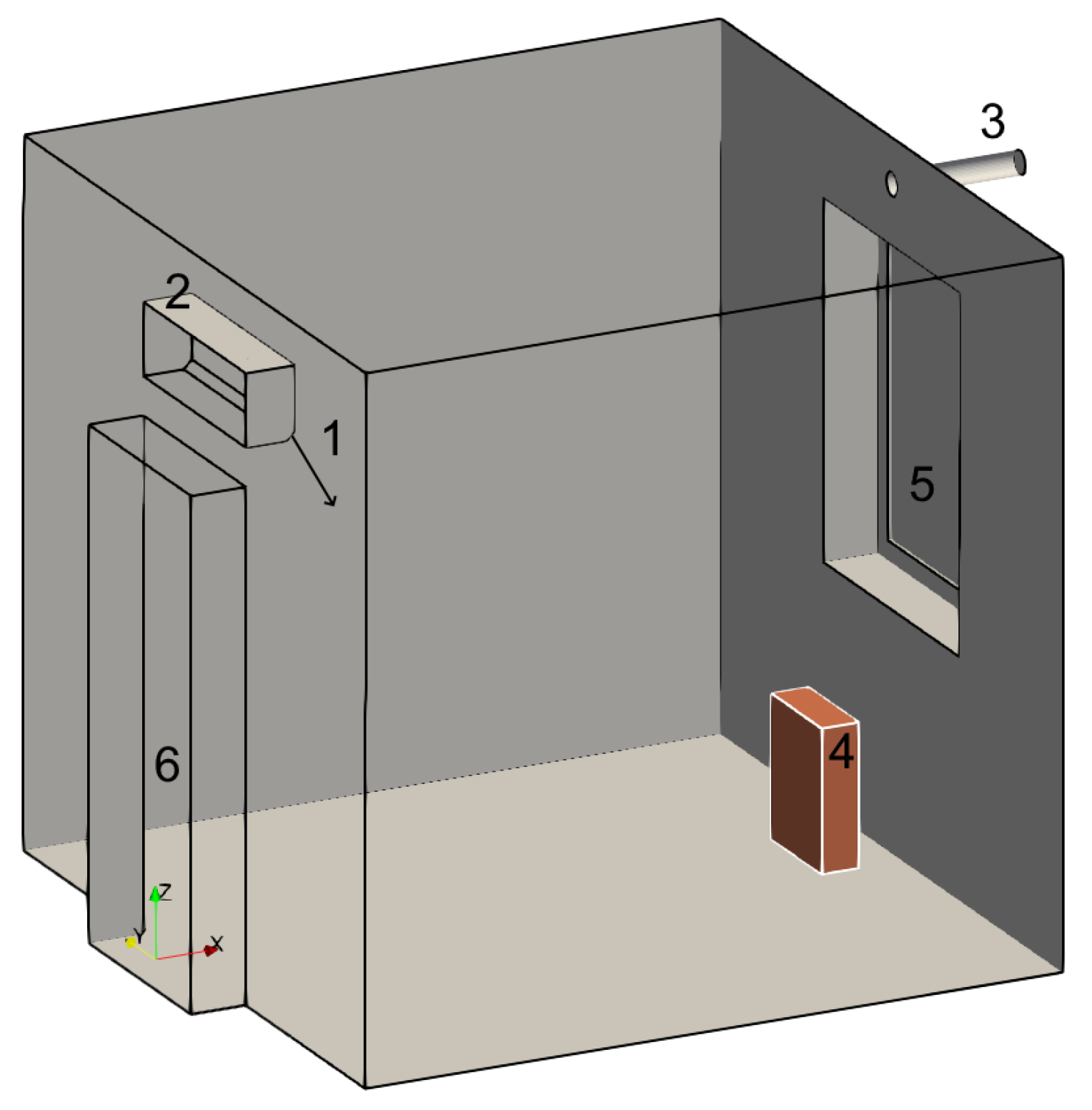
2.2. Experimental Setup
3. Results and Discussion
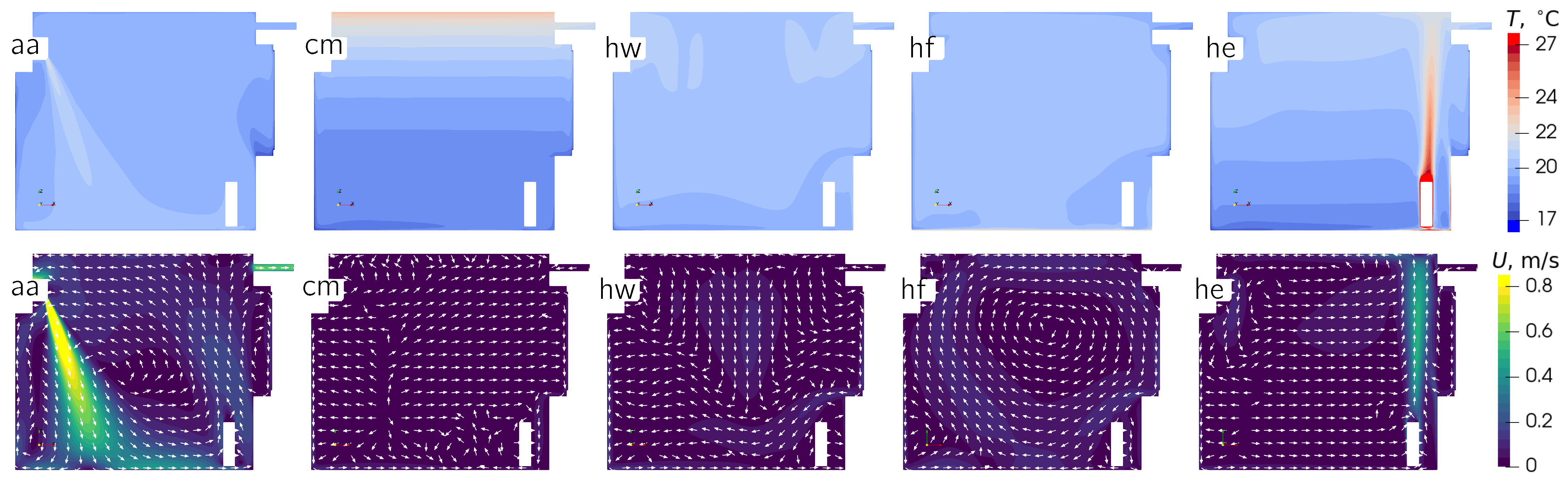
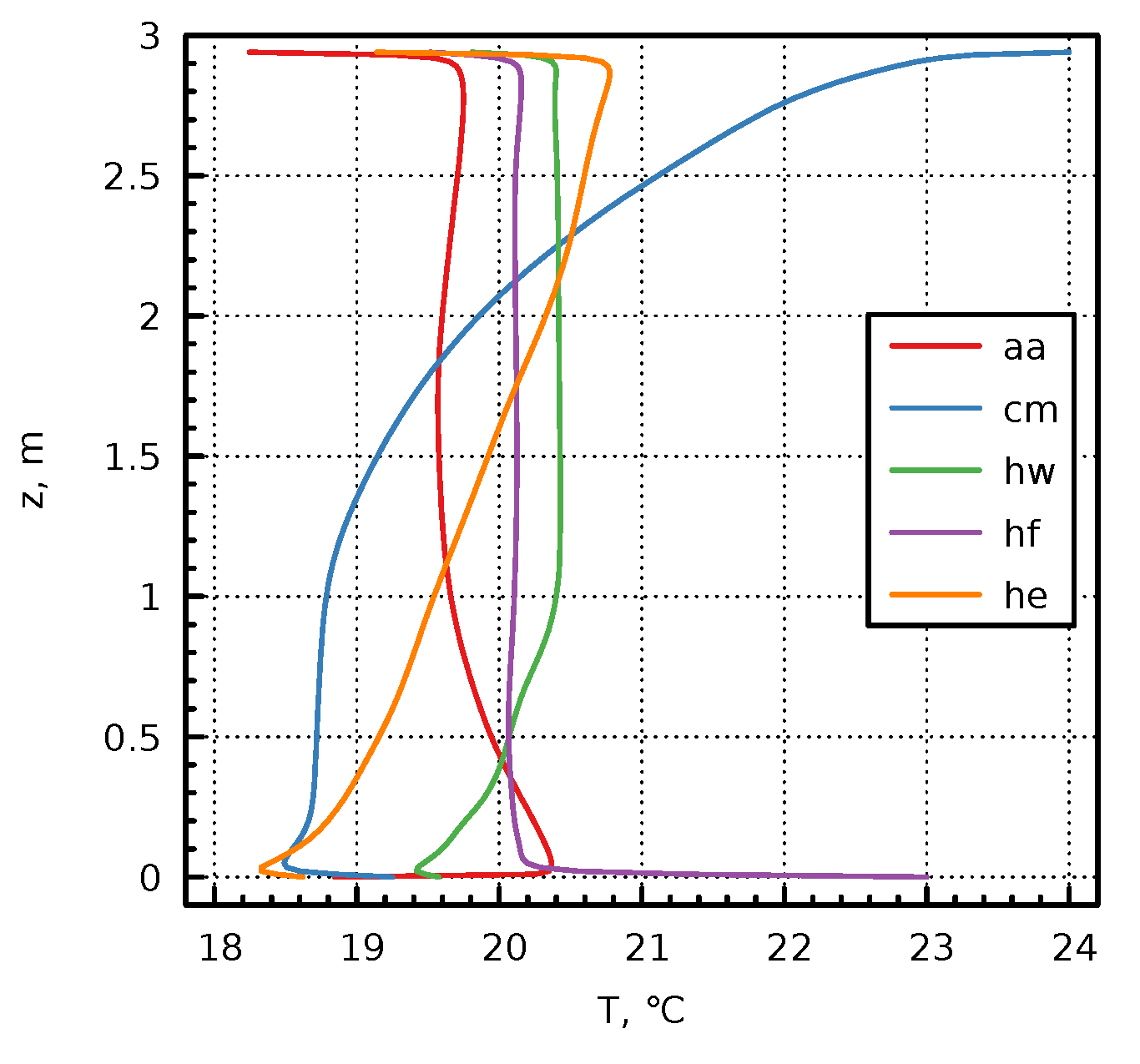
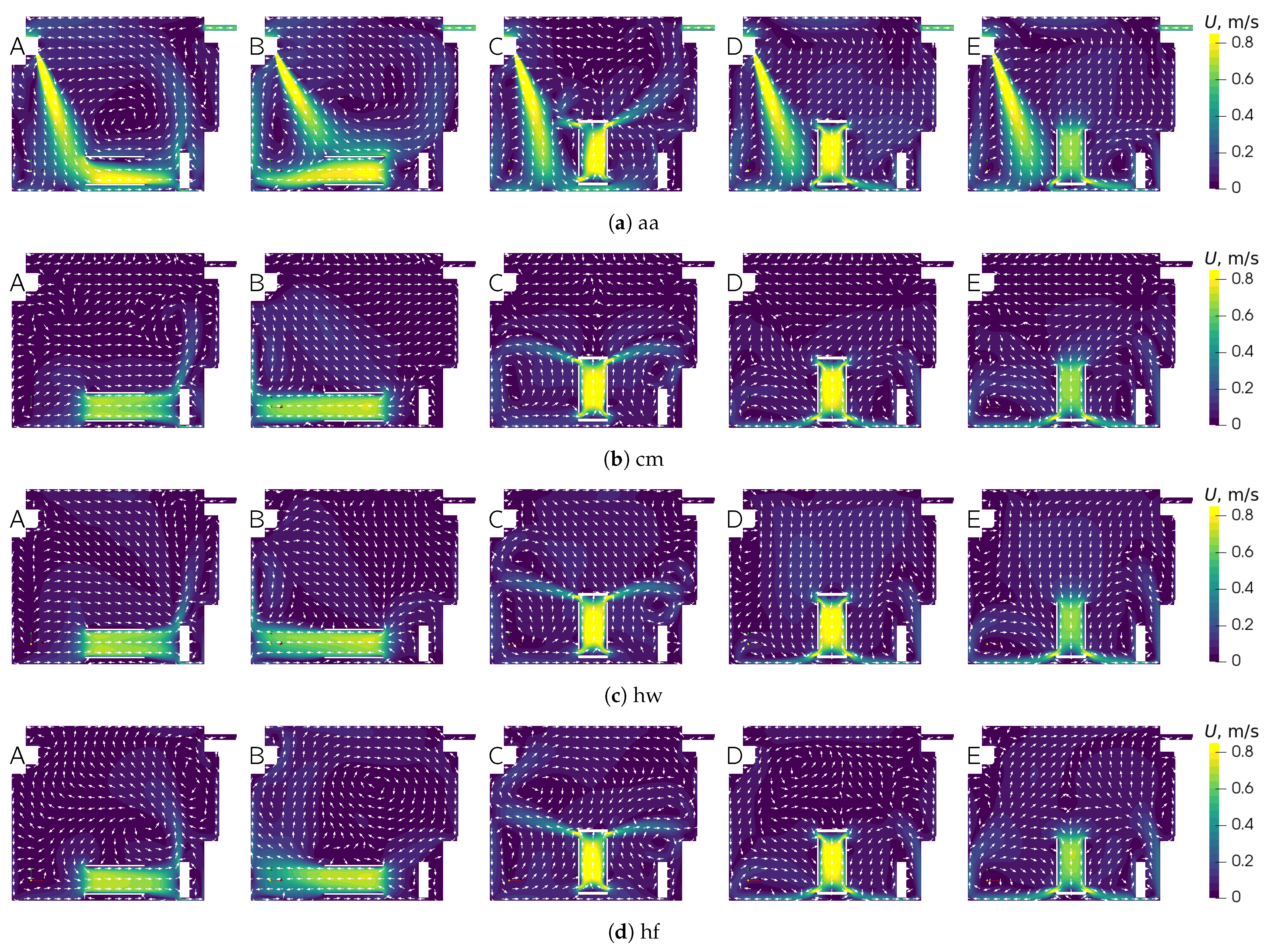
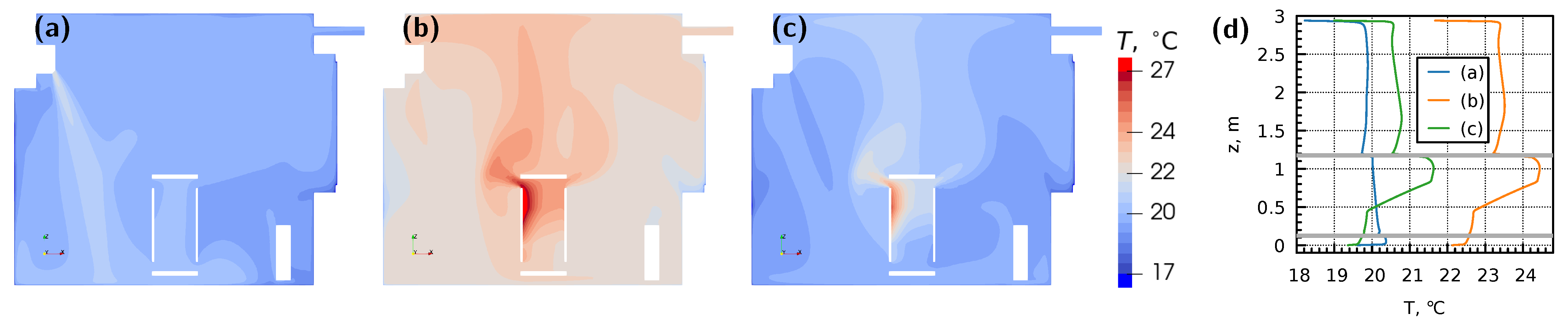
3.1. Numerical Results—Airflow
3.1.1. Without Air Cleaner
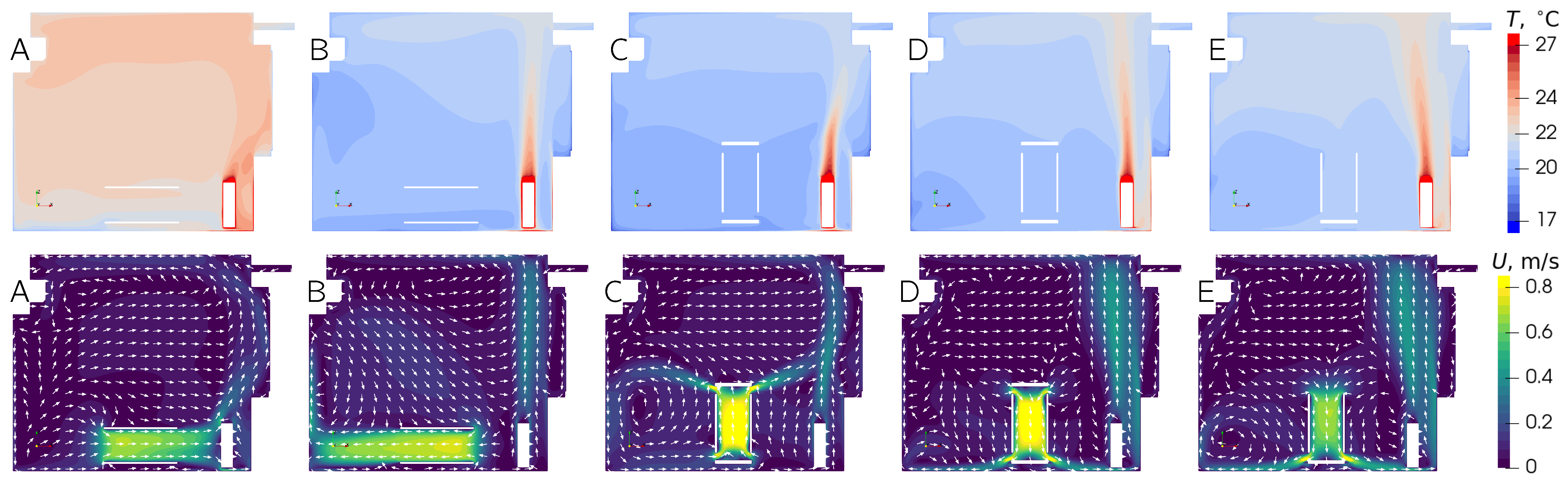
3.1.2. With Air Cleaner
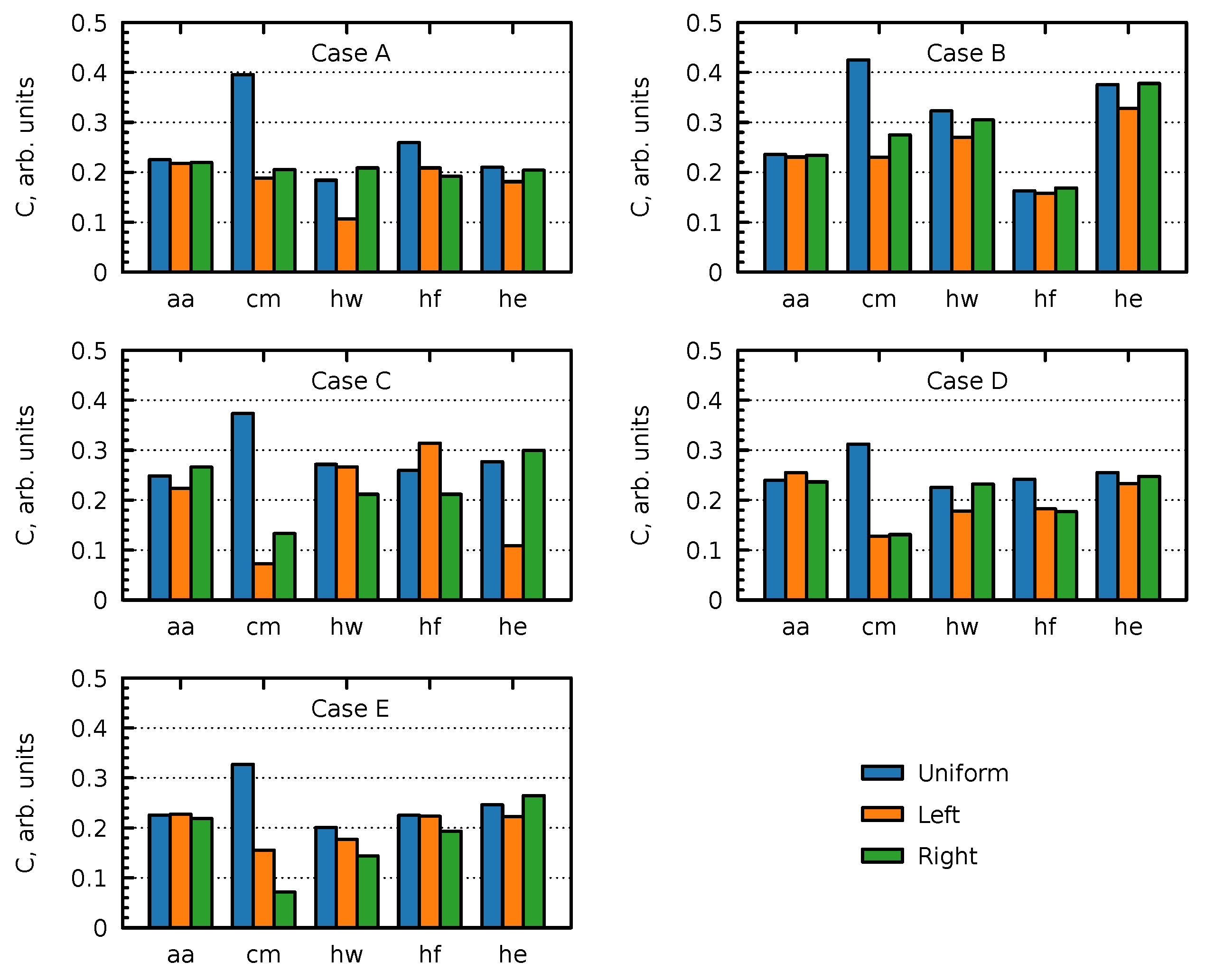
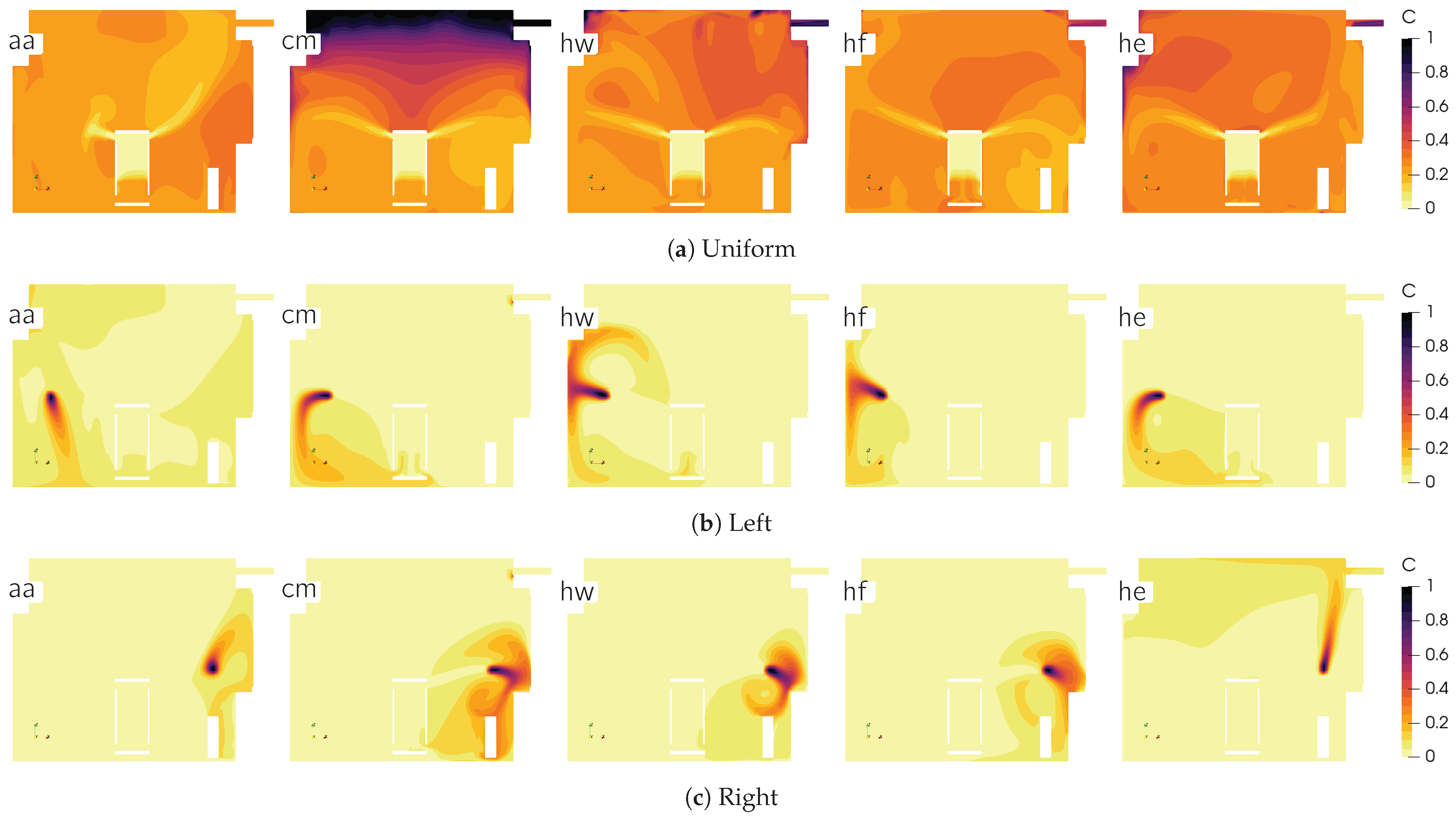
3.2. Numerical Results—Aerosol Transport
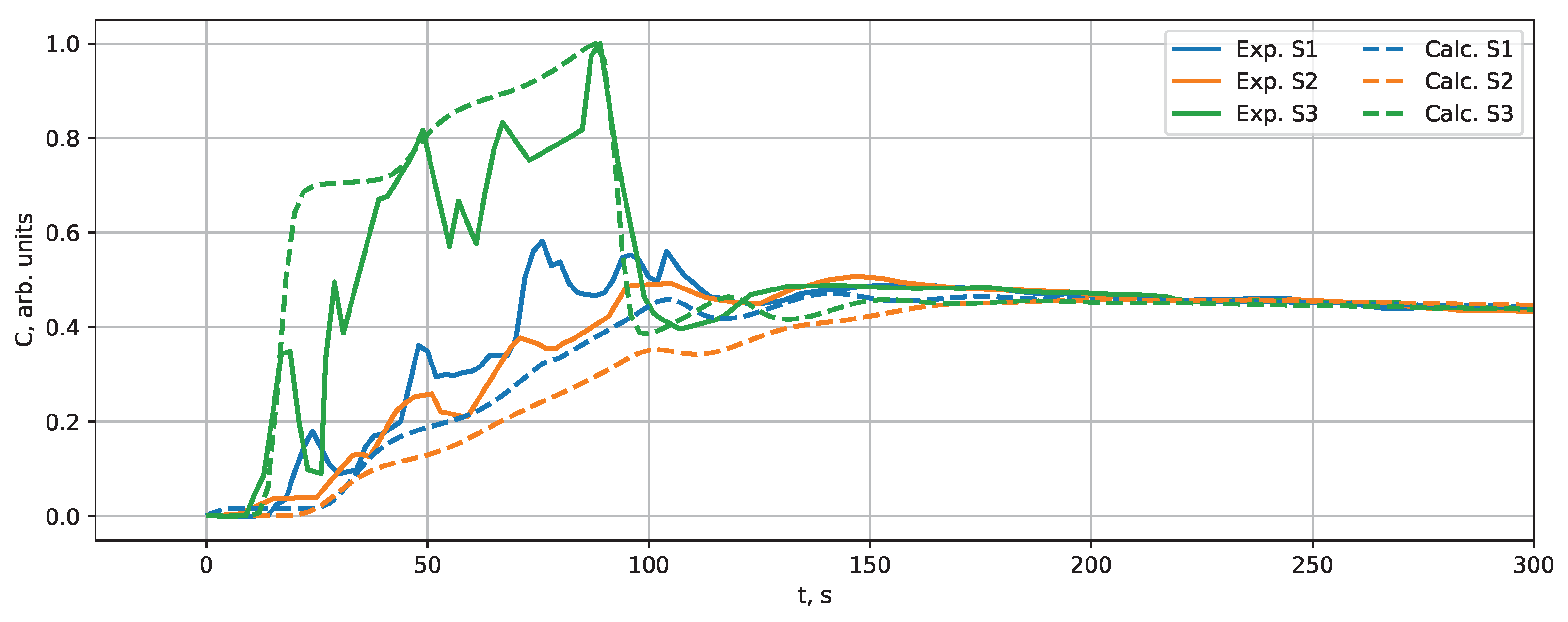
3.3. Experimental Results and Validation of Numerical Model
4. Summary and Conclusions
Author Contributions
Funding
Data Availability Statement
Conflicts of Interest
Abbreviations
| CADR | Clean air delivery rate |
| CFD | Computational fluid dynamics |
| HEPA | High-efficiency particulate air |
| PM | Particulate matter |
| PSM | Passive scalar model |
| RANS | Reynolds-averaged Navier–Stokes |
| UV | Ultraviolet |
| C | Normalized dimensionless mass concentration (arbitrary units) |
| Specific heat capacity | |
| D, , | Brownian, turbulent, and effective diffusion coefficient |
| Single-pass filtration efficiency | |
| k | Decay rate |
| Dynamic viscosity | |
| Kinematic viscosity | |
| P | Power |
| Pr, | Laminar and turbulent Prandtl number |
| Q | Volumetric flow rate |
| Re | Reynolds number |
| Density | |
| S | Source term for concentration |
| Sc, | Laminar and turbulent Schmidt number |
| t | Time |
| T | Temperature |
| Velocity | |
| V | Volume |
Appendix A


References
- Feng, Y.; Zhao, J.; Spinolo, M.; Lane, K.; Leung, D.; Marshall, D.; Mlinaric, P. Assessing the filtration effectiveness of a portable ultraviolet air cleaner on airborne SARS-CoV-2 laden droplets in a patient room: A numerical study. Aerosol Air Qual. Res. 2021, 21, 200608. [Google Scholar] [CrossRef]
- Mohamadi, F.; Fazeli, A. A review on applications of CFD modeling in COVID-19 pandemic. Arch. Comput. Methods Eng. 2022, 29, 3567–3586. [Google Scholar] [CrossRef] [PubMed]
- Rayegan, S.; Shu, C.; Berquist, J.; Jeon, J.; Zhou, L.G.; Wang, L.L.; Mbareche, H.; Tardif, P.; Ge, H. A review on indoor airborne transmission of COVID-19-modelling and mitigation approaches. J. Build. Eng. 2023, 64, 105599. [Google Scholar] [CrossRef]
- Tobisch, A.; Springsklee, L.; Schäfer, L.F.; Sussmann, N.; Lehmann, M.J.; Weis, F.; Zöllner, R.; Niessner, J. Reducing indoor particle exposure using mobile air purifiers—Experimental and numerical analysis. AIP Adv. 2021, 11, 125114. [Google Scholar] [CrossRef]
- Burgmann, S.; Janoske, U. Transmission and reduction of aerosols in classrooms using air purifier systems. Phys. Fluids 2021, 33, 033321. [Google Scholar] [CrossRef]
- Curtius, J.; Granzin, M.; Schrod, J. Testing mobile air purifiers in a school classroom: Reducing the airborne transmission risk for SARS-CoV-2. Aerosol Sci. Technol. 2021, 55, 586–599. [Google Scholar] [CrossRef]
- Küpper, M.; Asbach, C.; Schneiderwind, U.; Finger, H.; Spiegelhoff, D.; Schumacher, S. Testing of an indoor air cleaner for particulate pollutants under realistic conditions in an office room. Aerosol Air Qual. Res. 2019, 19, 1655–1665. [Google Scholar] [CrossRef]
- Srivastava, S.; Zhao, X.; Manay, A.; Chen, Q. Effective ventilation and air disinfection system for reducing coronavirus disease 2019 (COVID-19) infection risk in office buildings. Sustain. Cities Soc. 2021, 75, 103408. [Google Scholar] [CrossRef] [PubMed]
- Dbouk, T.; Roger, F.; Drikakis, D. Reducing indoor virus transmission using air purifiers. Phys. Fluids 2021, 33, 103301. [Google Scholar] [CrossRef]
- Qian, H.; Li, Y.; Sun, H.; Nielsen, P.V.; Huang, X.; Zheng, X. Particle removal efficiency of the portable HEPA air cleaner in a simulated hospital ward. Build. Simul. 2010, 3, 215–224. [Google Scholar] [CrossRef]
- Li, F.; Liu, J.; Ren, J.; Cao, X. Predicting contaminant dispersion using modified turbulent Schmidt numbers from different vortex structures. Build. Environ. 2018, 130, 120–127. [Google Scholar] [CrossRef] [PubMed]
- Abuhegazy, M.; Talaat, K.; Anderoglu, O.; Poroseva, S.V. Numerical investigation of aerosol transport in a classroom with relevance to COVID-19. Phys. Fluids 2020, 32, 103311. [Google Scholar] [CrossRef] [PubMed]
- Vuorinen, V.; Aarnio, M.; Alava, M.; Alopaeus, V.; Atanasova, N.; Auvinen, M.; Balasubramanian, N.; Bordbar, H.; Erästö, P.; Grande, R.; et al. Modelling aerosol transport and virus exposure with numerical simulations in relation to SARS-CoV-2 transmission by inhalation indoors. Saf. Sci. 2020, 130, 104866. [Google Scholar] [CrossRef]
- Foster, A.; Kinzel, M. Estimating COVID-19 exposure in a classroom setting: A comparison between mathematical and numerical models. Phys. Fluids 2021, 33, 021904. [Google Scholar] [CrossRef] [PubMed]
- Foat, T.G.; Higgins, B.; Abbs, C.; Maishman, T.; Coldrick, S.; Kelsey, A.; Ivings, M.J.; Parker, S.T.; Noakes, C.J. Modeling the effect of temperature and relative humidity on exposure to SARS-CoV-2 in a mechanically ventilated room. Indoor Air 2022, 32, e13146. [Google Scholar] [CrossRef]
- Liu, S.; Koupriyanov, M.; Paskaruk, D.; Fediuk, G.; Chen, Q. Investigation of airborne particle exposure in an office with mixing and displacement ventilation. Sustain. Cities Soc. 2022, 79, 103718. [Google Scholar] [CrossRef] [PubMed]
- Jain, A.; Duill, F.F.; Schulz, F.; Beyrau, F.; van Wachem, B. Numerical study on the impact of large air purifiers, physical distancing, and mask wearing in classrooms. Atmosphere 2023, 14, 716. [Google Scholar] [CrossRef]
- Dbouk, T.; Drikakis, D. On airborne virus transmission in elevators and confined spaces. Phys. Fluids 2021, 33, 011905. [Google Scholar] [CrossRef]
- Sen, N. Transmission and evaporation of cough droplets in an elevator: Numerical simulations of some possible scenarios. Phys. Fluids 2021, 33, 033311. [Google Scholar] [CrossRef]
- Foat, T.; Drodge, J.; Nally, J.; Parker, S. A relationship for the diffusion coefficient in eddy diffusion based indoor dispersion modelling. Build. Environ. 2020, 169, 106591. [Google Scholar] [CrossRef]
- Wang, M.; Lin, C.H.; Chen, Q. Advanced turbulence models for predicting particle transport in enclosed environments. Build. Environ. 2012, 47, 40–49. [Google Scholar] [CrossRef]
- Saidi, M.S.; Rismanian, M.; Monjezi, M.; Zendehbad, M.; Fatehiboroujeni, S. Comparison between Lagrangian and Eulerian approaches in predicting motion of micron-sized particles in laminar flows. Atmos. Environ. 2014, 89, 199–206. [Google Scholar] [CrossRef]
- Sajjadi, H.; Atashafrooz, M.; Delouei, A.A.; Wang, Y. The effect of indoor heating system location on particle deposition and convection heat transfer: DMRT-LBM. Comput. Math. Appl. 2021, 86, 90–105. [Google Scholar] [CrossRef]
- Sabanskis, A.; Vidulejs, D.D.; Teličko, J.; Virbulis, J.; Jakovičs, A. Experimental and numerical evaluation of the efficiency of an indoor air cleaner under different conditions. In Proceedings of the Healthy Buildings 2023 Europe, Aachen, Germany, 11–14 June 2023; pp. 522–530. [Google Scholar]
- OpenFOAM CFD Software. Available online: https://www.openfoam.com/ (accessed on 12 October 2023).
- Sabanskis, A.; Virbulis, J. Experimental and numerical analysis of air flow, heat transfer and thermal comfort in buildings with different heating systems. Latv. J. Phys. Tech. Sci. 2016, 53, 20–30. [Google Scholar] [CrossRef]
- Jakovics, A.; Gendelis, S.; Ratnieks, J.; Sakipova, S. Monitoring and modelling of energy efficiency for low energy testing houses in Latvian climate conditions. Int. J. Energy 2014, 8, 76–83. [Google Scholar]
- Virbulis, J.; Sjomkane, M.; Surovovs, M.; Jakovics, A. Numerical model for prediction of indoor COVID-19 infection risk based on sensor data. J. Phys. Conf. Ser. 2021, 2069, 012189. [Google Scholar] [CrossRef]
- Ounis, H.; Ahmadi, G. A comparison of Brownian and turbulent diffusion. Aerosol Sci. Technol. 1990, 13, 47–53. [Google Scholar] [CrossRef]
- Jiang, J.; Wang, X. On the numerical study of indoor particle dispersion and spatial distribution. Air Soil Water Res. 2012, 5, 23–40. [Google Scholar] [CrossRef]
- ANSI/AHAM AC-1; Method for Measuring Performance of Portable Household Electric Room Air Cleaners. Association of Home Appliance Manufacturers: Washington, DC, USA, 2006.


| Case | Explanation |
|---|---|
| aa | Air–air heat pump (air conditioner operating in heating mode) |
| cm | Capillary mat on the ceiling (heated ceiling) |
| hw | Capillary mat on the walls (heated walls) |
| hf | Heated floor |
| he | Radiator (heater) |
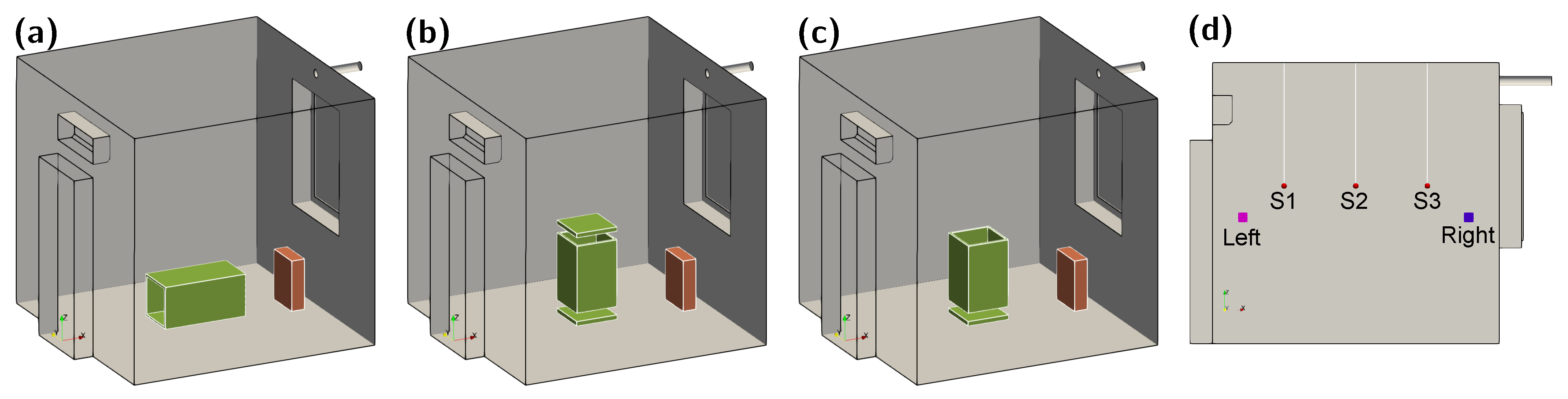
| Case | Explanation |
|---|---|
| A | Horizontal orientation, flow in direction (towards the radiator) |
| B | Horizontal orientation, flow in direction (towards the door) |
| C | Vertical orientation, flow in direction (upwards) |
| D | Vertical orientation, flow in direction (downwards) |
| E | Vertical orientation, top lid removed, flow in direction (downwards) |
| Case | , °C | , W | , °C |
|---|---|---|---|
| aa | 22 | 335 | 19.7 |
| cm | 24 | 223 | 19.6 |
| hw | 21 | 135 | 20.3 |
| hf | 23 | 222 | 20.1 |
| he | 49 | 246 | 19.9 |
| Sensor | Left | Right | ||
|---|---|---|---|---|
| Exp. | Calc. | Exp. | Calc. | |
| S1 | 37.6 | 37.4 | 34.6 | 36.1 |
| S2 | 36.7 | 35.7 | 35.4 | 35.3 |
| S3 | 35.7 | 36.9 | 36.7 | 35.3 |
Disclaimer/Publisher’s Note: The statements, opinions and data contained in all publications are solely those of the individual author(s) and contributor(s) and not of MDPI and/or the editor(s). MDPI and/or the editor(s) disclaim responsibility for any injury to people or property resulting from any ideas, methods, instructions or products referred to in the content. |
© 2023 by the authors. Licensee MDPI, Basel, Switzerland. This article is an open access article distributed under the terms and conditions of the Creative Commons Attribution (CC BY) license (https://creativecommons.org/licenses/by/4.0/).
Share and Cite
Sabanskis, A.; Vidulejs, D.D.; Teličko, J.; Virbulis, J.; Jakovičs, A. Numerical Evaluation of the Efficiency of an Indoor Air Cleaner under Different Heating Conditions. Atmosphere 2023, 14, 1706. https://doi.org/10.3390/atmos14121706
Sabanskis A, Vidulejs DD, Teličko J, Virbulis J, Jakovičs A. Numerical Evaluation of the Efficiency of an Indoor Air Cleaner under Different Heating Conditions. Atmosphere. 2023; 14(12):1706. https://doi.org/10.3390/atmos14121706
Chicago/Turabian StyleSabanskis, Andrejs, Dagis Daniels Vidulejs, Jevgēnijs Teličko, Jānis Virbulis, and Andris Jakovičs. 2023. "Numerical Evaluation of the Efficiency of an Indoor Air Cleaner under Different Heating Conditions" Atmosphere 14, no. 12: 1706. https://doi.org/10.3390/atmos14121706