Article

Assessment of Urban Local High-Temperature Disaster Risk and the Spatially Heterogeneous Impacts of Blue-Green Space

1
College of Horticulture and Landscape Architecture, Northeast Agricultural University, Harbin 150030, China
2
Zhejiang Province Institute of Architectural Design and Research, Hangzhou 310056, China
*
Author to whom correspondence should be addressed.
Atmosphere 2023, 14(11), 1652; https://doi.org/10.3390/atmos14111652
Submission received: 22 September 2023 / Revised: 27 October 2023 / Accepted: 30 October 2023 / Published: 3 November 2023

Abstract

:
Urban high-temperature disasters have gradually emerged as a significant threat to human society. Therefore, it is crucial to assess and identify areas at risk of such disasters and implement urban planning measures aimed at mitigating their impact. Additionally, a multitude of studies have demonstrated the significant cooling effect of urban blue-green spaces (UGBS), which play a pivotal role in urban environments. Incorporating a UBGS layout into planning and evaluation processes has substantial potential for mitigating high-temperature disasters. This paper presents the construction of a set of assessment processes for mitigating urban high-temperature disaster risk using a UBGS structure layout specifically for the main urban area of Harbin, China. We employed GIS and multi-source remote sensing imagery to develop local climate zone (LCZ) maps applicable to the designated study area. The differentiated impact of UBGS factors on high-temperature disaster risk was determined using the multi-scale geographical weighted regression model (MGWR). The results showed the following: (a) There was an overall low risk level, with 19.61% of the high-risk areas concentrated within the second ring road, forming a spatial pattern characterized by “one line, one cluster”. (b) The risk of the building category LCZs was generally higher than that of the natural category LCZs. The risk of the architectural LCZs could be summarized as the risk of low-density LCZs being smaller than that of the high-density LCZs, except LCZ 5. The mean value of the LCZ 2 and LCZ 5 types was the highest. (c) Through indicator screening, AREA_MN, SHAPE_MN, PD, and NP were found to be significant determinants influencing the risk, and the effectiveness and spatial differentiation of these main factors exhibited notable disparities. (d) By comparing different LCZ types, we concluded that the mitigation effect of these factors on risk may be interfered with by building height (BH); NP may be positively interfered with by BH; and PD and SHAPE_MN may be negatively interfered with by BH. The research results provided a new perspective and practical scientific basis for high-temperature disaster risk-mitigation planning based on UBGSs under LCZ classification.

1. Introduction

China’s urbanization rate has reached 65.22% since urbanization became a key growth strategy [1,2]. However, rapid economic growth brought on by urbanization has also resulted in the original natural landscape being replaced by roads and buildings, which has contributed to frequent extreme heat in cities under the dual influence of low ground permeability and global warming [3,4]. The frequency change of extreme weather will have a profound impact on human society and the natural environment [5]. As a typical urban climate problem, high-temperature disasters brought on by extreme hot weather have become of concern to scholars in various fields [6,7]. In recent years, urban high-temperature disasters have led to a significant increase in morbidity and mortality. In 1995, the Chicago high-temperature disaster caused more than 700 deaths in one week [8]. In 2010, the heat disaster in New Delhi put more than 100 million people at risk from heat waves. In 2023, a deadly heat wave called “Cerberus” swept across Europe, with temperatures in Italy reaching a staggering 48.8 degrees Celsius. The risk assessment of urban high-temperature disasters has become an important topic in the study of climate change due to the increasingly frequent occurrence of extreme high-temperature events. To support the sustainability of urban development, a thorough investigation of the relationship between urban landscape characteristics and high-temperature disaster risks is crucial.
The study of high-temperature-disaster risk assessment has grown together with the growth of natural-disaster risk assessment. In order to address the hazards of climate change, the IPCC’s fifth report recommended a framework for assessing the risk of natural disasters based on the notion of “disaster stress-social vulnerability exposure” [9]. In this approach, the three characteristics of disaster factors, disaster environments, and disaster-carrying bodies are used to underline the significance of the entire process of climatic disaster occurrence. This approach has been widely used in the investigation of high-temperature-disaster risk assessment. By merging GIS and remote sensing pictures in San Diego, Inostroza et al. created a high-temperature risk-assessment model based on exposure, sensitivity, and adaptability [10]. Thanvisitth-pon developed an urban high-temperature risk-assessment framework using the four dimensions of risk, exposure, sensitivity, and adaptive capability, while also assessing the urban high-temperature risk in Bangkok, Thailand [11]. Some of these studies have conducted in-depth investigations into the spatial and temporal distribution of high-temperature disaster risk, proving that there is a spatial and temporal dynamic change of high-temperature disaster risk [12]. Yin used daily meteorological monitoring data from 1989 to 2018 to explore the spatial and temporal distribution pattern of high-temperature disaster risk in the Belt and Road region [13]. The research on high-temperature catastrophe risk in the literature, however, has primarily focused on analyzing the risk level in a particular study region, and the research findings have been focused on creating each study area’s risk map [14,15]. The quantitative role of the driving factors affecting high-temperature disaster risk remains uncertain [16]. The presence of uncertainty is a constraint on the capacity of planners to provide precise suggestions about the optimization of land use. Additionally, it restricts the potential of landscape design to mitigate urban heat issues [17,18].
In order to explore the elements relevant to mitigating heat disasters, researchers in various fields have studied various urban cooling measures, including the use of cooling materials and colors [19,20], as well as the planning of urban blue-green spaces (UBGSs) [21]. Numerous studies have demonstrated that UBGSs may greatly reduce urban heat, lower surface temperatures, and be more cost-effective [22,23]. Green spaces (including forests, urban parks, green roofs, and other vegetated areas) can cool the air through evaporation and also reduce the ground temperature by reducing the solar radiation directly reaching the ground through shade [24]. Blue spaces (including water-covered areas such as rivers, lakes, artificial water features, etc.) offer great cooling capacity due to their high thermal capacity (i.e., they heat up more slowly than air and other substances for the same amount of solar radiation) and evaporation and convection processes [25,26]. Studies have also shown that UBGS cooling is controlled by environmental factors such as building height/density [27,28]. However, high-temperature hazard risk depends not only on the thermal hazard caused by excessively high temperatures but also on sensitivity and vulnerability [10,11]. Additionally, UBGSs may enhance residents’ participation in outside activities, increasing the risk of residents suffering heat-related injuries [29]. Most studies in the existing literature have concentrated on the direct relationship between landscape pattern indicators, such as size, shape, type, density, connectivity, and complexity (composition and configuration) of UBGSs and land surface temperature [30,31,32,33], but there has been less focus on the trade-off between these indicators and the risk of high-temperature disasters. It is unclear whether enhancing UBGSs will reduce the likelihood of high-temperature disasters, and further research is required to determine the full impact of UBGS landscape patterns on this risk.
Due to limitations in the domains of researchers and planners, in past urban climate studies, only a small proportion of the explanations of the effects of urban landscape elements on the climate have been successfully translated into planning practices [34,35,36]. Weather researchers are unfamiliar with planning needs at all scales, and planners struggle to understand the complex interactions between the climate and cities. A landscape classification framework with a high degree of visualization that is simple to understand and apply is required to bridge the knowledge gap between various fields and aid in the translation of research findings on high-temperature disaster risk into sustainable urban planning strategies. In order to clearly distinguish between the urban landscape and urban climate, this study divided cities into local climate zones (LCZs) [37] and examined the effect of UBGS landscape patterns on the risk of high-temperature disasters under the LCZ scheme. The LCZs were divided into two categories. There were 17 LCZ types, including 10 building category LCZs (LCZs 1–10) and 7 natural category LCZs (LCZs A–G). The LCZ scheme has been successfully applied to many urban high-temperature problems [38,39], but few researchers have used it in the risk assessment of high-temperature disasters. Existing studies have highlighted the importance of 3D and 2D features in urban environments in ameliorating extreme heat events [40], while studies have also demonstrated differences in climate characteristics among different building class LCZs [41]. Therefore, it is of great significance to explore the distribution of local high-temperature disaster risks and to thoroughly study the impact of UBGSs on high-temperature disasters. However, most current studies have used fixed grids to divide basic units, which not only has poor accuracy but also does not provide effective support for field environment optimization. Based on current research, this paper focused on three targets: (1) carrying out a more thorough LCZ categorization in the study region; (2) creating a model for assessing the risk of high-temperature disasters, assessing high-temperature disasters from the angles of risk of disaster-causing danger, disaster-generating sensitivity, and disaster-bearing vulnerability, and determining the distribution of high-temperature disaster risk; and (3) using MGWR to identify UBGS landscape pattern factors that can be used to regulate the risk of high-temperature disasters. The research results provide a reference for mitigating urban high-temperature disasters and the rational planning of urban land use.

2. Materials and Methods

2.1. Study Area

Harbin (latitude 45°38′19″–45°51′47″ N, longitude 126°28′31″–126°50′7″ E) is located in the south of Heilongjiang Province, with a total area of about 53,100 square hectares. It is in the temperate zone as a whole, with a temperate continental monsoon climate and obvious monsoon characteristics, four distinct seasons, and large temperature differences throughout the year. The lowest temperature exceeds minus 40 °C, the highest temperature can reach 39.2 °C, and the average annual precipitation is 649 mm. As a typical old industrial city, Harbin’s rapid urbanization has caused a series of problems, such as habitat fragmentation and environmental pollution. According to the statistics of the Heilongjiang Meteorological Bureau, in the most recent 10 years, the maximum temperature in summer in the city has gradually increased, the number of high-temperature days has gradually increased, and the disasters caused by high temperatures in the city have gradually increasingly affected the daily life of residents. This study took the main urban area of Harbin as the research area, and the research scope was consistent with the boundary of the outer ring of Harbin, which is composed of the central urban area surrounded by high-speed roads (as shown in Figure 1).

2.2. Overall Workflow

To evaluate the danger of the urban area experiencing a high-temperature disaster and investigate the impact of UBGSs on its geographical heterogeneity, first, we merged building data with RS data to identify the LCZs as the research scale. Based on this, we undertook a thorough assessment of disaster-causing danger, disaster-generating sensitivity, and disaster-bearing vulnerability, and determined the distribution of urban high-temperature disaster risk using RS data and GIS. Secondly, we created a regression model using high-temperature disaster risk as the dependent variable, and we filtered the UBGS landscape pattern index computed from LULC data as an independent variable. We assessed the performance of the OLS, GWR, and MGWR by comparing the sizes of R2 and AICc. Finally, the important UBGS landscape pattern characteristics that could be utilized to control the danger of an urban high-temperature disaster risk were identified, and the spatial factors were incorporated into the high-temperature disaster risk-mitigation approach. The main workflow of this article is shown in Figure 2.

2.3. Data

The RS image data used in this study (Table 1) included Sentinel-2A remote sensing images and Landsat 8 remote sensing images, which were used for land-use analysis and land-surface-temperature inversion, respectively. Basic geographic information data (Table 2), including building, road network, POI, and population data, were used for LCZ classification and high-temperature-disaster risk assessment.

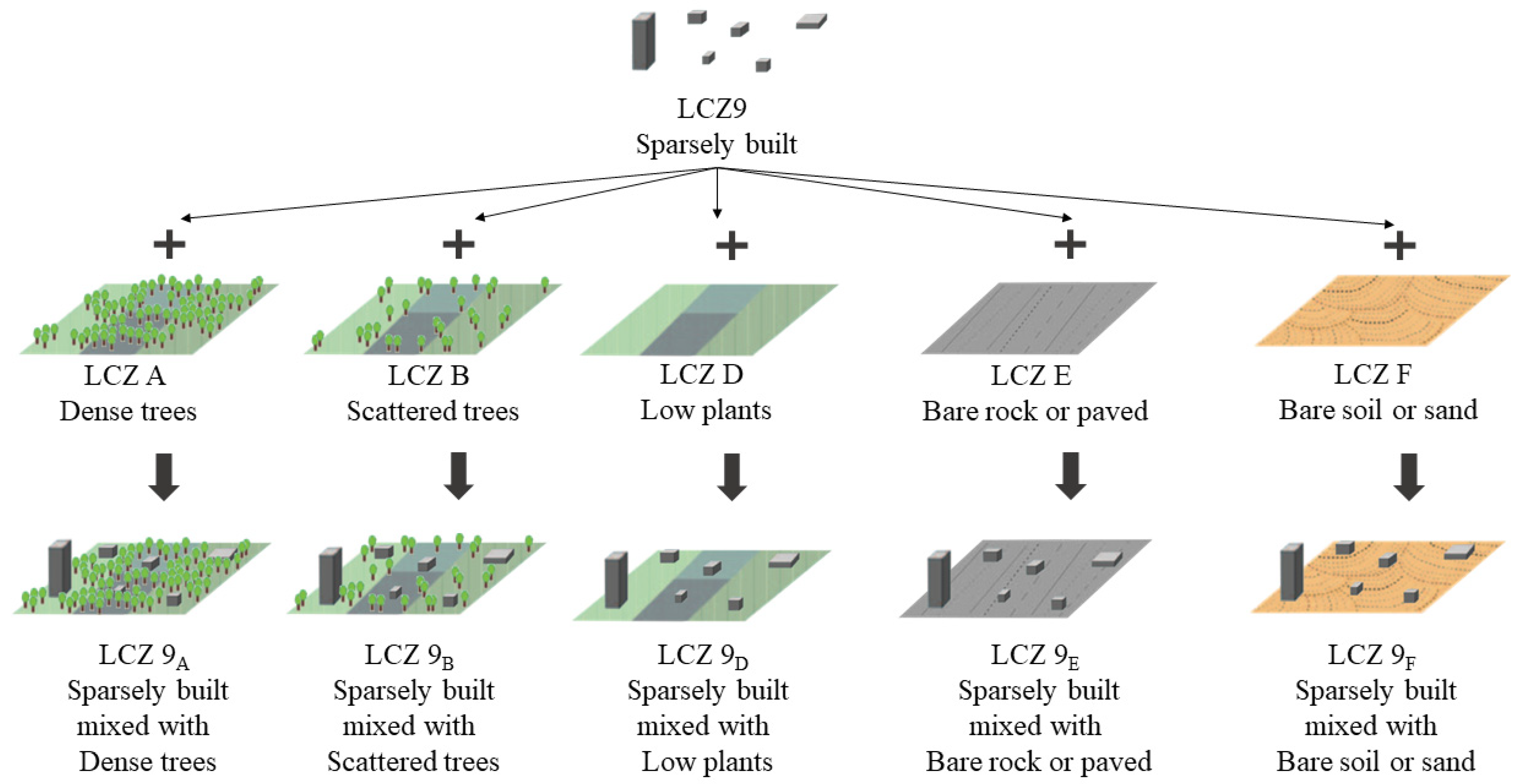
2.4. LCZ Classification

The urban architectural form affects the urban climate [42]. The LCZ system systematically classifies complex urban spaces from the perspective of climate effects, connecting “urban structure” and “urban climate elements”. Stewart and Oke divided the entire LCZ system into building category LCZs and natural category LCZs [37]. Therefore, based on the natural conditions of the central urban area in Harbin city, relevant indicators were calculated to classify the building category LCZs [43]. The calculation formula is shown in Appendix A. Additionally, the dominant land-cover type divided by the land-use data served as the foundation for the classification of the natural category LCZs. Finally, we combined the building category LCZs and the natural category LCZs based on the actual conditions in the study region [44] to obtain the final LCZ classification (Table 3). To reflect the building types between LCZ 9 and the natural environment classification, LCZ 9 was subdivided into five subclasses, as illustrated in Figure 3.

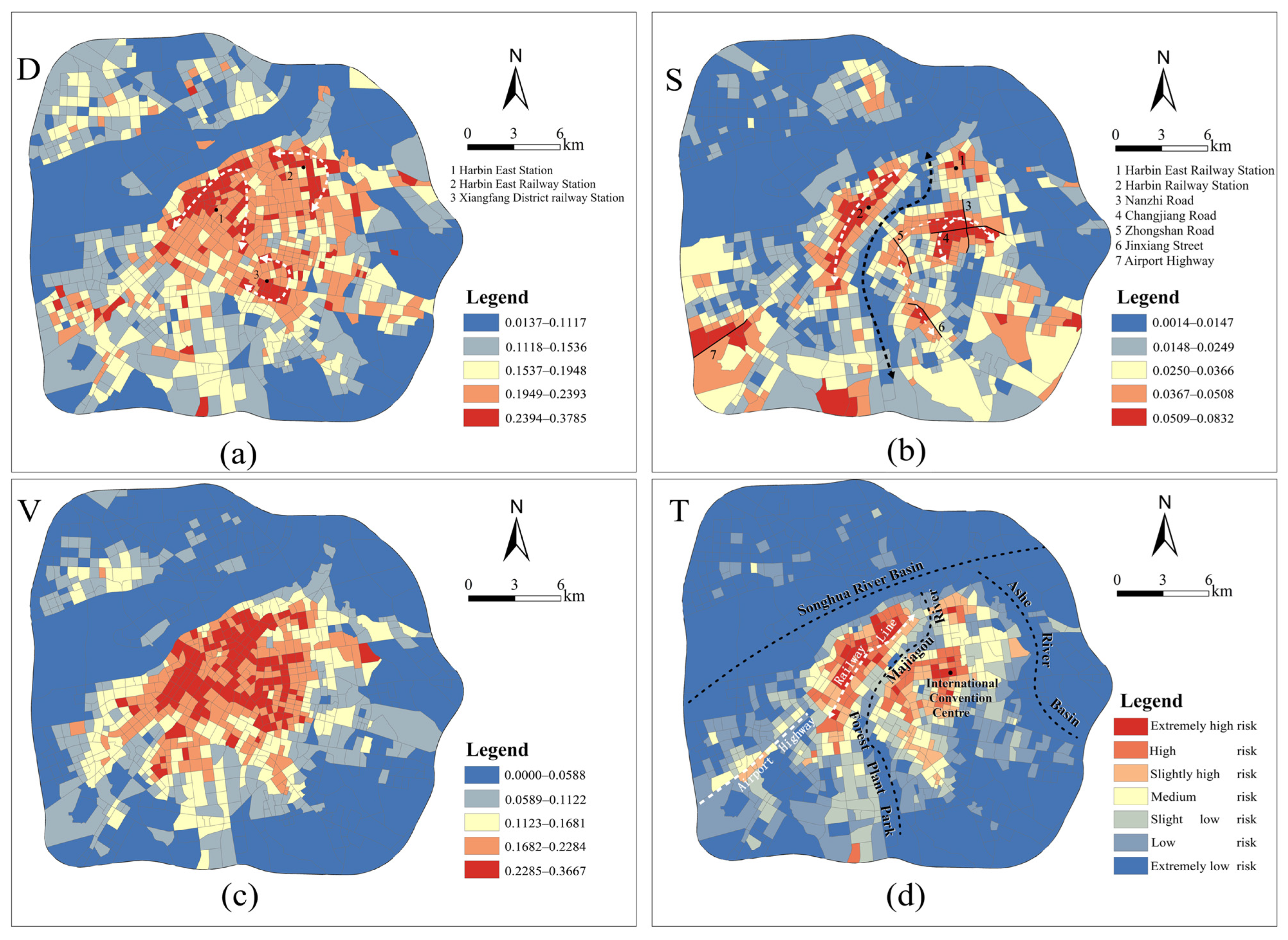
2.5. High-Temperature-Disaster Risk Assessment

In this study, a framework for assessing urban high-temperature disaster risk (T) was developed. The risk was divided into three categories: danger of disaster generation (D), sensitivity to disaster generation (S), and vulnerability to disaster bearing (V).

2.5.1. D Factors

The D factors were the factors that induced the formation of T. Based on previous studies, we chose surface temperature and urban development intensity as hazard assessment indicators [45]. In order to determine the surface temperature, we employed RS data for surface temperature inversion. We then used building data to determine the level of urban development, which included BSF and the normalized building index (NDBI). The NDBI can represent the proportion of impervious surfaces and is an important indicator of the urbanization level. The smaller the NDBI, the smaller the urban building land area, that is, the smaller the proportion of impervious surfaces. In this study, Landsat 8 data with 30 m resolution were used to calculate the NDBI. The calculation formula is shown in Appendix B.

2.5.2. S Factors

The natural environment dominates the S factors created by T. The primary natural environmental element, according to earlier studies, is water permeability, which includes river systems and forest vegetation [46]. As a result, the basic research unit’s distance from water and vegetation coverage (FVC) was chosen as the evaluation indices of disaster environmental sensitivity. The research shows that the higher the vegetation coverage and the shorter the distance to water, the better the cooling effect [21]. Therefore, considering that FVC and proximity to water are negative indicators, the reciprocal value of the above indicators was considered in the sensitivity evaluation. In this study, we used ArcGIS to determine the proximity to water and Landsat 8 remote sensing image data to calculate the FVC. The calculation formula is shown in Appendix B.

2.5.3. V Factors

Urban areas with a high population density and economic agglomeration are particularly vulnerable to the threat of high temperatures and are more likely to experience unfavorable side effects that exacerbate the harm caused by T [47]. Children and the elderly are particularly susceptible to heat disasters [48]. Therefore, population density (PD) and facility density were selected as V evaluation indicators in this study, in which population density included population density under 15 years old and population density over 60 years old, and facility density included living facility density and production facility density. In this study, demographic data and POI data were used to calculate the PD and facility density.

2.5.4. T Methods

(1)
Calculation of the T index
According to previous studies, the multiplication and division of indicators are more effective than addition and subtraction in reflecting the synergistic relationship between indicators [49]. Therefore, the T model of this study was as follows.
F D R I = D × S × V
In the formula, FDRI represents the T index, and the larger the value, the higher the risk degree; D represents the disaster-causing danger; S represents the disaster-generating sensitivity; and V represents the disaster-bearing vulnerability.
According to the corresponding weights, the comprehensive indexes of D, S, and V were calculated [49]. The formula was as follows:
D j = i = 1 m X i j × w j
where Dj is the comprehensive risk index of unit j, m is the number of indicators, Xij is the range normalization value of index j of unit i, and wj is the weight of index j. The sensitivity composite index Sj and the vulnerability composite index Vj were calculated by the same method.
(2)
Determination of the weight of each influencing factor
There are two types of index-weight calculation techniques: subjective weighting methods and objective weighting methods. The expertise of relevant academics can be used in the subjective weighing approach; however, the weight will be unstable because it is based on the evaluator’s own preferences. The objective weighing method fixes the problem of data stability, but the outcome can still be readily erroneous in terms of relevance. In order to determine the weights of each index, this study used both a subjective weighting method and an objective weighting method [50].
This study employed the analytic hierarchy process (AHP) as a subjective weighting method to assess the importance of indicators associated with high-temperature disasters. Initially, an analytic hierarchy model was constructed, consisting of a target layer, a criterion layer, and an indicator layer. Subsequently, expert scoring was utilized to determine the scores for each factor, and the judgment matrix was employed to derive the index weights for each level. These weights were then utilized as the subjective weights for this study.
When weighing indications for high-temperature disasters, the entropy technique was utilized as an objective method. To determine the objective weight of this study, the extreme value approach was utilized first for standardization, and the entropy method was used for thorough evaluation based on each indication standardization stage.
Table 4 displays the final weight of each index, which was determined by the weighting and averaging 70% of the subjective weight findings and 30% of the objective weight results.

2.6. Analysis of the Influence of the UBGS Landscape Pattern on T

The landscape pattern index can consolidate a lot of information on landscape patterns and show how they fit together structurally and in space [30]. With “optimized stock” planning, the cooling effect cannot be obtained by increasing UBGSs over a large area [51]. Therefore, it is very important to study how the size, form, and combination of UBGSs affect T. This will allow us to find the best way to use space to fully take advantage of the cooling effect of UBGSs. We used T as the dependent variable and calculated the number of patches (NP), patch density (PD), average patch area (AREA_MN), and average shape index (SHAPE_MN) as independent variables [30,31,32,33] (see Appendix C for a list of indicators and how to calculate them). This allowed us to find the regulatory factors by which UBGSs influence T intensity.
As a variation of the standard geographically weighted regression (GWR) model, multi-group geographically weighted regression (MGWR) is a good local regression method that can solve and explain spatial heterogeneity [52,53]. At runtime, each independent variable is given its own appropriate bandwidth. The bandwidth of the variable can show the size of the variable’s spatial effect on the dependent variable, and the spatial process model built using the multi-bandwidth method is more accurate [54,55]. This study explored the effects of multiple UBGS landscape pattern indicators on high-temperature hazard risk; the use of MGWR made the results more authentic. Before using the multi-scale geographically weighted regression model (MGWR), we used the multiple linear stepwise regression method to remove variables that were too similar. Then, MGWR was used to find the different regulatory factors that were linked to the T.
y i = j = i k β b w j ( u i , v i ) x i j + ε i
here, yi represents the observation value of the dependent variable at the ith sample point; βbwj (ui, vi) is the regression coefficient of the jth independent variable at the ith sample point; bwj is the differential bandwidth used by the regression coefficient of the jth variable; (ui, vi) represents the spatial coordinates of the ith sample point; xij is the observation value of the jth independent variable at the ith sample point; and εi is the stochastic perturbation term.
In order to verify the applicability of MGWR in this study, spatial autocorrelation analysis was carried out on the T index, and its spatial changes were visualized as spatial clusters with similar values. The results showed that the spatial distribution of the composite index had a strong positive spatial correlation. Units with a high-risk composite index were more likely to be adjacent to other units with a high-risk composite index (Appendix D). Therefore, the spatial heterogeneity of T in this study was verified, which supported the spatial characteristics of the data captured by the GWR program. In addition, the goodness of fit of R2, adjusted R2, and AICc were used as goodness-of-fit criteria to compare the performance of traditional OLS, classical GWR, and MGWR. Models that best fit the relationship between dependent and independent variables typically have higher adjusted R2, lower resists, and lower AICc [56,57].

3. Results

3.1. LCZ Classification Map

The research area was divided into 964 research units using the urban LCZ division approach, based on the fundamental unit of a road. To create the LCZ types, the height and density of buildings inside the basic unit were counted and coupled with land-use data.
Figure 4 depicts the LCZ map of the study area, as well as a few samples of classified images for the current LCZ classes. The LCZ map revealed a dispersion of the natural category LCZs in close proximity to the city center, whereas the building category LCZs were predominantly concentrated in the urban core (particularly evident in the yellow regions). Notably, 76.5% of LCZs fell under the construction category, while 23.5% belonged to the natural category, thus highlighting Harbin’s significant level of urbanization.
The two primary categories in the building district were LCZ 6 (open low-rise) and LCZ 5 (open midrise). The remaining space was dominated by LCZ 9B (sparsely built mixed with scattered trees) and LCZ 9E (sparsely built mixed with bare rock or paved). LCZ 2 and LCZ 3 (compact buildings) made up a total of 4.36% of the construction category for the LCZ. The majority of Harbin’s buildings are intermediate and low-rise, and the distribution is generally open.
Among the natural category LCZs, LCZ D (low plants) was the main landscape around the main urban area, followed by LCZ B (scattered trees) and LCZ E (bare rock or paved).

3.2. Assessment of Disaster Risk

3.2.1. D Factors

The average, maximum, and minimum values of D in Harbin were 0.1749, 0.3785, and 0.0137. The city was in medium danger overall. The numerical results were divided into five grades using the natural breakpoint method (Jenks). The value ranges, from small to large, were low danger risk (0.0137–0.1117), relatively low danger risk (0.1118–0.1536), medium danger risk (0.1537–0.1948), relatively high danger risk (0.1949–0.2393), and high danger risk (0.2394–0.3785).
Specifically, a total of 106 LCZs (11.00%) were in high-danger risk areas, and the high-danger risk areas were distributed in a “U” shape in the main urban area, widely distributed in the areas around the railway station and scattered along the airport expressway, Gongbin Road, and Xianfeng Road (Figure 5). There were 251 LCZs (26.03%) of relatively high-danger risk areas and 250 LCZs (25.93%) of medium-danger risk areas, which were radially interspersed with each other in the old city (inside the Second Ring Road) and along Xianfeng Road, Xuefu Road, and urban and rural roads. Outside the tricyclic ring, there were 357 LCZs (37.03%) with low danger risk, including low danger risk and relatively low danger risk.
As shown in Figure 6, LCZ2 and LCZ3 accounted for the highest ratio of 67% and 64%, respectively, in high-danger risk areas. Following this were LCZ 5, LCZ 6, and LCZ 4 at 20%, 19%, and 7%, respectively, showing that compact LCZs had a larger probability of disaster-causing danger than other LCZ types. In the relatively high-danger risk areas, LCZ 5 and LCZ 6 accounted for the highest ratios, at 54% and 48%, respectively, followed by LCZ 4, LCZ 9E, and LCZ 9F, at 30%, 27%, and 21%, respectively. LCZ 3 and LCZ E accounted for 15% and 14% of their own ratios, indicating that in the relatively high-danger risk areas, compact LCZs, open LCZs, and LCZs with a larger proportion of hard ground and bare soil were the most common.
It is important to note that the majority of LCZ 9E and LCZ 9F areas are in the construction phase and therefore have the potential to rise to high-danger risk areas. In contrast, most of the LCZ 9A, LCZ 9B, and LCZ 9D types were in low- or relatively low-risk classes, and the number of low-risk areas was LCZ 9D (20%) > LCZ 9A (19%) > LCZ 9B (2%). The proportion of vegetation cover in an LCZ unit may be an important factor in effectively resisting or reducing the risk of an LCZ disaster.

3.2.2. S Factors

The mean value, maximum value, and minimum value of S were 0.0257, 0.0832, and 0.0014. The numerical results were divided into five grades using the Jenks method. The value ranges, from small to large, were low sensitivity risk (0.0014–0.0147), relatively low sensitivity risk (0.0148–0.0249), medium sensitivity risk (0.0250–0.0366), relatively high sensitivity risk (0.0367–0.0508), and high sensitivity risk (0.0509–0.0832).
The number of LCZs with high or above-sensitivity risk was 228 (23.65%), and the number of LCZs with low or below-sensitivity risk was 539 (55.91%). In general, the sensitivity of the main urban area of Harbin was low risk. According to the spatial distribution of disaster-generating sensitivity, the high-sensitivity risk areas in the study area had the characteristics of “one belt, four cores”, with Harbin Railway Station as one belt and Haidong Railway Station, the intersection of Nanzhi Road and Changjiang Road, Jinxiang Street, and some sections of the airport road as the core. In addition, in the Jiangnan area, the LCZ containing Majiagou River was divided into the building category LCZs. The sensitivity values of the building category LCZs gradually moved toward the high-sensitivity risk core and decreased towards the main stream of the Songhua River or the Ashe River basin. The LCZ sensitivity values in the Jiangbei area were at a low-sensitivity risk or relatively low-sensitivity risk level.
As can be seen from Figure 6, LCZ 2 could not accurately characterize the characteristic rule of sensitivity grade proportion due to the small number of samples but could be summarized as a combination of the high-sensitivity type and medium-sensitivity type. The other building category LCZs had similar characteristics in terms of the proportion of sensitivity classes, among which the high sensitivity (including high sensitivity and relatively high sensitivity) of the LCZ 5 type accounted for the largest proportion, reaching 46%, followed by LCZ 6 and LCZ 3, at 34% and 31%, respectively. In these LCZ areas, vegetation was low, or the distance from the water was large, leading to a high sensitivity level. LCZ 9A and LCZ 9B generally had a high proportion of vegetation cover, so the low-sensitivity risk amount accounted for a relatively high proportion, at 88% and 77%, respectively. The natural category LCZs were mainly low-sensitivity risk types, in which the ratio of high sensitivity (including high sensitivity and relatively high sensitivity) of LCZ A accounted for 14%, which may have been due to the high proportion of vegetation in the dense forest area in the study area but the large distance from water.

3.2.3. V Factors

The average, maximum, and minimum values of V in Harbin City were 0.1255, 0.3667, and 0.0001, respectively. The numerical results were divided into five grades by the Jenks method. The value ranges, from small to large, were low vulnerability risk (0–0.0588), relatively low vulnerability risk (0.0589–0.1122), medium vulnerability risk (0.1133–0.1681), relatively high vulnerability risk (0.1682–0.2284), and high vulnerability risk (0.2285–0.3667).
Specifically, there were 117 (12.13%) LCZs in the high-vulnerability risk area and 199 (20.64%) LCZs in the relatively high-vulnerability risk area, as can be seen in Figure 5. In the Jiangnan area, the high-vulnerability risk area was widely distributed in the dense old urban area and interspersed with the relatively high-vulnerability risk area. The vulnerability value gradually decreased outside the city. In the Jiangbei region, most LCZ vulnerability levels were at medium risk or below.
As shown in Figure 6, high-vulnerability risk and relatively high-vulnerability risk areas were mainly concentrated in the building category LCZs, in which LCZ 4 and LCZ 5 accounted for the highest ratio, reaching 74% and 83%, followed by LCZ 6 and LCZ 9A, reaching 47% and 42%. In the study area, the open LCZ had a higher population density or facility density. The vulnerability value of LCZ 3 was relatively low, which may have been due to the constraints of low-rise building environments in this type of LCZ, resulting in a limited number of people and facilities, and its vulnerability value was smaller than that of the open LCZ.

3.2.4. T

In this study, the risk assessment model was used to comprehensively evaluate the study area in combination with D (weight 41.39%), S (weight 11.61%), and V (weight 47.01%). The numerical results were divided into seven grades by the Jenks method. The value ranges, from small to large, were extremely low risk (0–2.23 × 10⁻⁴), low risk (2.24 × 10⁻⁴–5.43 × 10⁻⁴), relatively low risk (5.44 × 10⁻⁴–9.40 × 10⁻⁴), medium risk (9.40 × 10⁻⁴–1.443 × 10⁻³), relatively high risk (1.444 × 10⁻³–2.106 × 10⁻³), high risk (2.107 × 10⁻³–2.979 × 10⁻³), and extremely high risk (2.980 × 10⁻³–5.324 × 10⁻³), to obtain T.
Overall, 189 (19.61%) LCZs were at medium risk or above. The study area was at low risk as a whole. As can be seen from Figure 5, the high-value comprehensive risk areas (graded above medium risk) in Jiangnan were distributed in a “one-line, one-cluster” pattern. The LCZ area along the railway of Harbin Station had a higher comprehensive risk, followed by the LCZ area centered on the Second Ring Road Exhibition Business District. The two risk areas were separated by the UBGS of the Majiagou River and the botanical gardens. They were also sandwiched between the Songhua River and the Ashe River basin. LCZ areas with UBGS facilities such as rivers and gardens had low comprehensive risk, followed by the suburbs outside the third ring road. It is worth noting that taking the LCZ along the airport road as an example, the LCZ along the road with the urban area as the core radiating outward also presented with higher risk.
As shown in Figure 6, the areas above the medium risk level were mainly concentrated in the building category LCZs. In addition to LCZ 2, LCZ 5 had the highest ratio of high risk (including relatively high risk, high risk, and very high risk), reaching 54%, while LCZ 3, LCZ 4, and LCZ 6 were all around 30%. Sparse building type LCZs (LCZ 9A-LCZ 9F) and natural category LCZs (LCZ A-G) had almost no high risk (including relatively high risk, high risk, and very high risk), except LCZ 9E, where high risk accounted for 18% of the ratio.

3.3. Regulatory Factors of T

Through linear stepwise regression, we screened 4 core independent variables from 16 UBGS landscape pattern indices, including NP, PD, AREA_MN, and SHAPE_MN (the linear regression results are given in Appendix E). The four indexes were used as independent variables to conduct regression analysis with T, and we explored their impact on T.
Table 5 lists the diagnosis results of the MGWR model. It can be seen that the goodness of fit of R2 of MGWR was higher than that of the classical GWR model, increasing from 0.829 for GWR to 0.870 for MGWR. The AICc value also decreased from 1600.141 for GWR to 1204.570 for MGWR. In general, MGWR had a better fitting degree, and the regression result was closer to the real level.
Figure 7 shows the MGWR model estimates for the relationship between T and UBGS factors. When the local coefficients of some variables are shown spatially, the local grid of variables that do not matter (p < 0.05) is colored white. In general, the UBGS landscape pattern has a large negative effect on T. The data showed that T can be reduced by increasing the number of UBGSs, increasing the density of UBGSs, increasing the area of UBGSs, and changing the shape of UBGSs. Specifically, the central and eastern areas to the south of the Songhua River, especially the NP in the northeast direction of the International Convention and Exhibition Center, had a significant negative impact on T. The negative coefficient of PD was mainly concentrated in the southern part of the study area along the Songhua River. The significant influence area of AREA_MN was very large, covering almost all the blocks on the south bank of the Songhua River. The negative coefficient of SHAPE_MN was concentrated in the area of North 14th Street along the Songhua River and near the Convention and Exhibition Center.
It can be seen from Figure 8 that in different types of LCZs, there is spatial heterogeneity in the influence of UBGSs on T. In LCZ 2 and LCZ 4, NP was a positive coefficient, indicating that blindly increasing the amount of UBGSs in LCZ 2 and LCZ 4 may have a counter-effect due to the excessive fragmentation of patches. In addition, by comparing the influence coefficients of UBGSs on T in each LCZ, it can be qualitatively concluded that the influence of NP, PD, and SHAPE_MN on T was affected by the BH in the unit. NP was positively affected by BH. The higher the BH, the stronger the negative influence of NP on T; PD and SHAPE_MN were negatively affected by building height, and the higher the BH, the weaker the negative influence of PD and SHAPE_MN on T. The results showed that the mitigation effect of UBGSs on T is different in different LCZs, and the LCZ interferes with the mitigation effect of UBGSs.

4. Discussions

4.1. Quantitative Analysis of the UBGS Landscape Pattern on High-Temperature Disaster Risk

UBGSs have significant cooling and mitigation effects on urban high temperatures [58,59], but their quantitative impact on high-temperature disaster risk was unclear. In this study, the risk of high-temperature disasters in the study area was assessed through the framework of “D-S-V”, and the UBGSs in different research units with significant regulatory effects on high-temperature disaster risk were analyzed using the MGWR model and landscape pattern index. Compared with previous studies, this study not only identified the risk distribution in the study area but also identified UBGS landscape pattern factors that could be used to regulate risk. The results showed that UBGSs had a significant negative effect on the risk of high-temperature disasters. The feasibility of controlling high-temperature disaster risk by UBGSs was proved. At the same time, it can be seen from the results of the model that the influence coefficients of UBGS factors were spatially heterogeneous, and different factors had different negative impact areas on high-temperature disaster risk, so it will be necessary to formulate different mitigation strategies for high-temperature disaster risk in different regions. In addition, NP, PD, and SHAPE_MN in some plots were positive coefficients, indicating that the regulation effect of UBGSs in some plots was affected by surrounding factors, and UBGS planning problems cannot be solved simply by increasing greening. We also confirmed the view of Mulligan et al. [60] on adjusting the urban spatial form to alleviate the risk of high temperatures.

4.2. The Necessity of Considering Space in the Mitigation of High-Temperature Disaster Risk

Due to the spatial heterogeneity of the urban local climate and urban structure, as well as the domain barriers between researchers and planners, planners face challenges in developing UBGS planning schemes, and only limited research results have been successfully translated into planning practices [33]. The LCZ classification was originally proposed to facilitate the quantification of urban heat islands, and over time it has been applied more and more widely [61]. This study used LCZs as the classification basis to assess T, increasing the research on LCZs in the field of comprehensive data source evaluation and also proving the viability of LCZs for the assessment of high-temperature disaster risk. The results showed that the overall heterogeneous pattern of the urban form in Harbin can be represented by spatial clusters of building category LCZs (LCZ 2-LCZ9F) and natural category LCZs (LCZ A-LCZ G). There is spatial heterogeneity in the risk of high temperature under different LCZs. Similar to previous research results, the risk of high-temperature disasters in building category LCZs was generally higher than that in natural category LCZs, but the risk of high-temperature disasters in building LCZs was not fully consistent with the traditional concept of high density > low density, high rise > lower rise [27]. LCZ 5 had a significantly higher risk of high-temperature disasters than other building LCZs, except LCZ 2 (which had a small sample size and could not be accurately judged). This indicated that there was strong spatial heterogeneity in the risk of high-temperature disasters under LCZ classification. However, this local heterogeneity has been almost completely ignored in climate-mitigation policies, and the one-size-fits-all design strategy causes spatial inequality. Therefore, LCZ-based local heat-temperature disaster risk information could be used as a reference for planners to develop more effective urban climate-mitigation strategies [62].
In addition, in order to emphasize the spatial heterogeneity of design strategies in urban planning, the MGWR model was used in this study to illustrate how UBGS factors affect the high-temperature disaster risk of different units. The research results could enable planners to determine the applicable location of specific urban design strategies, so as to change the design model from one-size-fits-all to fine design. For example, in LCZ 2 and LCZ 4, NP was a positive coefficient, so blindly increasing the number of UBGSs would lead to space fragmentation and would not effectively alleviate the risk of high-temperature disasters. Thus, emphasis should be placed on optimizing the original UBGSs and increasing the area horizontally. In addition, the research results also showed that LCZs interfere with the mitigation effect of UBGSs, while building height has a positive effect on NP and a negative effect on PD and SHAPE_MN. Therefore, we believe that building influences should also be considered when formulating mitigation strategies for different LCZ spaces with the same impact factors.

4.3. Limitations and Prospects

In this work, internal UBGSs and high-temperature disaster risk were investigated using LCZs as the classification basis to serve as a foundation for climate-mitigation solutions. The effects of UBGS variables were subjected to quantitative analysis, while the effects of LCZs were only subject to qualitative analysis due to perspective and model limitations. There had not been any quantitative investigation of the synergistic or inhibiting effects of LCZs and UBGSs on the risk of high-temperature disasters. Therefore, the LCZ type could be employed as an impact factor in future studies to jointly study the impact of UBGS components on the risk of high-temperature disasters. Another issue that requires more research is how to improve the research methodology so that it may be used in other locations to reduce the danger of high-temperature disasters.

5. Conclusions

This study took the main urban area of Harbin as the research area, used GIS to create an LCZ map suitable for the research area, and assessed the local high-temperature disaster risk of Harbin city through the framework of “disaster-causing danger, disaster-generating sensitivity, disaster-bearing vulnerability”. Then, based on the comprehensive evaluation results of the LCZ unit and the UBGS structure, the MGWR model was used to explore the spatial differentiation of the UBGS landscape pattern index and high-temperature disaster risk, and the impact of the UBGS index on high-temperature disaster risk in different LCZ types was discussed before the law connecting the local high-temperature disaster and UBGS planning response was summarized. The main research results are as follows:
(1)
The overall risk of local high-temperature disasters in Harbin City is low. The number of LCZs above a medium risk level is 189, accounting for 19.61% of all LCZs, and the high-value area (above a medium risk level) was distributed in the second ring road in a “one-line and one-group” way. The visualization of the high-temperature hazard risk map can accurately provide optimization targets for planners.
(2)
High-temperature disaster risk presented obvious spatial heterogeneity. The risk of high-temperature disaster of building category LCZs was generally higher than that of natural category LCZs. The highest risk of high-temperature disasters in building LCZs was LCZ 2, followed by LCZ 5. The overall risk of high-temperature disaster presented a compact/open category LCZs > Sparse LCZs > natural category LCZs format, which proved that UBGSs were an important means to regulate the risk of high-temperature disasters.
(3)
There was spatial heterogeneity in the influence of UBGSs on high-temperature disaster risk. All regional coefficients of AREA_MN had significant negative effects on high-temperature disaster risk. The coefficient estimates of NP, PD, SHAPE_MN were negative in most of the spaces, and a few were positive. The mean NP coefficients of LCZ 2 and LCZ 4 were positive. This shows that it was necessary to consider space in the mitigation of high-temperature disaster risk. These regulatory factors can provide targeted strategies for the mitigation of high-temperature disaster risk in the context of climate adaptation.
(4)
The regulation effect of UBGSs on the risk of high-temperature disaster was interfered with by the BH. When formulating mitigation strategies for different LCZ spaces with the same impact factors, architectural impacts should also be considered, but the specific quantitative analysis of their relationship needs to be further explored.

Author Contributions

Conceptualization, X.Z., X.F. and R.Y.; methodology, X.F. and X.Z; data curation and formal analysis, X.Z.; writing—original draft preparation, X.Z.; writing—review and editing, X.Z. and X.F.; visualization, X.Z. and R.Y.; supervision, X.F.; funding acquisition, X.F. All authors have read and agreed to the published version of the manuscript.

Funding

The research was supported by the Natural Science Foundation of Heilongjiang Province (No. E2018009).

Data Availability Statement

Data used in this study came from European Space Agency: https://www.esa.int/ (accessed on 3 June 2023), United States Geological Survey: https://www.usgs.gov/ (accessed on 7 June 2023), Baidu: https://lbsyun.baidu.com/ and from the Word pop: https://www.worldpop.org/ (accessed on 9 June 2023).

Conflicts of Interest

The authors declare no conflict of interest.

Appendix A

Table A1. Definition and calculation methods of urban morphology parameters.
ParametersCalculation
Formula
DefinitionBasic Data
BH B H = i = 1 n B S i × B H i i = 1 n B S i BH is the average building height within the base unit.
Where, n is the number of buildings in LCZ cell; BSi is the floor area of the building; BHi is the height of the building.
Building data
BSF B S F = i = 1 n B S i S s i t e BSF refers to the proportion of land surface covered by buildings.
Where n is the number of buildings in LCZ basic unit; BSi is the floor area of the building; Ssite is the total area of the base unit.
Building data

Appendix B

Table A2. The formulas of NDBI and FVC.
ParametersCalculation
Formula
NDBI N D B I = R S W I R R N I R R S W I R + R N I R
Where, RSWIR and RNIR are the spectral reflectance of Band 5 and Band 6 of Landsat 8, respectively.
FVC F V C = ( N D V I N D V I m i n ) / ( N D V I m a x N D V I m i n ) 2

Appendix C

Table A3. UBGS pattern index.
Variable ClassIndexCalculation Mode
CLASSPercent of Landscape (PLAND) P L A N D = P i = j = 1 n a i , j A i × 100
Number of Patches (NP) N P = N
Patch density (PD) P D = n i A i × 10000
Largest Patch Index (LPI) L P I = a i , j ( max ) A i × 100
Edge Density (ED) E D = E i j A 10000
Landscape Shape Index (LSI) L S I = 0.25 E i , j / a i , j
Mean patch area (AREA_MN) A R E A _ M N = j = 1 n a i j N i
Average shape index (SHAPE_MN) S H A P E _ M N = 0.25 E i j A N i
Fractal (FRAC_AM) F R A C _ A M = i = 1 m j = 1 n 2 ln 0.25 L i j ln a i j a i j A
CONNECT C = j k n c j , k n i n i 1 / 2 × 100
COHESION C O H E S I O N = 1 j = 1 m p i j j = 1 m p i j a i j 1 1 A 1 × 100
DIVISION D I V I S I O N = 1 j = 1 n a i j A 2
Aggregation Index (AI_class) A I _ c l a s s = g i , i max g i , i
LANDCONTAG C O N T A G = 1 + i = 1 m k = 1 m P i g i k k = 1 m g i k ln P i g i k k = 1 m g i k 2 ln m 100
Shannon’s Evenness Index (SHEI) S H E I = i = 1 m P i × ln P i ln m
Aggregation Index
(AI_land)
A I _ l a n d = g i i max g i i

Appendix D

Figure A1. The global autocorrelation Moran index of the combined risk of high temperature hazards in the study area.
Atmosphere 14 01652 g0a1

Appendix E

Table A4. Analysis results of multiple linear stepwise regression.
Independent VariabletpAllowanceVIF
SHAPE_MN−11.5370.0000.8031.246
NP−7.5010.0000.9161.092
PD5.2620.0000.7711.297
AREA_MN−3.7450.0000.9001.111

References

  1. Shen, L.; Zhou, J. Examining the effectiveness of indicators for guiding sustainable urbanization in China. Habitat. Int. 2014, 44, 111–120. [Google Scholar] [CrossRef]
  2. Liu, T.; Ouyang, S.; Gou, M.; Tang, H.; Liu, Y.; Chen, L.; Lei, P.; Zhao, Z.; Xu, C.; Xiang, W. Detecting the tipping point between heat source and sink landscapes to mitigate urban heat island effects. Urban. Ecosyst. 2023, 26, 89–100. [Google Scholar] [CrossRef]
  3. Vlahov, D.; Galea, S. Urbanization, urbanicity, and health. J. Urban. Health 2002, 79 (Suppl. S1), S1–S12. [Google Scholar] [CrossRef] [PubMed]
  4. Sevik, H.; Cetin, M.; Ozel, H.; Ozel, H.; Mossi, M.; Cetin, I. Determination of Pb and Mg accumulation in some of the landscape plants in shrub forms. Environ. Sci. Pollut. R. 2020, 27, 2423–2431. [Google Scholar] [CrossRef] [PubMed]
  5. David, R.; Gerald, A.; Camille, P.; Stanley, A.; Thomas, R.; Linda, O. Climate extremes: Observations, modeling, and impacts. Science 2000, 289, 2068–2074. [Google Scholar] [CrossRef]
  6. Xing, P.; Yang, R.; Du, W.; Dang, B.; Xuan, C.; Xiong, F. Spatiotemporal Variation of High Temperature Day and Heat Wave in North China during 1961–2017. Sci. Geogr. Sin. 2020, 40, 1365–1376. [Google Scholar] [CrossRef]
  7. Zheng, X.; Wang, Y.; Wang, X.; Xi, Q.; Xinhua, Q. Comparison of heat wave vulnerability between coastal and inland cities of Fujian Province in the past 20 years. Prog. Geogr. 2016, 35, 1197–1205. [Google Scholar] [CrossRef]
  8. Whitman, S.; Good, G.; Donoghue, E.; Benbow, W.; Shou, W.; Mou, S. Mortality in Chicago attributed to the July 1995 heat wave. Am. J. Public Health 1997, 87, 1515–1518. [Google Scholar] [CrossRef]
  9. Malakar, K.; Mishra, T.; Hari, V.; Karmakar, S. Risk mapping of Indian coastal districts using IPCC-AR5 framework and multi-attribute decision-making approach. J. Environ. Manage 2021, 294, 112948. [Google Scholar] [CrossRef]
  10. Inostroza, L.; Palme, M.; de la Barrera, F. A Heat Vulnerability Index: Spatial Patterns of Exposure, Sensitivity and Adaptive Capacity for Santiago de Chile. PLoS ONE 2016, 11, e0162464. [Google Scholar] [CrossRef]
  11. Thanvisitthpon, N. Statistically Validated Urban Heat Island Risk Indicators for UHI Susceptibility Assessment. Int. J. Environ. Res. Public. Health 2023, 20, 1172. [Google Scholar] [CrossRef] [PubMed]
  12. Guiyu, C.; Chaosu, L. The changing dynamics of population exposure to extreme heat in the contiguous United States from 2001 to 2020. Environ. Plan B-Urban. 2023, 50, 7. [Google Scholar] [CrossRef]
  13. Yin, C.; Yang, F.; Wang, J.; Ye, Y. Spatiotemporal Distribution and Risk Assessment of Heat Waves Based on Apparent Temperature in the One Belt and One Road Region. Remote Sens. 2020, 12, 1174. [Google Scholar] [CrossRef]
  14. Cheng, C.; Fang, X.; Li, M.C.; Yang, Y.; Gao, Y.; Zhang, S.; Yu, Y.; Liu, Y.; Du, W. Rainstorm and high-temperature disaster risk assessment of territorial space in Beijing, China. Meteorol. Appl. 2023, 30, e2140. [Google Scholar] [CrossRef]
  15. Zhang, X.; Long, Q.; Kun, D.; Yang, D.; Lei, L. Comprehensive Risk Assessment of Typical High-Temperature Cities in Various Provinces in China. Int. J. Environ. Res. Public. Health 2022, 19, 4292. [Google Scholar] [CrossRef]
  16. Clark-Ginsberg, A.; Easton-Calabria, L.C.; Patel, S.S.; Balagna, J.; Payne, L.A. When disaster management agencies create disaster risk: A case study of the US’s Federal Emergency Management Agency. Disaster Prev. Manag. 2021, 30, 447–461. [Google Scholar] [CrossRef] [PubMed]
  17. Sun, R.; Chen, L. Effects of green space dynamics on urban heat islands: Mitigation and diversification. Ecosyst. Serv. 2017, 23, 38–46. [Google Scholar] [CrossRef]
  18. Yu, Z.; Guo, X.; Zeng, Y.; Koga, M.; Vejre, H. Variations in land surface temperature and cooling efficiency of green space in rapid urbanization: The case of Fuzhou city, China. Urban. For. Urban. Green. 2018, 29, 113–121. [Google Scholar] [CrossRef]
  19. Akbari, H.; Kolokotsa, D. Three decades of urban heat islands and mitigation technologies research. Energy Build. 2016, 133, 834–842. [Google Scholar] [CrossRef]
  20. Gilbert, H.; Mandel, B.H.; Levinson, R. Keeping California cool: Recent cool community developments. Energy Build. 2016, 114, 20–26. [Google Scholar] [CrossRef]
  21. Zhou, W.; Cao, W.; Wu, T.; Zhang, T. The win-win interaction between integrated blue and green space on urban cooling. Sci. Total Environ. 2023, 863, 160712. [Google Scholar] [CrossRef] [PubMed]
  22. Deilami, K.; Kamruzzaman, M.; Liu, Y. Urban heat island effect: A systematic review of spatio-temporal factors, data, methods, and mitigation measures. Int. J. Appl. Earth Obs. 2018, 67, 30–42. [Google Scholar] [CrossRef]
  23. Pritipadmaja, A.; Garg, R.; Sharma, A. Assessing the Cooling Effect of Blue-Green Spaces: Implications for Urban Heat Island Mitigation. Water 2023, 15, 2983. [Google Scholar] [CrossRef]
  24. Stumpe, B.; Bechtel, B.; Heil, J.; Jorges, C.; Jostmeier, A.; Kalks, F.; Schwarz, K.; Marschner, B. Soil texture mediates the surface cooling effect of urban and peri-urban green spaces during a drought period in the city area of Hamburg (Germany). Sci. Total Environ. 2023, 897, 165228. [Google Scholar] [CrossRef] [PubMed]
  25. Gunawardena, K.; Wells, M.; Kershaw, T. Utilising green and bluespace to mitigate urban heat island intensity. Sci. Total Environ. 2017, 584–585, 1040–1055. [Google Scholar] [CrossRef] [PubMed]
  26. Zhao, Z.; He, B.; Li, L.; Wang, H.; Darko, A. Profile and concentric zonal analysis of relationships between land use/land cover and land surface temperature: Case study of Shenyang, China. Energy Build. 2017, 155, 282–295. [Google Scholar] [CrossRef]
  27. Shiflett, S.; Liang, L.; Crum, S.; Feyisa, G.; Wang, J.; Jenerette, G. Variation in the urban vegetation, surface temperature, air temperature nexus. Sci. Total Environ. 2017, 579, 495–505. [Google Scholar] [CrossRef] [PubMed]
  28. Yang, H.; Leng, Q.; Xiao, Y.; Chen, W. Investigating the impact of urban landscape composition and configuration on PM2.5 concentration under the LCZ scheme: A case study in Nanchang, China. Sustain. Cities Soc. 2022, 84, 104006. [Google Scholar] [CrossRef]
  29. Lu, Y.; Sarkar, C.; Xiao, Y. The effect of street-level greenery on walking behavior: Evidence from Hong Kong. Soc. Sci. Med. 2018, 208, 41–49. [Google Scholar] [CrossRef]
  30. Zhou, W.; Huang, G.L.; Cadenasso, M. Does spatial configuration matter? Understanding the effects of land cover pattern on land surface temperature in urban landscapes. Landscape Urban. Plan. 2011, 102, 54–63. [Google Scholar] [CrossRef]
  31. Singh, P.; Kikon, N.; Verma, P. Impact of land use change and urbanization on urban heat island in Lucknow city, Central India. A remote sensing based estimate. Sustain. Cities Soc. 2017, 32, 100–114. [Google Scholar] [CrossRef]
  32. Qiu, X.; Kil, S.; Jo, H.; Park, C.; Song, W.; Choi, Y. Cooling Effect of Urban Blue and Green Spaces: A Case Study of Changsha, China. Int. J. Environ. Res. Public. Health 2023, 20, 2613. [Google Scholar] [CrossRef] [PubMed]
  33. Ahmed, I.; van Esch, M.; Van der Hoeven, F. Heatwave vulnerability across different spatial scales: Insights from the Dutch built environment. Urban Clim. 2023, 51, 101614. [Google Scholar] [CrossRef]
  34. Jaeger, J.; Bertiller, R.; Schwick, C.; Kienast, F. Suitability criteria for measures of urban sprawl. Ecol. Indic. 2010, 10, 397–406. [Google Scholar] [CrossRef]
  35. Ng, E. Towards planning and practical understanding of the need for meteorological and climatic information in the design of high-density cities: A case-based study of Hong Kong. Int. J. Climatol. 2012, 32, 582–598. [Google Scholar] [CrossRef]
  36. Jiang, S.; Zhan, W.; Yang, J.; Liu, Z.; Huang, F.; Lai, J.; Lee, X. Urban heat island studies based on local climate zones: A systematic overview. Acta Geogr. Sin. 2020, 75, 1860–1878. [Google Scholar] [CrossRef]
  37. Stewart, I.; Oke, T. Local Climate Zones for Urban Temperature Studies. Bull. Am. Meteorol. Soc. 2012, 93, 1879–1900. [Google Scholar] [CrossRef]
  38. Badaro-Saliba, N.; Adjizian-Gerard, J.; Zaarour, R.; Najjar, G. LCZ scheme for assessing Urban Heat Island intensity in a complex urban area (Beirut, Lebanon). Urban. Clim. 2021, 37, 100846. [Google Scholar] [CrossRef]
  39. Dimitro, S.; Popov, A.; Iliev, M. An Application of the LCZ Approach in Surface Urban Heat Island Mapping in Sofia, Bulgaria. Atmosphere 2021, 12, 1370. [Google Scholar] [CrossRef]
  40. Xi, Z.; Li, C.; Zhou, L.; Yang, H.; Burghardt, R. Built environment influences on urban climate resilience: Evidence from extreme heat events in Macau. Sci. Total Environ. 2023, 859, 160270. [Google Scholar] [CrossRef]
  41. Maracchini, G.; Bavarsad, F.; Di Giuseppe, E.; D’Orazio, M. Sensitivity and Uncertainty Analysis on Urban Heat Island Intensity Using the Local Climate Zone (LCZ) Schema: The Case Study of Athens. Sustain. Energy Build. 2022, 336, 281–290. [Google Scholar] [CrossRef]
  42. Liu, Y.; Yue, W.; Fan, P.; Zhang, Z.; Huang, J. Assessing the urban environmental quality of mountainous cities: A case study in Chongqing, China. Ecol. Indic. 2017, 81, 132–145. [Google Scholar] [CrossRef]
  43. Zheng, Y.; Ren, C.; Xu, Y.; Wang, R.; Ho, J.; Lau, K.; Ng, E. GIS-based mapping of Local Climate Zone in the high-density city of Hong Kong. Urban. Clim. 2017, 24, 419–448. [Google Scholar] [CrossRef]
  44. Kotharkar, R.; Bagade, A. Local Climate Zone classification for Indian cities: A case study of Nagpur. Urban. Clim. 2017, 24, 369–392. [Google Scholar] [CrossRef]
  45. Shan, Z.; An, Y.; Xu, L.; Yuan, M. High-Temperature Disaster Risk Assessment for Urban Communities: A Case Study in Wuhan, China. Int. J. Environ. Res. Public. Health 2022, 19, 183. [Google Scholar] [CrossRef]
  46. Yuan, M.; Song, Y.; Huang, Y.; Hong, S.; Huang, L. Exploring the Association between Urban Form and Air Quality in China. J. Plan. Educ. Res. 2018, 38, 413–426. [Google Scholar] [CrossRef]
  47. Elspeth, O.; Tord, K.; Bruno, L.; Matthias, O.; Lee, K. Establishing intensifying chronic exposure to extreme heat as a slow onset event with implications for health, wellbeing, productivity, society and economy. Curr. Opin. Env. Sust. 2021, 50, 225–235. [Google Scholar] [CrossRef]
  48. Meng, Y.; Wang, J.; Xi, C.; Han, L.; Feng, Z.; Cao, S. Investigation of heat stress on urban roadways for commuting children and mitigation strategies from the perspective of urban design. Urban. Clim. 2023, 49, 101564. [Google Scholar] [CrossRef]
  49. El-Zein, A.; Tonmoy, F.N. Assessment of vulnerability to climate change using a multi-criteria outranking approach with application to heat stress in Sydney. Ecol. Indic. 2015, 48, 207–217. [Google Scholar] [CrossRef]
  50. Sahin, M. Location selection by multi-criteria decision-making methods based on objective and subjective weightings. Knowl. Inf. Syst. 2021, 63, 1991–2021. [Google Scholar] [CrossRef]
  51. Guan, S.; Liu, S.; Zhang, X.; Du, X.; Lv, Z.; Hu, H. Analysis of Supply–Demand Relationship of Cooling Capacity of Blue–Green Landscape under the Direction of Mitigating Urban Heat Island. Sustainability 2023, 15, 10919. [Google Scholar] [CrossRef]
  52. Brunsdon, C.; Fotheringham, A.S.; Charlton, M.E. Geographically weighted regression: A method for exploring spatial nonstationarity. Geogr. Anal. 1996, 28, 281–298. [Google Scholar] [CrossRef]
  53. Fotheringham, A.S.; Brunsdon, C.; Charlton, M. Geographically weighted regression: The analysis of spatially varying relationships. Geogr. Anal. 2003, 35, 272–275. [Google Scholar] [CrossRef]
  54. Oshan, T.; Li, Z.; Kang, W.; Wolf, L.; Fotheringham, A. MGWR: A python implementation of multiscale geographically weighted regression for investigating process spatial heterogeneity and scale. ISPRS Int. J. Geo-Inf. 2019, 8, 269. [Google Scholar] [CrossRef]
  55. Fotheringham, A.S.; Yang, W.; Kang, W. Multiscale Geographically Weighted Regression (MGWR). Ann. Am. Assoc. Geogr. 2017, 107, 1247–1265. [Google Scholar] [CrossRef]
  56. Brown, S.C.; Versace, V.; Brown, S.; Versace, V.L.; Laurenson, L.; Ierodiaconou, D.; Salzman, S. Assessment of spatiotemporal varying relationships between rainfall, land cover and surface water area using geographically weighted regression. Environ. Model. Assess. 2012, 17, 241–254. [Google Scholar] [CrossRef]
  57. Reid, J.R.W. Experimental Design and Data Analysis for Biologists. Austral Ecol. 2003, 28, 588–589. [Google Scholar] [CrossRef]
  58. Song, S.; Wang, S.; Shi, M.; Hu, S.; Xu, D. Urban blue–green space landscape ecological health assessment based on the integration of pattern, process, function and sustainability. Sci. Rep. 2022, 12, 7707. [Google Scholar] [CrossRef]
  59. Li, B.; Shi, X.; Wang, H.; Qin, M. Analysis of the relationship between urban landscape patterns and thermal environment: A case study of Zhengzhou City, China. Environ. Monit. Assess. 2020, 192, 540. [Google Scholar] [CrossRef]
  60. Mulligan, J.; Bukachi, V.; Clause, J.C.; Jewell, R.; Kirimi, F.; Odbert, C. Hybrid infrastructures, hybrid governance: New evidence from Nairobi (Kenya) on green-blue-grey infrastructure in informal settlements. Anthropocene 2019, 29, 100227. [Google Scholar] [CrossRef]
  61. Feng, W.Y.; Liu, J.J. A Literature Survey of Local Climate Zone Classification: Status, Application, and Prospect. Buildings 2022, 12, 1693. [Google Scholar] [CrossRef]
  62. Fan, P.Y.; Chun, K.P.; Mijic, A.; Mah, D.N.Y.; He, Q.; Choi, B.; Lam, C.K.C.; Yetemen, O. Spatially-heterogeneous impacts of surface characteristics on urban thermal environment, a case of the Guangdong-Hong Kong-Macau Greater Bay Area. Urban. Clim. 2021, 41, 101034. [Google Scholar] [CrossRef]
Figure 1. Research location map.
Atmosphere 14 01652 g001
Figure 2. An analytical framework for the influence of UBGSs on the spatial heterogeneity of high-temperature disaster risk under LCZs.
Atmosphere 14 01652 g002
Figure 3. LCZ 9 subset extension.
Atmosphere 14 01652 g003
Figure 4. LCZ map of the study area and the proportion of each LCZ.
Atmosphere 14 01652 g004
Figure 5. (a) Assessment of D; (b) Assessment of S; (c) Assessment of V; (d) Assessment of T.
Atmosphere 14 01652 g005
Figure 6. (a) The proportion of D numbers across different LCZ types; (b) The proportion of S numbers across different LCZ types; (c) The proportion of V numbers across different LCZ types.; (d) The proportion of T numbers across different LCZ types.
Atmosphere 14 01652 g006
Figure 7. (a) Estimation of spatial distribution of NP coefficients; (b) Estimation of spatial distribution of PD coefficients; (c) Estimation of spatial distribution of AREA_MN coefficients; (d) Estimation of spatial distribution of SHAPE_MN coefficients.
Atmosphere 14 01652 g007
Figure 8. Statistical distribution of four typical landscape pattern index coefficients under different LCZ types; (a) NP; (b) PD; (c) AREA_MN; (d) SHAPE_MN.
Atmosphere 14 01652 g008
Table 1. Remote sensing data and description.
Remote Sensing Data
TimeResolutionData Sources
Sentinel-2A23 August 202210 mEuropean Space Agency
Landsat 815 September 201930 mUSGS
Table 2. Basic geographic information and description.
Data CategoryData SourcesData Content
Building (Vector data)Baidu MapBuilding structure outline, height, the number of floors (stories)
Road network (Vector data)Baidu MapUrban road
POI (Vector data)Baidu APIName of point of interest, latitude and longitude
Demographic (Raster data)World PopPopulation distribution, age, sex
Table 3. LCZ classification system.
Building Category LCZsDefinitionNatural Category LCZsDefinition
LCZ 1Compact high-riseLCZ ADense trees
(BSF > 40%, BH ≥ 30 m)
LCZ 2Compact midriseLCZ BScattered trees
(BSF ≥ 40%, 12 m ≤ BH < 30 m)
LCZ 3Compact low-riseLCZ DLow plants
(BSF > 40%, BH < 12 m)
LCZ 4Open high-riseLCZ EBare rock or paved
(20% ≤ BSF < 40%, BH ≥ 30 m)
LCZ 5Open midriseLCZ FBare soil or sand
(20% ≤ BSF < 40%, 12 m ≤ BH < 30 m)
LCZ 6Open low-riseLCZ GWater
(20% ≤ BSF < 40%, BH < 12 m)
LCZ 9
(Sparsely built)
LCZ 9ASparsely built mixed with
Dense trees (10% ≤ BSF < 20%)
————
LCZ 9BSparsely built mixed with
scattered trees (10% ≤ BSF < 20%)
————
LCZ 9DSparsely built mixed with
low plants (10% ≤ BSF < 20%)
————
LCZ 9ESparsely built mixed with bare rock or paved
(10% ≤ BSF < 20%)
————
LCZ 9FSparsely built mixed with bare soil or sand
(10% ≤ BSF < 20%)
————
Table 4. Comprehensive weight of each indicator.
Target LayerWeighted ValueCriterion LayerWeighted ValueSecondary IndexWeighted ValueThree-Level IndexWeighted Value
High-Temperature-Disaster Risk Assessment1Disaster-Causing Danger0.4139Surface temperature0.285
Development intensity 0.1289Building density0.0945
Normalized building index0.0344
Disaster-Generating Sensitivity0.1161Water proximity0.0727
Fractional Vegetation Cover 0.0434
Disaster-Bearing Vulnerability0.4701population density0.24population density under 15 years old0.1199
population density over 60 years old0.1201
facility density0.2301living facility density0.1397
production facility density0.0904
Table 5. The fitting index of OLS, GWR, and MGWR.
IndexOLSGWRMGWR
R20.2310.8290.87
Adj R20.2280.7790.841
AICc2494.5361600.1411204.57
Disclaimer/Publisher’s Note: The statements, opinions and data contained in all publications are solely those of the individual author(s) and contributor(s) and not of MDPI and/or the editor(s). MDPI and/or the editor(s) disclaim responsibility for any injury to people or property resulting from any ideas, methods, instructions or products referred to in the content.

