Article

Mobile Laboratory Investigations of Industrial Point Source Emissions during the MOOSE Field Campaign

1
Aerodyne Research, Inc., 45 Manning Road, Billerica, MA 01821, USA
2
Environmental Monitoring and Reporting Branch, Ontario Ministry of the Environment, Conservation and Parks, Toronto, ON M9P 3V6, Canada
*
Author to whom correspondence should be addressed.
Current address: Olin College of Engineering, Needham, MA 02492, USA.
Atmosphere 2023, 14(11), 1632; https://doi.org/10.3390/atmos14111632
Submission received: 23 September 2023 / Revised: 25 October 2023 / Accepted: 26 October 2023 / Published: 30 October 2023
(This article belongs to the Special Issue The Michigan-Ontario Ozone Source Experiment (MOOSE))

Abstract

:
Industrial emissions of trace gases and VOCs can be an important contributor to air quality in cities. Disentangling different point sources from each other and characterizing their emissions can be particularly challenging in dense industrial areas, such as Detroit, Dearborn and surrounding areas in Southeast Michigan (SEMI). Here, we leverage mobile measurements of trace gases and speciated volatile organic compounds (VOCs) to identify emitting sites. We characterize their complicated emissions fingerprints based on a core set of chemical ratios. We report chemical ratios for 7 source types including automakers, steel manufacturers, chemical refineries, industrial chemical use (cleaning; coatings; etc.), chemical waste sites, compressor stations, and more. The source dataset includes visits to over 85 distinct point sources. As expected, we find similarities between the different types of facilities, but observe variability between them and even at individual facilities day-to-day. Certain larger sites are better thought of as a collection of individual point sources. These results demonstrate the power of mobile laboratories over stationary sampling in dense industrial areas.

1. Introduction

The 2021 Michigan-Ontario Ozone Source Experiment (MOOSE) was a joint Canadian and United States multi-institution campaign aimed at studying ozone, meteorology, and air pollution in and around Michigan and Ontario. The study area focused on Southeast Michigan (SEMI), and Western Ontario including Detroit (USA) and surrounding industrial areas, Windsor (Canada), Port Huron (USA), and Sarnia (Canada). This campaign included daily forecasting, stationary ground measurements, several ground mobile laboratories and instrumented aircraft flights.
Mobile laboratories are a useful tool in urban and industrial environments [1], as they allow for good spatial coverage of multiple species of interest. Monitoring networks, such as the one operated by Michigan EGLE, provide long-term trends but are limited by the number and location of sites. In contrast, a mobile laboratory can provide detailed street-by-street mapping of pollutants for a defined timespan [2]. Mobile laboratories also excel at point source measurements, since they adapt easily to changing wind directions and can follow concentration enhancements upwind to their sources [3]. Highly-equipped and rapid-response mobile laboratories can also provide ratios of different species for each source. Finally, mobile laboratories measure concentrations at ground level, where people live, which is particularly relevant for hazardous air pollutants, and for campaigns in dense urban areas.
Mobile laboratory point source sampling involves driving downwind of a facility, in a direction roughly perpendicular to the wind, to measure a “plume”. A plume is an enhancement over background of one or more chemical species. Measurements on surrounding roads, and in different wind directions are used to help separate the contributions of the facility in question from other potential sources in the area. Downwind methods are limited by the prevailing wind and road access around a site. This can be mitigated by a flexible sampling schedule where sites are visited when the wind direction is favorable [4]. Downwind point source measurements can also prove challenging in dense source areas. Sampling strategies for such areas include driving loops around facilities to separate neighboring emitters [3] and conducting repeated measurements in dense neighborhoods under different winds [2].
A common alternative methodology for emission fingerprinting is stack testing, where a probe is placed in the exhaust stack of a site, or at the exhaust of a sub-component of the facility such as a tank-top vent [5]. Stack testing does not suffer from ambiguity in source attribution, but such studies are time consuming, dependent upon site access negotiations and safety protocols, and may require offline sampling (collecting an air sample for subsequent analysis). They rely on a human operator to identify the sampling spots, and so may miss leaks at inaccessible or unusual locations. Such methods are related to “leak detection and repair” (LDAR) programs that are in place at some large industrial sites such as refineries.
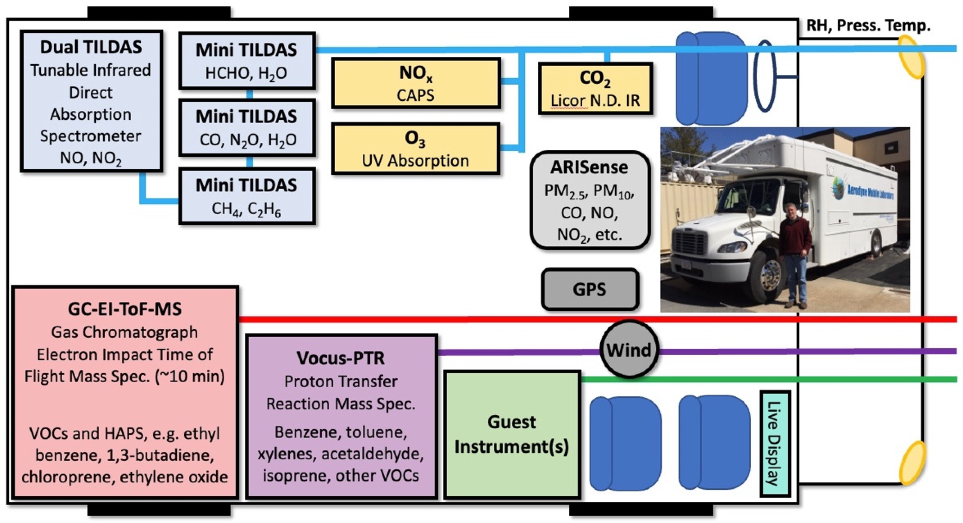
In this study, the Aerodyne Mobile Laboratory (AML) [1,4,6] conducted mobile and stationary measurements of trace gases and VOCs in the SEMI region for six weeks between 21 May 2021 and 30 June 2021, during the MOOSE campaign. The AML was stationed overnight in Dearborn, Michigan, USA at the Salina Elementary School monitoring station operated by the Michigan Department of Environment, Great Lakes and Energy (EGLE). The AML measurements focused on study goals of the CHEmical Source Signatures experiment (CHESS), which included measurement of ozone precursors at key EGLE monitoring stations; and characterization of downwind emission plumes from individual point sources, area sources, and industrial sectors—the topic of this manuscript. Here, we characterize emissions based on the relative molar ratios of species that are enhanced over background in each plume. This is called a “chemical signature” or a “chemical fingerprint”. Next, we examine emissions in a dense industrial area by conducting repeated drive loops under different wind conditions. Finally, we examine plumes from cross-border emissions using measurements from two mobile laboratories. Trends in emission fingerprints and the challenges of emissions characterization in dense industrial areas are discussed.

2. Materials and Methods

2.1. Sampling Plan

The AML sampling plan for the MOOSE project included several goals. In rough order of the percentage of active time, they were: (1) chemical fingerprinting of point sources (CHESS sub-experiment: fingerprinting), (2) co-location with EGLE monitoring stations during expected higher-ozone days (CHESS sub-experiment: ozone precursors), (3) large-scale regional drives sampling the lake breeze front, and (4) coordinated border drives with the Ontario MECP mobile laboratory (TAGA). Day-by-day measurement activities are summarized in Table S1 in the Supplemental Information (SI).
The sampling plan was determined based on daily forecast wind and chemical tracers by Environment and Climate Change Canada (ECCC). Sampling goals aimed to balance point source characterization work with regional measurements involving large-scale transects or stationary sampling collocated with existing state monitoring stations operated by EGLE. These regional measurement days were most often carried out during predicted high-ozone events. A number of coordinated drives were done in conjunction with other MOOSE study participants.

2.2. Instrumentation

The AML hosts a suite of research-grade instruments [1,2,7]. The current version is a diesel truck powered by two additional on-board diesel generators. The AML sampled continuously throughout the 6-week measurement period. When parked overnight at the Dearborn monitoring station, it used on-site power, with AML generators turned off.
Several Tunable Infrared Laser Direct Absorption Spectroscopy (TILDAS) trace-gas monitors from Aerodyne Research, Inc. (Billerica, MA, USA) [8] performed gas-phase measurements of the ambient air, measuring (1) methane (CH4) and ethane (C2H6) [9]; (2) carbon monoxide (CO), nitrous oxide (N2O) and water vapor (H2O); (3) formaldehyde (HCHO) and formic acid (HCOOH) [10]; and (4) nitrogen oxide (NO) and nitrogen dioxide (NO2). A prototype cavity attenuated phase-shift spectrometer for NO2 coupled to an ozone reactor was used to measure total NOx (CAPS-NOx). A 2BTech Model 202 monitor measured ozone (O3) and a Licor Li-6262 gas analyzer was used to detect CO2. Every 15 min, carbon dioxide (CO2) and hydrocarbon-free air (ultra-zero air) was delivered in excess of the intake flow. These gas additions served to spectroscopically background certain TILDAS instruments and check zero values for the other instruments. The TILDAS instruments were operated in series at pressures between 30–50 Torr, with an upstream pressure controller managing flow from a downstream scroll pump (Agilent TriScroll TM 600). TILDAS and other gas-phase calibrations involved precision blending of a known calibration gas (commercially available high-ppm concentration standards with <1% typical uncertainties) with the diluent, ultra-zero air. Additional instrument details are available in the SI, Section S.2.
Fast measurements of volatile organic compounds (VOCs) and oxygenated VOCs (oVOCs) were made using a Vocus Proton-Transfer-Reaction Time-of-flight Mass Spectrometer (Vocus PTR TOF-MS, hereby referred to as Vocus) [11,12]. The Vocus’ focusing ion molecule reactor (fIMR) was operated at a pressure of 2.2 mbar, an axial voltage difference of 600 V, corresponding to an E/N of 125.5. Data was recorded and processed at 1 Hz time resolution using the Tofware software (https://www.tofwerk.com/software/tofware/) (Aerodyne Research Inc. and TOFWERK) in Igor Pro (https://www.wavemetrics.com/products/igorpro) (WaveMetrics, Portland, OR, USA) [13]. Background measurements were conducted every 16 min by overflowing the Vocus inlet with VOC-free air from a zero-air generator (ZAG) with a Pt/Pd catalyst at 400 C. Calibrations were performed every 4 h with a prepared mixture of VOCs (Apel-Riemer Environmental, Miami, FL, USA) diluted with ZAG air. Since the ionization mechanism during this study was the transfer of a proton to the VOCs from the hydronium ion (H3O+), the sensitivities of species in the calibration mixture were correlated to their proton-capture-rate coefficient [14]. Previous studies have shown the efficacy of using this correlation for calibrating signals from the Vocus-PTR instrument [11,15]. To calculate sensitivities for compounds not present in the calibration mixture, the slope of this linear fit was multiplied by the proton-capture-rate coefficient of the species of interest.
The SI (Table S7) lists the high-resolution ion formulas and associated chemical assignments for the Vocus dataset. It is important to note that there may be other species or isomers not listed at a particular mass that may contribute to signal enhancements. Fragments or clusters of the analyte with water or other high-concentration species may also contribute to the signal. As shown by Pagonis et al. [16], even ions that have only one species listed under potential assignments can have contributions from fragmentation of larger parent species. Thus, caution must be exercised when interpreting the identities of all observed Vocus PTR ions. For example, in urban measurements, C6H7+ ions observed in proton transfer spectra are often assigned to benzene. However, as shown in Figure S12 (see Supplementary Materials), direct comparisons of the concentrations obtained for C6H7+ (assuming benzene sensitivities determined from the calibration tank) during MOOSE with those obtained from an onboard gas chromatograph indicate that the C6H7+ ion has multiple contributions in addition to benzene. Ongoing work by Coggon et al. suggest the larger aromatics contribute to this signal [17].
The 2-channel gas chromatograph coupled to an electron-impact ionization high-resolution time-of-flight mass spectrometer (GC-EI-ToF, or simply GC-ToF or GC) [18] reports numerous species, providing expanded coverage for larger hydrocarbons, isomer-resolved VOCs, and halogenated compounds. Measurements are reported every 30 min from a 10-min sample. This data is complementary to the fast measurements reported by the other instruments. Many VOCs that are reported as a sum by Vocus can be isomer resolved by the GC-EI-ToF. The GC-EI-ToF consists of a two-stage thermal-desorption pre-concentration system, followed by a capillary gas chromatography column and a high-resolution time-of-flight mass spectrograph using electron-impact ionization (70 eV). For this campaign, the TOF-MS was operated at nominal mass resolution 3000 Δm/m. The gas chromatograph houses two parallel systems, using identical sample collection (Restek p/n 24090) and sample focusing adsorbent (Markes Int’l p/n U-T15ATA-2S) tubes but different separation columns (Restek Rt-Q-Bond and Rxi-624) for channels 1 and 2, respectively. Channel 1 (Ch 1) is optimized for separation of C3–C4 alkanes, C1–C2 halocarbons and C1–C3 oxygenates. Channel 2 (Ch 2) is optimized for C5–C12 alkanes, C6–C10 aromatics, C3–C6 oxygenates. Both channels can report species beyond those listed above. For final chromatographic data, high-resolution mass spectral fits are generated via TofWare software [13], which produces time series of individual ions. Data is reported as ambient mixing ratio in part-per-billion (ppb), with 0.001 resolution.
GC-ToF instrument sensitivity is a function of sample collection efficiency and detector sensitivity. For field data, the raw response is corrected using sample volume and a measured halocarbon response, using a species presumed to be stable in ambient air throughout the campaign: Ch 1 uses CFC-12 (CF2Cl2) and Ch 2 uses CCl4. For zeros and calibration samples, which will have no ambient halocarbons, a correction factor is based upon linear interpolation from ambient samples that bracket the zero/calibration time period. Additional GC-ToF instrument details are available in the SI.
Inlet lines were mounted to a boom on the front of the AML at a height of 2.8 m above ground for continuous sampling of ambient air. The Vocus inlet was a ~3 m-long 1/4th inch OD PFA Teflon tube with a particle filter on the exterior tip. It had a total flow rate of approximately 5 SLPM, 0.1 SLPM of which was sub-sampled into the instrument. The GC-ToF sampled from a dedicated PFA Teflon inlet, also mounted to the AML boom, with nominal 2 SLPM flow, with 0.16 SLM sub-sampled. All other gas-phase species sampled off the gas-phase inlet, a ½ inch OD PFA Teflon tube with filter inside the AML, and overblow line teed in 6 inches from the inlet tip. A schematic of the instruments and inlet lines is shown in Figure 1.
Wind and select meteorological conditions were measured on the AML boom and rooftop. A Hemisphere (V100) GPS Compass was operated in conjunction with replicate wind sensors (RMYoung 2D ultrasonic anemometer; AIRMAR 200WX WeatherStation).
Real-time data were logged and displayed on monitors in the mobile laboratory, allowing scientists to rapidly detect and follow plumes of interest. Notes were recorded on the same computer and the observer defined and labeled periods of trace-gas data showing enhancements above background (plumes) while in the field. MOOSE data from the AML are available on the National Aeronautics and Space Administration (NASA) Langley Research Center (LARC) website and further archived at the NASA Atmospheric Science Data Center (see Data Availability Statement).

2.3. Calculation of Chemical Fingerprints

In the following sections, we characterize emissions at select facilities based on their chemical signatures. We define a chemical signature as a collection of one or more molar ratios for chemical species or sums of species. Together, these ratios produce a “fingerprint” or “signature” of a given emission. Chemical signatures can be used to compare sites, and to distinguish emissions from neighboring point sources from one another.
Molar ratios are the enhancement in the mixing ratio of a given species A (ΔMRA) divided by the enhancement in mixing ratio of a reference species (ΔMRref) in a given plume:
R a t i o = Δ M R A Δ M R r e f
Ratios are calculated by taking the slope of a scatter plot of the time trace for species A versus the time trace for the reference trace in each plume. The molar ratios in a diluted plume are approximately equal to the ratios in the undiluted emission or stack exhaust so long as those species have much higher concentrations than ambient background concentrations; [19] the plume does not need to be measured at the stack. In the example in Figure 2, we consider the molar ratio of toluene to the sum of C6–C9 aromatics. The time traces (A) show a distinct plume enhanced over background. The correlation plot (B) of toluene versus the sum of C6–C9 aromatics is linear, with a slope of 0.440 and a correlation coefficient of R2 = 0.992. The intercept of the plot is not used in this analysis, but contains information on the background concentrations of the two plotted traces. This method of time trace analysis has been described in detail previously [6,20].
When data from two disparate instruments are considered (e.g., HCHO vs. CH4), it is critical to optimize the time offsets between the traces. This is due to differing delays in the inlet residence times per instrument. Inlet delays are corrected in the published dataset (SI, Section S2) to <1 s accuracy. The inlet delays are then verified plume-by-plume with 0.33 s resolution by cross-correlating each pair of time-traces. When the offset is optimized, the R2 of the linear fit is maximized, and that is the slope taken. For uncorrelated plumes (R2 < 0.65), the original offset is used. This method of time-shifting using correlation plots is commonly used in time series analysis [21].
The choice of denominator for chemical signatures is somewhat arbitrary. Here, the breadth of sources leads us to choose three distinct denominators, for three types of chemical signatures depending on source type: (1) methane, appropriate for natural gas and biogenic sources; (2) carbon monoxide, appropriate for combustion sources; and (3) the sum of C6 to C9 aromatics, appropriate for most solvent, liquid fuel, and some paint sources. Here, C6-aromatic refers to the C6H7+ ion detected by the Vocus PTR-ToF, which is calibrated to benzene, but is also known to contain contributions from fragmentation of higher aromatics (Figure S12 and Coggon et al. [17]). C7-aromatic is the C7H9+ ion, attributed to toluene; C8-aromatics is the C8H11+ ion, attributed to the sum of ethylbenzene and m-, p- and o-xylenes; and C9-aromatics refers to C9H13+, the sum of all aromatic species with the formula C9H12, including propyl benzene, and the various isomers of trimethylbenzene and ethyl methyl benzene. Chemical signatures can be constant through time or can vary with time and site activity. In most cases presented here, the signatures presented are an average of several plumes measured on a given day, or of measurements performed on two or more days. Individual plume signatures tabulated in the supplemental spreadsheet and plume figures shown in the supplemental materials (SI). Facilities have been assigned an arbitrary but unique identifier consisting of the first two letters of their county, followed by a number. Facility coordinates are also available in the supplemental spreadsheet (SI).

3. Results

3.1. Point Source Chemical Fingerprints

Several facility categories were visited during the MOOSE campaign. These include: automakers; steel manufacturers; solvent users; fine chemical manufacturers and chemical waste sites; power plants; biogenic sources such as landfills and waste water treatment plants; natural gas sources such as compressor stations and distribution network natural gas leaks; and oil and gas sources such as refineries and terminal fuel storage tanks.
87 distinct point sources were visited as a part of the MOOSE campaign (Figure 3 and Table S1). Certain large or high-priority sources were visited several times. Not all sources visited exhibited clear or attributable emissions, despite good winds and mobile lab positioning (see discussion), and additional observations would be required to rule out emissions at these sites.
The measurements here consist of concentrations and spatial maps of a vast suite of trace gas, VOC and combustion products. The quantification of emission magnitudes is beyond the scope of this manuscript, though such efforts are underway via inverse modeling efforts by Michigan EGLE [24].
In Table 1, we summarize point source fingerprints for select facilities of different types. The facility ID is listed along with a general category, and a list of noteworthy species. Fingerprint ratios are listed, with the denominator of the molar ratio defined either as the total of C6–C9 aromatics, or as CH4, depending on the source. In the following paragraphs, each listed source is discussed.

3.1.1. MA130: Industrial Coatings

Facility MA130 develops and manufactures coatings for a variety of applications including automotive, pipeline and electrical insulation. An example downwind transect showing chemical ratios is shown in Figure 4. The facility was visited twice, on 23 May 2021 and 4 June 2021 (SI Section S4.1, Figures S13 and S14). There was significant variability in the chemical signatures of this site, even within the same day, particularly in the acetone ratio relative to the sum of aromatics. One possible explanation is that the acetone originates from a different sub-source at the site (e.g., a different room’s stack emissions) than the aromatics. This is consistent with observations of a slightly poorer correlation to the sum (R2 = 0.82, Figure 4) versus any other single aromatic (R2 0.91–0.99, Figure 4).

3.1.2. MA237: Industrial Cleaning

Facility MA237 is an industrial cleaning facility that cleans bulk containers or totes with solvents. It was visited three times, with successful measurements on 15 June 2021 and 25 June 2021 (SI Section S4.2, Figures S15 and S16). Interestingly, at this site, the chemical signature varied significantly between the two visits: C6H7+ enhancements were negligible on 15 June but present on 25 June. Acetone was present on 15 June but absent on 25 June. We observed minor but well-correlated natural gas emissions during these plumes but do not attribute them definitively to the site due to their spatial location.

3.1.3. SA96: Adhesives Manufacturer

Site SA96, an adhesives manufacturer, is dominated by toluene emissions, with minor correlated phenol (C6H7O+ via Vocus-PTR-ToF). SA96 manufactures adhesives, packaging, and construction materials. Some of their products include carton-sealing tapes, house flashing, lumber wrap, mailers, shrink film, and specialty fabrics. Raw materials include polyethylene resin, paper, and adhesives, among others. SA96 was visited on 29 May 2021 and 10 June 2021, with an additional observation on 2 June 2021 en-route to other sites (SI Section S4.3, Figures S17–S22). In 2020, the EPA reported air releases of toluene (982,858 lbs.) from this facility as part of the Toxics Release Inventory Program.

3.1.4. WA236: Chemical Waste

Site WA236 is a chemical waste company with on-site storage. This facility is near several other sources including WA248, a facility treating waste oils and wastewater, and two automaker facilities: WA137, an assembly plant, and WA27, an engine plant Figure S23). The chemical waste site WA236 dominates emissions of aromatics and other VOCs in this area. On several occasions, the AML tracked the plume far into residential neighborhoods (SI Section S4.4, Figures S24 and S25).
The clearest separation of the automaker assembly plant WA137 and chemical waste facility WA236 occurred on 26 May 2021 with wind from the SE (Figure 5). In this figure, a mixed VOC plume (@ symbol) is observed along with a broader, primarily acetone plume (* symbol) further to the north. Sharp and brief spikes of aromatics and CO show the impact of local traffic on these busy boulevards. We attribute the southern-most plume (@ symbol, enhancements of many VOCs) to the WA236 chemical waste facility. The northern-most plume (* symbol, primarily acetone on this day) originates from the automaker assembly plant WA137 or nearby.
Nearly all reported species by the Vocus increase during the plume from this site including C4H9O+ (methyl ethyl ketone + butanal), C3H5O+ (acrolein) and C6H7O+ (phenol). GC-ToF measurements of the WA236 chemical waste site show notable enhancements of halocarbons, primarily dichloromethane (CH2Cl2), aromatics and acetonitrile (CH3CN) (Figure S26). PCBTF, a paint solvent, is also elevated. Positive Matrix Factorization (PMF) [25,26,27,28] was used on the full Vocus mass spectral dataset to separate the chemical waste signature (WA263) from other nearby sources in a plume propagating through the neighborhood (SI Section S4.4, Figures S27–S30). This analysis yielded key ions present in the WA236 plume (Table S8). These ions and their potential chemical assignments are listed in the SI, and include acetone or propanal (m/z 59.049), and select aldehydes or ketones (m/z 73.065).
The sum of the measurements in this area leads us to several conclusions. The chemical waste disposal facility WA236, to the south of the automakers, dominates emissions of aromatics and other VOCs, including odorous oxygenated VOCs, in this area. On several occasions, the mobile lab tracked the plume far into residential neighborhoods. The automaker assembly plant WA137 may also be emitting a mix of acetone and/or aromatic species. Only a few measurements were carried out around WA27, the engine plant, limiting our ability to discern emissions from this site. Several additional sources in this region contribute to a complex source environment, including WA248, the waste oils facility in the same block as the WA236 chemical waste facility, and an unknown VOC source north of WA27 with ppm-level measured aromatic concentrations.

3.1.5. MA141: Natural Gas Compressor Station

Site MA141 is a natural gas compressor station, visited twice on 23 May 2021 and 15 June 2021 (SI Section S4.5, Figure S31). In contrast to many of the other industrial sources described here, MA141 is in a rural area, isolated from other nearby sources, which simplifies measurements and attribution. As expected, the main observed emissions are methane and ethane, the components of natural gas, which are perfectly correlated (R2 = 1.00). The ethane/methane ratio changes slightly between visits, with a ratio of 0.081 on 23 May and a ratio of 0.073 on 15 June, likely reflecting the makeup of the compressed gas itself. These ratios are slightly higher than expected based on Michigan average heating values of natural gas consumed by month of 1058 BTU (May 2021) and 1057 BTU (June 2021) [29]. These heating values correspond to ethane/methane ratios of approximately 0.064 and 0.062, assuming no other components in the gas besides ethane and methane. However, the gas transiting through the MA141 compressor station may not be destined for Michigan consumers or may not reflect the state average. Other species roughly correlated with the natural gas plume are HCHO and NOx; enhancements in CO2 are not clearly distinguishable above instrument noise, and CO is uncorrelated since it is dominated by sharp plumes from other sources such as traffic. For this reason, we report only the ratios of HCHO and NOx to CH4 and only for those plumes with R2 > 0.75. Combustion tracers are expected at compressor stations since the compressor engines themselves run on natural gas, with a certain amount of “slip” (unburned natural gas) escaping with the compressor exhaust [20].

3.1.6. WA238 and WA240: Natural Gas Distribution Network Leaks

Natural gas plumes containing correlated ethane and methane with no other correlated tracers were common in the study area. Two spots in particular (WA238 and WA240) were observed repeatedly throughout the campaign with methane enhancements in the part-per-million level in an area which we refer to as the Dearborn Loop (see Section 3.2 for a more detailed description of this area). Their ethane/methane ratios are summarized in the table below with additional discussion in Section 3.2. The ethane/methane ratios of 0.06–0.09 are similar to those measured at the MA141 compressor station discussed previously and are consistent with the expected ethane/methane ratio in distribution grade natural gas.

3.1.7. WA0 and WA87: Steel Manufacturer and Automaker

Permission was obtained to drive on facility property for a major source area along the Dearborn Loop: the complex comprised of an automaker (Facility WA87) and steel manufacturer (Facility WA0). In the SI (Section S4.6, Figures S32–S38), we describe 5 unique aromatic plume fingerprints, plus a 300 m section of road that showed as many as 4 overlapping plumes with different signatures. This facility duo is complex enough to warrant a dedicated study of its own.

3.1.8. WA22: Refinery

Finally, site access was secured at the refinery in Dearbon (Facility WA22). These results are presented in the SI (SI Section S4.7, Figures S39–S47), and similar to the automaker/steel manufacturer WA87/WA0 described above, demonstrate that no single chemical fingerprint is appropriate for such large and complex facilities. In the following section, we describe an alternate sampling strategy used in the dense industrial area surrounding the refinery and automaker/steel manufacturer.

3.2. VOC Concentrations in an Industrial Area

Dearborn and River Rouge are two cities in Wayne County, Michigan that border Detroit to the west. This area, including the south-western-most part of Detroit, is home to numerous industrial facilities, including automakers, steel manufacturers, a refinery, power generation, terminal stations, rail yards, and more. Residential and shopping areas are in these cities as well. The area is bisected by the Rouge River, a tributary of the Detroit River, used for shipping. The state-run Dearborn monitoring station used as the home base for the mobile laboratory is in this area, and as such, a wealth of measurement data was collected at and around the Dearborn site.
The density of sources in Dearborn and surrounding areas prompted a different sampling strategy than the other point sources targeted during MOOSE. In Dearborn, we defined a standard route that looped through and around the dense source area. This “Dearborn Loop” was repeated multiple times throughout the campaign, at different times of day, and during different dominant wind directions. Such a sampling strategy can allow for triangulation of observed emissions under different wind conditions to a given point source.
Dominant wind directions, as measured at the Dearborn Site were from the SW, SSE, NNW and E directions. The mobile wind measured during these loops shows similar trends, though with less clear distinctions between primary directions, which we attribute to the challenges of measuring wind while driving, and to real wind variability within street canyons. Wind rose plots are shown in the SI, (Section S4, Figures S48 and S49). The wind data suggest defining three general wind flows: Southwesterly (135–270); Northwesterly (270–360); and Easterly (0–135). Figure S50 shows a breakdown of the driven loops by wind direction.
Given the spatial and chemical complexity of sources in this area, we focus on a few key indicators: (1) the sum of C6–C9 aromatics, expected from fuel storage, refinery operations and storage, paint, coatings and solvent use, and combustion; (2) ethane, expected from natural gas leaks, combustion sources, and select refinery sources; and (3) carbon monoxide, expected from traffic, generators, and other industrial combustion sources.
Figure 6 shows Dearborn Loop average concentrations for the sum of aromatics under southwesterly winds. The Dearborn Loop route is about 8.2 square kilometers in size and the bin size is 0.001 decimal degrees. Additional Figures in the SI show analogous maps for other wind directions (SI Section S4.1.1, Figures S51–S53). Under Southerly winds, we see aromatic hotspots downwind (east) of the automaker (Facility WA87) and steel plant (Facility WA0), which are nestled together in the same area. Enhancements are also present downwind of the petroleum terminal (eastern-most section of the refinery outline) and sections of the Rouge River. Aromatic enhancements are also observed on the elevated highway that transects the loop, with the exact location of the enhancements varying depending on wind direction. These highway enhancements could include contributions from highway traffic itself or to Rouge River or refinery sources. Refinery impact is also observed under Northerly flow. Distinct enhancements in aromatics are observed near a petroleum terminal.
Ethane hot spots across all wind directions (SI, Section S4.1.2, Figures S54 and S56) show persistent natural gas leaks at several points of the route. One leak in particular (WA238) was routinely measured under an overpass, where natural gas may have been accumulating. Model estimates of this leak have been performed by Olaguer [30], and this leak and other natural gas distribution leaks were sampled by Batterman et al. [31] Under Southerly flow, a persistent ethane (and CH4) signature was present downwind of a natural gas power generation plant (Facility WA13), but the absence of well-correlated combustion tracers, and the proximity of the transect to the source, suggests a ground-level leak of unburned natural gas.
Finally, CO emissions (SI Section S4.1.3, Figures S57–S59) show persistent enhancements downwind of the automaker and steel complex in both Southwesterly and ENE winds. Enhancements along roadways, particularly the section of elevated highway crossing the River Rouge are evident.

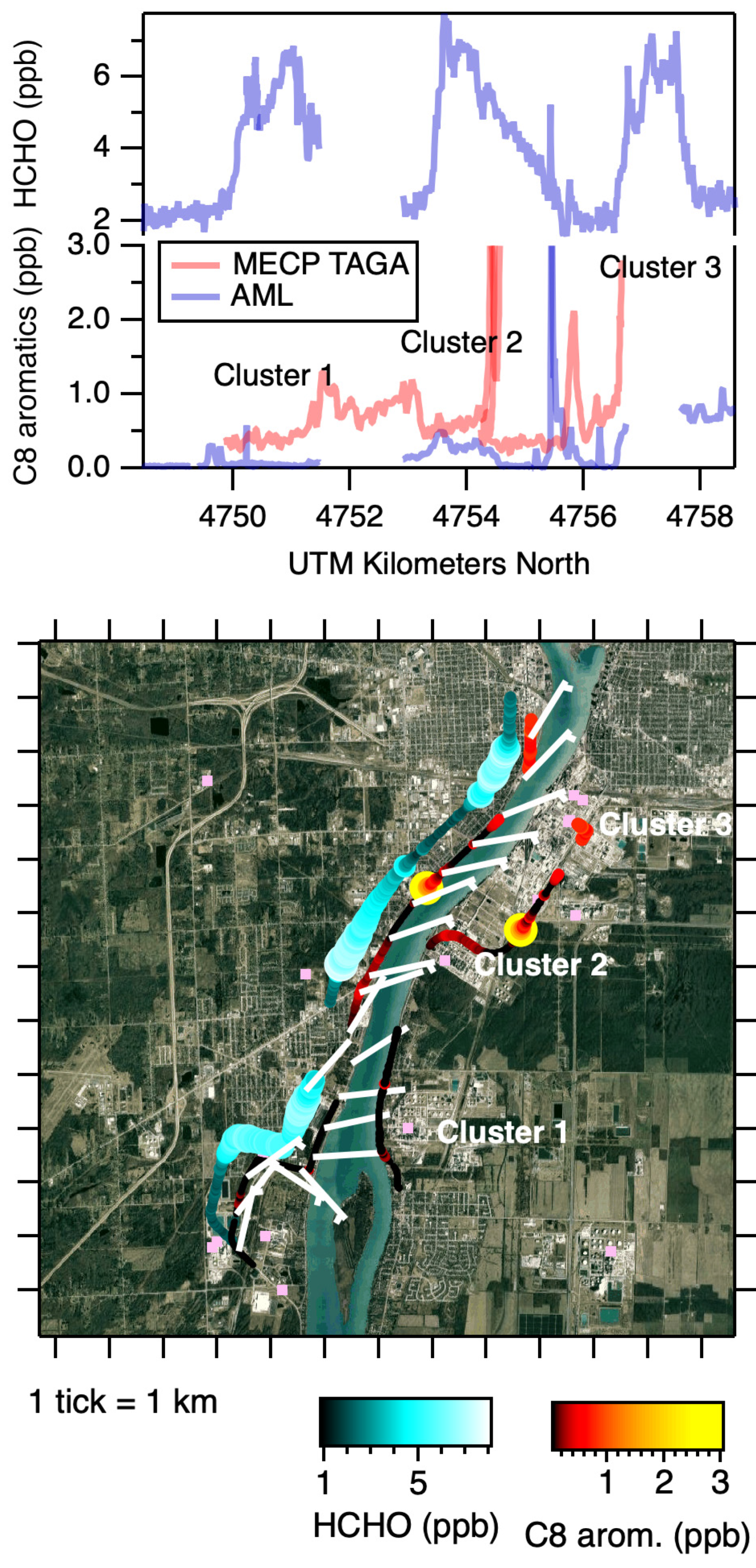
3.3. Cross-Border Emissions

In previous sections, we examined emissions from facilities in the SEMI study area. Here, we show that facilities on the Canadian side of the international border impact the Michigan airshed. The AML spent time sampling in and around Port Huron, Michigan, which is across the St. Clair River from Sarnia, Ontario. Sarnia is home to a dense cluster of refineries and petrochemical facilities [32], and one of the goals of these measurements was to investigate trans-border transport of emissions. Measurements in Port Huron were also coordinated with the Ontario mobile laboratory run by MECP: the Trace Atmospheric Gas Analyzer or TAGA [32]. Both laboratories drove riverside routes at the same time. The Canadian riverside was not accessible for the entire route. No HCHO was available on the TAGA. The SO2 analyzer was not on board the AML during this drive.
Figure 7 below shows a river-side drive of the AML and MECP TAGA from south to north, with dominant winds from the refineries to the East. Though there are numerous individual facilities on the Canadian side, three refineries dominate the area. We number them clusters 1, 2 and 3 from south to north. Just north of Cluster 2 are two additional petrochemical sites: a rubber manufacturer with reported 1,3-butadiene emissions, and a styrene manufacturer. South and inland of Cluster 1 is another petrochemical plant producing ethylene. The map in Figure 7 clearly shows enhancements of aromatics on both sides of the border surrounding Clusters 2 and 3, whereas concentrations are lower near the Cluster 1 facilities to the south.
We also observe three distinct formaldehyde plumes on the US side, with enhancements above background in the 4–5 ppb range. Hydrocarbon and aromatic tracers (C8 aromatics shown) are also enhanced, though not perfectly correlated with the two northern-most plumes associated with clusters 2 and 3. Only modest levels of hydrocarbons and aromatics are observed downwind of the southernmost cluster 1. Figure S61 shows HCHO data as a function of time during this transect along with additional tracers.
The observed enhancements in C8 aromatics downwind of the Cluster 2 area agrees with available emission inventory reports [33]. The Cluster 1 refinery reports 9 tonnes of xylene annually; a refinery in Cluster 2 reports 18 tonnes annually, and for Cluster 3, a refinery/chemical plant reports about 9 tonnes of xylenes annually. However, located in the Cluster 2 area close to the refinery is a separate styrene production facility that releases 14 tonnes of ethylbenzene annually (for comparison the other sites release only 7, 2, and 2 tonnes of ethylbenzene annually). The Cluster 2 area is very much the dominant C8 aromatic release area. Thus, the combined emissions of total C8 aromatics for the three areas are Cluster 1: 16 tonnes, Cluster 2: 34 tonnes, Cluster 3: 11 tonnes.
Next, we investigate the three broad HCHO plumes observed. HCHO emissions may originate from combustion processes, and refinery operations include numerous such processes. Examining the combustion tracers CO and CO2 (Figure S61), and ignoring narrow spikes due to traffic on the drive route, we observe broad increases moderately correlated with HCHO downwind of Cluster 3 and the northern part of Cluster 2, but not with Cluster 1.
A second possible explanation for enhanced HCHO is rapid atmospheric oxidation of reactive alkenes. Formaldehyde plumes have been observed downwind of refineries in Houston, Texas, for example, and attributed to reactive hydrocarbon emissions from refineries [34]. No 1-s data aboard the AML is reported for reactive alkenes, but two 10-min samples measured via GC-EI-ToF showed elevated propene at concentrations ranging from of 0.58–1.9 ppb in Port Huron on this day (background concentrations in Port Huron on this day were about 0.25 ppb, at a time when fast instrumentation showed no VOC plume). The mobile GC measurement of 1.9 ppb included 3-s of exhaust, and so may be contaminated by traffic. However, stationary samples were taken riverside in Port Huron later this day, with wind from the South, yielding propene at 0.58 ppb. These stationary measurements are likely to have sampled Canadian petrochemical Clusters 1 and 2 shown in Figure 7 based on wind direction. A full breakdown of the GC measurements is shown in the SI.

4. Discussion

As part of this study, we observed characteristic emission signatures from different types of industry. Automakers in the study area are characterized largely by VOCs from paint. Automakers also have engine plants, where exhaust measurements are expected, but these emissions were not clearly distinguishable from surrounding traffic, due to the location of such facilities in dense trafficked areas. Industrial/chemical sites (e.g., coatings, solvent use) are characterized by solvent emissions related to their respective processes. Compressor stations are characterized by natural gas emissions and combustion exhaust species. Landfills are dominated by methane and biogenic VOCs without correlated ethane, with some combustion tracers possible depending on combustion equipment on site. Other ubiquitous emission sources not highlighted here include gas stations, and on-road exhaust measurements.
Measured chemical fingerprints can be compared to profiles tabulated in EPA’s SPECIATE database [17]. This database reports emission profiles by weight, to the total weight of VOCs. Industrial solvent emissions, the SPECIATE category that would include the coatings (MA130), industrial cleaning (MA237) and solvent use (SA96) sites lists numerous source signatures or “profiles”. No direct matches are obvious, though the SPECIATE profiles vary dramatically in composition, just as with the range of ratios reported here. Another source category of interest is automotive paint (for example, profile 2546 in SECIATE). Molar ratios to summed aromatics are determined using the reported emissions profile in weight % of total VOCs, and individual species molar masses. The SPECIATE reference signature was dominated by toluene (C7 0.6 molar ratio to C7–C9 aromatics, no benzene reported), then the C8 aromatics (0.3 molar ratio). The C9 molar ratio is 0.1. Acetone had a molar ratio of 0.21 to the summed aromatics. This reference profile is within the measured ratios seen at the WA87/WA0 Automaker/Steel manufacturer for C8 and C9 aromatics, but exceeds the measured ratios for acetone and toluene. We note that other processes besides painting are occurring at this pair of sites, and that the SPECIATE profile predates (1989) the use of low-volatility solvents such as PCBTF.
The measurement of industrial point sources presented several challenges, notably related to source density, source complexity, source height, and the combination of wind direction and road access. Point sources in isolated areas, with surrounding road access and predictable source signatures, were the easiest to characterize. Examples of this type of source include landfills or compressor stations, which tend to be in more rural areas, and have significant emissions dominated by methane. Certain VOC point sources located outside of dense industrial areas also met these criteria, including the industrial cleaning facility MA237, the industrial coatings facility MA130, and the solvent use facility SA96.
The above sources also often were simple in their chemical and spatial emission characteristics (a single central emission point, with just a few chemical species). Other sources measured were much more complex and are better thought of as a collection of point sources. These include the refinery in Dearborn WA22, and the combined automaker/steel plant WA87/WA0. Cross-border refinery and petrochemical emissions from Canada also fall into this more complex category.
For complex sources and dense industrial areas such as Dearborn, neighboring point sources often present overlapping emissions in space. One sampling strategy that was developed was driving repeated loops through these dense areas under different wind conditions. This is discussed in greater detail in Section 3.2. Many of the facilities along this route are large and complex, with no public road access within their fenceline, such as the WA22 refinery and the dual-complex automaker/steel maker (WA87/WA0) at the heart of the loop. Facilities such as these require a dedicated study to completely characterize. Though measurements such dense areas may not fully characterize individual sources, the data collected by the AML during MOOSE is useful in evaluating models by comparing real measured concentrations to gridded model outputs; such modeling efforts may then yield source contributions [24].
Several facilities targeted for analysis had emissions expected from stacks at height. Examples of such facilities include power plants, refineries, and large chemical plants. In the case of power plants, the AML was often able to measure emissions of unburned fuel at ground-level (e.g., ethane and methane leaks at the WA13 power generation plant). Detecting combustion emissions from the stacks, which would require far-away transects in good winds, were most often difficult or impossible to distinguish above traffic and other nearby sources. A section of elevated highway along the Dearborn Loop provided an interesting opportunity to transect a refinery at height; however, refinery emissions proved difficult to distinguish from on-road traffic.
The fingerprints determined here were generally for fresh plumes (minute(s) old), measured near to their respective sources (e.g., hundreds of meters). Most species discussed (e.g., toluene; ethane) have photochemical lifetimes of days or months, and thus do not have time to undergo significant atmospheric processing before being measured. A notable possible exception are the emissions from Canadian refineries (Section 3.3), measured 1–3 km downwind. In that case, we see evidence of propene, a reactive alkene, measured by GC-EI-ToF. We also observe distinct HCHO plumes, a species that can be both directly emitted but also produced as an intermediate in the oxidation of reactive compounds.
Certain facilities targeted for measurement exhibited no clear emissions even under favorable wind and road access conditions. Ruling out emissions from a given facility is much more difficult than a positive detection, particularly in dense source areas. Alternate sampling strategies would be required to rule out emissions from many of these sites, such as direct stack testing, or tracer-release measurements at the site.
Finally, the flexibility afforded by a mobile laboratory allowed scientists to find unexpected sources of emissions such as VOCs and trace them back to their source. In one such example, the WA236 chemical waste facility had emissions that dominated an area that included physically larger and more prominent automakers, and impacted an area spanning several residential and commercial blocks. This example, and others, demonstrate the power of mobile laboratories over stationary sampling in dense industrial areas.

Supplementary Materials

The following supporting information can be downloaded at: https://www.mdpi.com/article/10.3390/atmos14111632/s1, Supplemental figures, including individual plume transects, text and tables: Yacovitch MOOSE Paper SI.docx. Supplemental Spreadsheet, including plume start-stop times, individual chemical fingerprints, site IDs and locations: MOOSERatiosAndSites.xlsx.

Author Contributions

Conceptualization, T.I.Y. and B.M.L.; methodology, T.I.Y., B.M.L. and C.D.; software T.I.Y., J.R.R. and S.C.H.; validation, all authors; formal analysis, T.I.Y., B.M.L., M.R.C., F.M., R.M.H. and J.M.W.; investigation, T.I.Y., B.M.L., C.D., J.R.R., S.C.H., M.R.C., F.M., R.M.H., J.M.W., E.M.L., E.C.F. and M.S.C.; resources, S.C.H.; data curation, T.I.Y., B.M.L., M.R.C., C.D., R.M.H., J.M.W., F.M., E.M.L. and J.R.R.; writing—original draft preparation, T.I.Y.; writing—review and editing, T.I.Y., B.M.L. and R.M.H.; visualization, T.I.Y.; supervision, T.I.Y. and S.C.H.; project administration, T.I.Y.; funding acquisition, T.I.Y. and S.C.H. All authors have read and agreed to the published version of the manuscript.

Funding

Aerodyne Research, Inc. was funded by the U.S. Environmental Protection Agency, grant number XA00E02952, through a subcontract administrated by the Michigan Department of Environment and Great Lakes.

Institutional Review Board Statement

Not applicable.

Data Availability Statement

All mobile laboratory data from the AML and MECP TAGA platforms are publicly available at: https://www-air.larc.nasa.gov/cgi-bin/ArcView/moose.2021?MOBILE=1 (accessed on 23 September 2023) under PI directories: Lerner, Majluf and Yacovitch (AML); and Healy and Wang (MECP TAGA). These data and other associated MOOSE datasets are further archived at https://asdc.larc.nasa.gov/project/MOOSE (accessed on 23 September 2023) under data DOI: 10.5067/ASDC/SUBORBITAL/MOOSE/DATA001.

Acknowledgments

The authors acknowledge Eduardo Olaguer (Michigan Department of Environment, Great Lakes and Energy) and Andrew Snider (Environment and Climate Change Canada) for MOOSE study design and coordination. The authors thank Craig Stroud and colleagues at ECCC for weather and chemical forecasts throughout the campaign; and operators of facilities WA22, WA87 and WA0 for cooperation and assistance during on-site sampling. The authors acknowledge entire MOOSE study team for helpful discussions.

Conflicts of Interest

Aerodyne Research, Inc. is a contract research and instrumentation company. Aerodyne’s participation in the MOOSE study was funded by the U.S. Environmental Protection Agency, grant number XA00E02952, through a subcontract administrated by the Michigan Department of Environment and Great Lakes. The funders had no role in the design of the study; in the collection, analyses, or interpretation of data; in the writing of the manuscript, or in the decision to publish the results.

References

  1. Kolb, C.E.; Herndon, S.C.; McManus, J.B.; Shorter, J.H.; Zahniser, M.S.; Nelson, D.D.; Jayne, J.T.; Canagaratna, M.R.; Worsnop, D.R. Mobile Laboratory with Rapid Response Instruments for Real-time Measurements of Urban and Regional Trace Gas and Particulate Distributions and Emission Source Characteristics. Environ. Sci. Technol. 2004, 38, 5694–5703. [Google Scholar] [CrossRef]
  2. Yacovitch, T.I.; Herndon, S.C.; Roscioli, J.R.; Floerchinger, C.; Knighton, W.B.; Kolb, C.E. Air Pollutant Mapping with a Mobile Laboratory During the BEE-TEX Field Study. Environ. Health Insights 2015, 7–13. [Google Scholar] [CrossRef] [PubMed]
  3. Galarneau, E.; Yacovitch, T.I.; Lerner, B.; Sheppard, A.; Quach, B.-T.; Kuang, W.; Rai, H.; Staebler, R.; Mihele, C.; Vogel, F. From hotspots to background: High-resolution mapping of ethylene oxide in urban air. Atmos. Environ. 2023, 307, 119828. [Google Scholar] [CrossRef]
  4. Yacovitch, T.I.; Daube, C.; Vaughn, T.L.; Bell, C.S.; Roscioli, J.R.; Knighton, W.B.; Nelson, D.D.; Zimmerle, D.; Pétron, G.; Herndon, S.C. Natural gas facility methane emissions: Measurements by tracer flux ratio in two US natural gas producing basins. Elem. Sci. Anth. 2017, 5, 69. [Google Scholar] [CrossRef]
  5. Brantley, H.L.; Thoma, E.D.; Eisele, A.P. Assessment of volatile organic compound and hazardous air pollutant emissions from oil and natural gas well pads using mobile remote and on-site direct measurements. J. Air Waste Manag. Assoc. 2015, 65, 1072–1082. [Google Scholar] [CrossRef] [PubMed]
  6. Roscioli, J.R.; Yacovitch, T.I.; Floerchinger, C.; Mitchell, A.L.; Tkacik, D.S.; Subramanian, R.; Martinez, D.M.; Vaughn, T.L.; Williams, L.; Zimmerle, D.; et al. Measurements of methane emissions from natural gas gathering facilities and processing plants: Measurement methods. Atmos. Meas. Tech. 2015, 8, 2017–2035. [Google Scholar] [CrossRef]
  7. Herndon, S.C.; Jayne, J.T.; Zahniser, M.S.; Worsnop, D.R.; Knighton, B.; Alwine, E.; Lamb, B.K.; Zavala, M.; Nelson, D.D.; McManus, J.B.; et al. Characterization of urban pollutant emission fluxes and ambient concentration distributions using a mobile laboratory with rapid response instrumentation. Faraday Discuss. 2005, 130, 327–339. [Google Scholar] [CrossRef]
  8. McManus, J.B.; Zahniser, M.S.; Nelson, D.D.; Shorter, J.H.; Herndon, S.C.; Jervis, D.; Agnese, M.; McGovern, R.; Yacovitch, T.I.; Roscioli, J.R. Recent progress in laser-based trace gas instruments: Performance and noise analysis. Appl. Phys. B 2015, 119, 203–218. [Google Scholar] [CrossRef]
  9. Yacovitch, T.I.; Herndon, S.C.; Roscioli, J.R.; Floerchinger, C.; McGovern, R.M.; Agnese, M.; Pétron, G.; Kofler, J.; Sweeney, C.; Karion, A.; et al. Demonstration of an Ethane Spectrometer for Methane Source Identification. Environ. Sci. Technol. 2014, 48, 8028–8034. [Google Scholar] [CrossRef]
  10. Spinei, E.; Whitehill, A.; Fried, A.; Tiefengraber, M.; Knepp, T.N.; Herndon, S.; Herman, J.R.; Müller, M.; Abuhassan, N.; Cede, A.; et al. The first evaluation of formaldehyde column observations by improved Pandora spectrometers during the KORUS-AQ field study. Atmos. Meas. Tech. 2018, 11, 4943–4961. [Google Scholar] [CrossRef]
  11. Krechmer, J.; Lopez-Hilfiker, F.; Koss, A.; Hutterli, M.; Stoermer, C.; Deming, B.; Kimmel, J.; Warneke, C.; Holzinger, R.; Jayne, J.; et al. Evaluation of a New Reagent-Ion Source and Focusing Ion–Molecule Reactor for Use in Proton-Transfer-Reaction Mass Spectrometry. Anal. Chem. 2018, 90, 12011–12018. [Google Scholar] [CrossRef]
  12. Riva, M.; Rantala, P.; Krechmer, J.E.; Peräkylä, O.; Zhang, Y.; Heikkinen, L.; Garmash, O.; Yan, C.; Kulmala, M.; Worsnop, D.; et al. Evaluating the performance of five different chemical ionization techniques for detecting gaseous oxygenated organic species. Atmos. Meas. Tech. 2019, 12, 2403–2421. [Google Scholar] [CrossRef]
  13. Stark, H.; Yatavelli, R.L.N.; Thompson, S.L.; Kimmel, J.R.; Cubison, M.J.; Chhabra, P.S.; Canagaratna, M.R.; Jayne, J.T.; Worsnop, D.R.; Jimenez, J.L. Methods to extract molecular and bulk chemical information from series of complex mass spectra with limited mass resolution. Int. J. Mass Spectrom. 2015, 389, 26–38. [Google Scholar] [CrossRef]
  14. Sekimoto, K.; Li, S.-M.; Yuan, B.; Koss, A.; Coggon, M.; Warneke, C.; de Gouw, J. Calculation of the sensitivity of proton-transfer-reaction mass spectrometry (PTR-MS) for organic trace gases using molecular properties. Int. J. Mass Spectrom. 2017, 421, 71–94. [Google Scholar] [CrossRef]
  15. Holzinger, R.; Acton, W.J.F.; Bloss, W.J.; Breitenlechner, M.; Crilley, L.R.; Dusanter, S.; Gonin, M.; Gros, V.; Keutsch, F.N.; Kiendler-Scharr, A.; et al. Validity and limitations of simple reaction kinetics to calculate concentrations of organic compounds from ion counts in PTR-MS. Atmos. Meas. Tech. 2019, 12, 6193–6208. [Google Scholar] [CrossRef]
  16. Pagonis, D.; Sekimoto, K.; de Gouw, J. A Library of Proton-Transfer Reactions of H3O+ Ions Used for Trace Gas Detection. J. Am. Soc. Mass. Spectrom. 2019, 30, 1330–1335. [Google Scholar] [CrossRef] [PubMed]
  17. Coggon, M.M.; Stockwell, C.E.; Claflin, M.S.; Pfannerstill, E.Y.; Lu, X.; Gilman, J.B.; Marcantonio, J.; Cao, C.; Bates, K.; Gkatzelis, G.I.; et al. Identifying and correcting interferences to PTR-ToF-MS measurements of isoprene and other urban volatile organic compounds. EGUsphere 2023, 2023, 1–41. [Google Scholar] [CrossRef]
  18. Claflin, M.S.; Pagonis, D.; Finewax, Z.; Handschy, A.V.; Day, D.A.; Brown, W.L.; Jayne, J.T.; Worsnop, D.R.; Jimenez, J.L.; Ziemann, P.J.; et al. An in situ gas chromatograph with automatic detector switching between PTR- and EI-TOF-MS: Isomer-resolved measurements of indoor air. Atmos. Meas. Tech. 2021, 14, 133–152. [Google Scholar] [CrossRef]
  19. Herndon, S.C.; Nelson, D.D.; Wood, E.C.; Knighton, W.B.; Kolb, C.E.; Kodesh, Z.; Torres, V.M.; Allen, D.T. Application of the Carbon Balance Method to Flare Emissions Characteristics. Ind. Eng. Chem. Res. 2012, 51, 12577–12585. [Google Scholar] [CrossRef]
  20. Subramanian, R.; Williams, L.L.; Vaughn, T.L.; Zimmerle, D.; Roscioli, J.R.; Herndon, S.C.; Yacovitch, T.I.; Floerchinger, C.; Tkacik, D.S.; Mitchell, A.L.; et al. Methane Emissions from Natural Gas Compressor Stations in the Transmission and Storage Sector: Measurements and Comparisons with the EPA Greenhouse Gas Reporting Program Protocol. Environ. Sci. Technol. 2015, 49, 3252–3261. [Google Scholar] [CrossRef]
  21. Wang, J.M.; Jeong, C.H.; Zimmerman, N.; Healy, R.M.; Wang, D.K.; Ke, F.; Evans, G.J. Plume-based analysis of vehicle fleet air pollutant emissions and the contribution from high emitters. Atmos. Meas. Tech. 2015, 8, 3263–3275. [Google Scholar] [CrossRef]
  22. NOAA. Global Self-Consistent, Hierarchical, High-resolution Geography Database (GSHHG); Version 2.2.0; NOAA: Washington, DC, USA, 2013. Available online: https://www.ngdc.noaa.gov/mgg/shorelines/ (accessed on 23 September 2023).
  23. State of Michigan. Michigan Counties; v17a; State of Michigan: Lansing, MI, USA, 2023; Available online: https://gis-michigan.opendata.arcgis.com/datasets/counties-v17a/explore (accessed on 23 September 2023).
  24. Olaguer, E.P. Inverse Modeling of Formaldehyde Emissions and Assessment of Associated Cumulative Ambient Air Exposures at Fine Scale. Atmosphere 2023, 14, 931. [Google Scholar] [CrossRef]
  25. Paatero, P. A weighted non-negative least squares algorithm for three-way ‘PARAFAC’ factor analysis. Chemom. Intell. Lab. Syst. 1997, 38, 223–242. [Google Scholar] [CrossRef]
  26. Paatero, P.; Tapper, U. Positive Matrix Factorization—A Nonnegative Factor Model with Optimal Utilization of Error-Estimates of Data Values. Environmetrics 1994, 5, 111–126. [Google Scholar] [CrossRef]
  27. Lanz, V.A.; Alfarra, M.R.; Baltensperger, U.; Buchmann, B.; Hueglin, C.; Prévôt, A.S.H. Source apportionment of submicron organic aerosols at an urban site by factor analytical modelling of aerosol mass spectra. Atmos. Chem. Phys. 2007, 7, 1503–1522. [Google Scholar] [CrossRef]
  28. Ulbrich, I.M.; Canagaratna, M.R.; Zhang, Q.; Worsnop, D.R.; Jimenez, J.L. Interpretation of organic components from Positive Matrix Factorization of aerosol mass spectrometric data. Atmos. Chem. Phys. 2009, 9, 2891–2918. [Google Scholar] [CrossRef]
  29. U.S. Energy Information Administration. Michigan Heat Content of Natural Gas Deliveries to Consumers (BTU per Cubic Foot). Available online: https://www.eia.gov/dnav/ng/hist/nga_epg0_vgth_smi_btucfm.htm (accessed on 23 September 2023).
  30. Olaguer, E.P. Combining Real-Time Ambient Air Measurements with Inverse Modeling to Estimate Oil and Gas Industry Emissions. EM Mag. Environ. Manag. 2023, 2023, 9–14. [Google Scholar]
  31. Xia, T.; Raneses, J.; Batterman, S. Improving the Performance of Pipeline Leak Detection Algorithms for the Mobile Monitoring of Methane Leaks. Atmosphere 2022, 13, 1043. [Google Scholar] [CrossRef]
  32. Healy, R.M.; Sofowote, U.M.; Wang, J.M.; Chen, Q.; Todd, A. Spatially Resolved Source Apportionment of Industrial VOCs Using a Mobile Monitoring Platform. Atmosphere 2022, 13, 1722. [Google Scholar] [CrossRef]
  33. Government of Canada. National Pollutant Release Inventory (NPRI); Government of Canada: Ottawa, ON, USA, 2021; Available online: https://www.canada.ca/en/services/environment/pollution-waste-management/national-pollutant-release-inventory.html (accessed on 23 September 2023).
  34. Parrish, D.D.; Ryerson, T.B.; Mellqvist, J.; Johansson, J.; Fried, A.; Richter, D.; Walega, J.G.; Washenfelder, R.A.; de Gouw, J.A.; Peischl, J.; et al. Primary and secondary sources of formaldehyde in urban atmospheres: Houston Texas region. Atmos. Chem. Phys. 2012, 12, 3273–3288. [Google Scholar] [CrossRef]
Figure 1. Aerodyne Mobile Laboratory Instrument Manifest for MOOSE-2021.
Atmosphere 14 01632 g001
Figure 2. Time traces (A) and correlation plot (B) of toluene versus the sum of C6–C9 aromatics. The molar ratio is taken from the slope of the correlation plot, m = 0.440.
Atmosphere 14 01632 g002
Figure 3. Overview map of study area showing Michigan and Ontario boundaries. Select cities (blue) and Michigan counties (grey) are labeled. Visited/measured sources are shown as pink dots, with those sources characterized here shown in darker pink and labeled with their site ID. Shorelines: NOAA [22], county lines: State of Michigan [23].
Atmosphere 14 01632 g003
Figure 4. Example chemical fingerprint for Facility MA130. Ratios of VOCs to the sum of aromatics and R2 of the linear fit are listed beside their trace name (top). Additional ratios for other gas phase tracers are noted versus their denominator. Time traces for selected traces are shown (middle). A map (bottom) shows concentration over the driven path.
Atmosphere 14 01632 g004
Figure 5. Representative transects downwind of the chemical waste facility WA236 and the automaker assembly plant WA137. The map (left) shows the AML path colored by acetone concentration. The time traces (right) show a subset of measured species, with traces colored to match the axis labels. For legend of aromatic traces, see Figure 4. A primary VOC plume (@ symbol) is shown, along with a lower intensity and broader plume (* symbol). These plumes correspond to the circled and labeled areas on the map.
Atmosphere 14 01632 g005
Figure 6. Sum of C6–C9 aromatics during Dearborn Loops under SW winds. (A) shows average concentrations. EGLE monitoring stations (purple triangles), inventory sources (white squares) and the outlines of 3 major facilities (WA87—automaker; WA0—steel; WA22—refinery) are also drawn. (B) shows a histogram of the measured concentrations in each map pixel, on a log scale. (C) shows the number of measurements in each map pixel, as well as roads driven over the course of the campaign.
Atmosphere 14 01632 g006
Figure 7. AML and MECP TAGA coordinated transects in Port Huron/Sarnia, from South to North, showing three distinct HCHO plumes, and two broad C8 aromatic plumes. Concentration as a function of kilometers north (top) and maps (bottom) are shown. The drive paths are colored by concentration, with the HCHO trace offset for clarity. The C8-aromatic axes are clipped at 3 ppb to emphasize the broad enhancements over other short-duration events. The petrochemical and refinery sources on the Canadian side of the river are labeled as Clusters 1 through 3. Wind barbs (white) point into the wind. Satellite image source: Google Maps. Imagery ©2023 TerraMetrics.
Atmosphere 14 01632 g007
Table 1. Sample chemical fingerprints for selected source types. Fingerprint ratios are listed for acetone (Ac), aromatics ranging from benzene (C6), toluene (C7), xylenes + ethylbenzene (C8) and the sum of C9-aromatics (C9) which includes trimethylbenzene; ethane (Eth).
Facility IDFacility TypeNoteworthy SpeciesFingerprint
Ratios
Denominator
MA130Industrial CoatingsAcetone, C9-aromaticsAc: 3.17–22.2
C6: 0–0.06
C7: 0.3–0.4
C8: 0–0.06
C9: 0.04–0.6
Total C6–C9 Aromatics
MA237Industrial cleaningC9 and C8-aromatics, acetoneAc: 0–0.14
C6: 0–0.13
C7: 0.30–0.44
C8: 0.05–0.35
C9:0.48–0.23
Total C6–C9 Aromatics
SA96Adhesives ManufacturerToluene, phenol,Ac: 0
C6: 0
C7: 0.99
C8: 0
C9: 0
Phenol: 0.11
Total C6–C9 Aromatics
WA236Chemical WasteAcetone, BTEX, oxygenated VOCs, CH2Cl2
See SI.
Varies. a.
Ac: 1.5–8.4
C6: 0.4–0.18
C7: 0.2–0.8
C8: 0.14–0.6 C9: 0–0.06
Total C6–C9 aromatics
MA141Upstream Oil and GasMethane, ethane, HCHO, NOxEth: 0.073–0.081
HCHO: 8.4 × 10⁻⁴
NOx: 1.6 × 10⁻³
CH4
WA238 and WA 240Distribution Natural GasMethane, ethaneEth: 0.06–0.09CH4
WA87/WA0Automaker/Steel manufacturerC9, C7-aromatics, HCHOVaries. a. See SI
Ac: 0.1
C6: 0.14–0.31
C7: 0.28–0.40
C8: 0.07–0.66
C9: 0.07–0.64
Total C6–C9 aromatics
WA22RefineryBTEXVaries. See SI.Total C6–C9 aromatics
a ranges represent range of ratios in correlated plumes.
Disclaimer/Publisher’s Note: The statements, opinions and data contained in all publications are solely those of the individual author(s) and contributor(s) and not of MDPI and/or the editor(s). MDPI and/or the editor(s) disclaim responsibility for any injury to people or property resulting from any ideas, methods, instructions or products referred to in the content.

