1. Introduction
Extreme weather is defined as small-probability events in which the value of a weather variable is above (or below) a certain upper (lower) threshold within the range of values of the observed variable, and the probability of occurrence is generally less than 10% [
1,
2,
3]. The extreme temperature thresholds in the Qinghai–Tibet plateau region are significantly affected by the terrain. Therefore, to analyze extreme temperatures in this region, the introduction of the concept of relative thresholds is particularly important. Therefore, the 10th and 90th percentiles of climate states are defined as thresholds for extremely low and extremely high temperatures. In recent decades, extreme weather events (torrential rain, heat waves, cold waves, etc.) have been occurring more frequently because of climate change. The economic losses and social impacts caused by such events are huge [
4]. The Qinghai–Tibet plateau is in the transitional region between arid Northwest China, the Qinghai–Tibet alpine region, and the eastern monsoon region. It is affected by the East Asian monsoon, southwest monsoon, and plateau monsoon and is a sensitive and vulnerable area for climate change in China [
5,
6,
7,
8]. Extreme climate events and their changes in the plateau region have unique characteristics [
9] and play an important role in environmental changes in Asia and even the Northern Hemisphere as a whole [
10,
11]. The intensity and frequency of extreme warm events on the plateau have increased in recent years [
12,
13,
14], and the impacts on regional temperature extremes on the plateau have been associated with multiscale temperature variability [
11] and climate change [
15]. Clearly, the influencing factors are complex, and therefore, research about forecasting methods of extreme temperature in the plateau is urgently needed.
Many studies have been carried out regarding extreme weather, such as using “natural time” instead of “conventional clock time” in forecasting extreme weather, which not only made an excellent achievement in air pollution but also in El Nino [
16,
17] and also many studies regarding the extreme temperatures over the Tibetan plateau have been carried out, all of which have shown that predicting Tibetan plateau extreme weather is difficult [
18,
19,
20]. All of them have made a great contribution to forecasting the extreme temperatures over the Tibetan plateau. However, for extreme weather events with low probability and high levels of uncertainty in terms of development, the use of numerical weather models with a single initial value to predict them is far from sufficient. Instead, it is necessary to introduce the concept of ensemble forecasting. As an important direction in the development of numerical forecasting, ensemble forecasting can take into account the uncertainty of initial values and models, and its results reflect various possible changes in future weather conditions, which can provide forecasters with probabilistic information that single deterministic forecasts cannot provide (such as the credibility of the forecast results) [
21,
22,
23,
24,
25,
26]. The probabilistic forecast results provided by this approach can give information on the possibility of extreme events occurring in the future and have better forecasting effects on extreme weather events. Therefore, the method has become an important tool for extreme weather forecasting. However, currently, China’s ability to forecast extreme weather is still relatively weak, and relevant research is urgently needed. With continuous improvements in the numerical prediction of each forecast variable (temperature, precipitation etc.), as well as the ensemble forecast system, forecasters hope to issue early-warning signals for extreme weather. However, it is difficult to achieve this by simply comparing the differences between observations of local meteorological variables and direct forecasts from models [
27]. Accordingly, Lalaurette [
28,
29] used the European Center for Medium-Range Weather Forecasts (ECMWF) ensemble forecasting to develop an extreme weather forecasting method—the Extreme Forecast Index (EFI)—to measure the continuous difference between the ensemble forecast cumulative probability distribution function and the model climate state, as well as sum the difference between the climate state distribution and the forecast distribution. This index has been used by ECMWF and shown to be very useful as an early-warning indicator of extreme events [
30,
31].
To further improve the EFI’s forecasting skill for extreme weather, as well as the ability of its ensemble prediction system to forecast such events, ECMWF uses the same model back-calculation data to update the “model climate” of the EFI and improve its calculation formula to be more sensitive to the information at both ends of the cumulative distribution function, and designed the Shift of Tails (SOT) index as a supplement to the EFI, which is used to indicate the probability of an extreme event relative to the climatological probability [
32], thus enabling the forecasting of extreme weather to be further optimized [
33,
34,
35].
In the present study, the Global/Regional Assimilation and Prediction System (GRAPES) ensemble forecast product, independently developed by China, was used to compare and analyze the effects of adopting different EFI and SOT index thresholds on the forecasting of extreme temperatures in China—especially the plateau region, where extreme temperature changes have indicative significance for China’s climate change. This work aimed to provide forecasters with an ensemble forecasting product that can extract extreme information in their operational work, therefore enabling them to be more confident in the release of early-warning signals of extreme weather.
2. Data and Methods
2.1. Data
This study used historical real-time 2-m temperature ensemble forecast data from January 2019 to December 2020 from GRAPES starting at 12:00 UTC. The schema contained 31 collection members, and the forecast lead times were 24 h, 48 h, 72 h, 96 h, 120 h, 144 h, 168 h, 192 h, 216 h, 240 h, 264 h, 288 h, 312 h, 336 h, and 360 h, spanning a total of 15 days.
Also employed was a 0.5° × 0.5° grid-point dataset of normalized daily temperature from national surface meteorological stations in China as the actual data to compare with the model results. The source of this dataset comprised two parts: (1) China’s National Surface Meteorological Station Normalized Temperature Daily Value Data Set (V1.0) developed by the National Meteorological Information Center and (2) the 2′ × 2′ digital elevation model of China’s land produced by ETOPO5 (Earth topography five-minute grid) Global Surface Relief. In addition, we selected the study area with a terrain height of more than 3000 m (
Figure 1), for which the plateau boundary was based on the ETOPO5 data [
36].
2.2. Methods
To calculate the observed climate percentile, historical data from 1991 to 2020 were used. The calculation date and live field with a sliding time window (7 d) of 3 days before and after the calculation was selected as the climate sequence for sorting in ascending order (the sequence length was 30 yr × 7 d grid points), with each percentile point (0.01, 0.02, …, 0.99, 1) corresponding to a threshold, i.e., the actual climate percentile distribution was a function of grid-point location and time. Due to the short duration of the schema data, there were only data for 2019–2020. However, the schema contained 31 collection members, so the climate percentile calculation of the model forecast field considered the use of multiple ensemble members to increase the number of samples (sequence length was 2 yr × 31 members × 7 d) based on the calculation of the actual field percentile, i.e., the model climate percentile distribution was a function of the grid location, the start time, and the forecast time. Among them, using the data of the model itself to calculate the climate state of the model can make the EFI/SOT index automatically eliminate the systematic deviation of the model, as well as make the extreme events represented by the EFI/SOT index highly correlated with the season. After completing the calculation of the observed and forecasted climatic states, the values corresponding to the 1–100 percentile points of each daily forecast timeliness for each grid point of the nationwide live field and model climate were output. At the beginning of the 21st century, the Intergovernmental Panel on Climate Change (IPCC) provided a clear definition of extreme weather in its third and fourth assessment reports [
37,
38]: extreme weather refers to weather events whose probability of occurrence is less than the 10th percentile of the observed probability density function or exceeds the 90th percentile. In this study, the variable values corresponding to the 10th/90th percentile of the defined climate series were the thresholds for extreme weather.
After continuous updating, the current EFI definition for ECMWF applications is [
25]
where
p is the probability and
is the probability that the ensemble forecast is less than or equal to the “model climate” p-quantile. The weighting
will make
more sensitive to extreme values at both ends. The value of EFI is between −1 and 1, and the closer to −1 the index value, the more extreme and low the forecast event (e.g., extremely low temperature), while the closer the value to 1, the more extreme and high the forecast event (e.g., extreme high temperature or extreme heavy precipitation). When the EFI reaches 1 (−1), it means that all members of the ensemble prediction system forecast are larger (smaller) than the maximum (minimum) value of the model climate state.
Since the EFI integrates the probability of occurrence of different events, resulting in the “loss” of some information, the same EFI does not mean the same probability of an extreme event, so the SOT index is introduced, which is defined as follows:
These formulae represent the relative magnitudes of the quantiles of the ensemble forecast and the maximum and minimum values of the model climatology, representing extreme high and low situations. Among them, and are the maximum and minimum values of the model climate state, respectively, and and are the p-quantiles of the ensemble forecast and the model climate state, respectively. When the 90% quantile of the ensemble forecast () is greater (less than) the 90% quantile of the model climate state (), > −1 (or < −1); and when is greater than the maximum value of the model climate state, i.e., at least 10% of the members of the ensemble forecast are greater than the maximum value of the model climate state, . Essentially, when , it means that for 90% of quantile events of the model climate state, the ensemble forecast probability is greater than the climate probability, and there is a certain possibility of extreme events. The larger the value of , the more member forecasts of the ensemble forecast are greater than the maximum value of the model climate state, i.e., the greater the possibility of extreme events occurring. The case for is similar, indicating the possibility of extremely low-temperature events, so the steps are not repeated.
To be clear, there is a “-” in each forecast lead day in the paper. “-” indicates the meaning of the prediction of the model in advance relative to the test sample, rather than the forecast time, to distinguish between the two time variables.
3. Verification of the Model in Forecasting Extreme Temperatures over the Plateau
3.1. Comparative Analysis of Simulated and Real Climate Extreme Thresholds
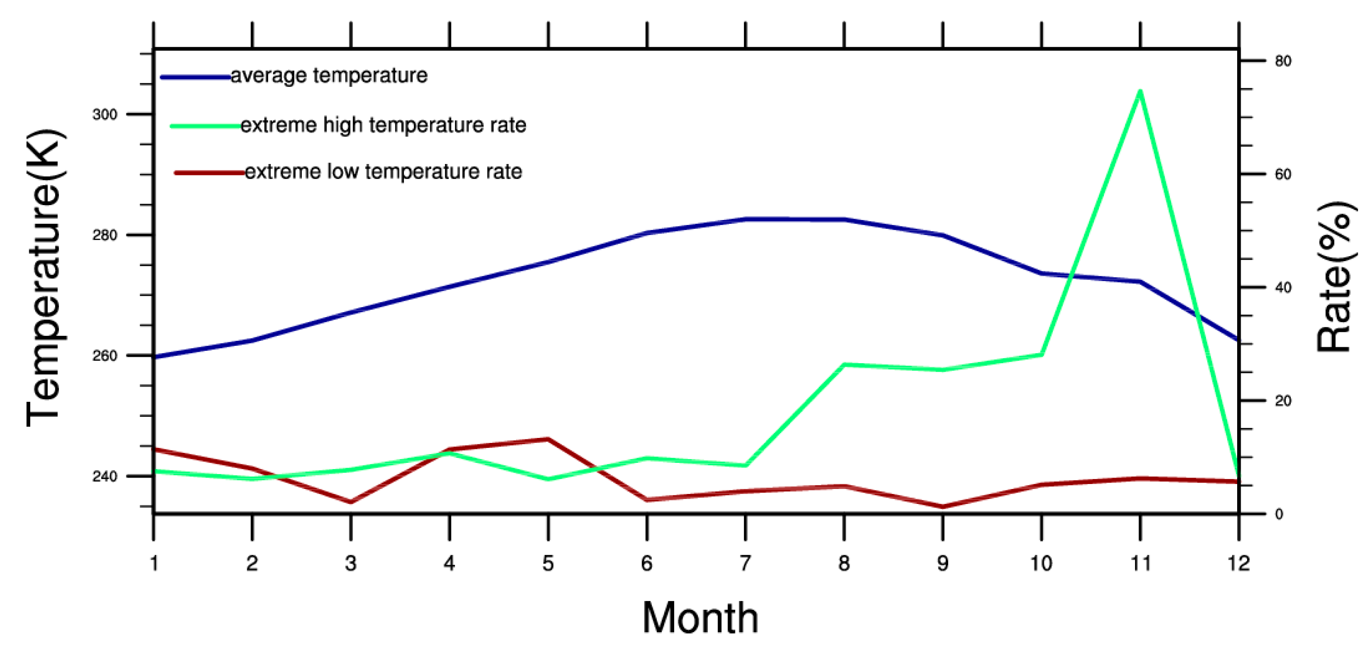
It can be seen from
Figure 2 that the overall temperature in the plateau area is relatively low, the monthly average temperature is between −12 °C and 11 °C, and the monthly variation in temperature presents a unimodal pattern, with high temperatures appearing in July and the lowest temperatures appearing in January. From the distribution of the frequency of extreme temperatures, the frequency of extreme high temperatures in plateau areas is significantly higher than that of extreme low temperatures. This may be due to the impact of global warming. For the plateau region, the occurrence frequency of extremely high temperatures shows an increasing trend after July until November, but it can be seen from the monthly average temperature changes that the temperature in the plateau area shows a monthly declining trend from August onwards. Therefore, June to August is selected as the research period for extremely high temperatures on the plateau. Looking at the monthly changes in the frequency of extremely low temperatures, they occur more often in two periods—namely October–February and April–May. Similarly, since the monthly average temperature in April–May is on the rise, combined with the trend of change in monthly average temperature, December–February is chosen to study extremely low temperatures.
The grid points with an altitude of more than 3000 m were selected as the geographical selection area of the plateau, and the 10th and 90th percentiles of the climate state as the thresholds of extremely low temperature and extremely high temperature to show the thresholds of extreme low temperature in December–February and extreme high temperature in June–September in the plateau area (as seen in
Figure 3). The average extreme low-temperature threshold of the plateau from December to February presents a geographical distribution trend of low in the north and high in the south. The extreme low-temperature threshold of the Kunlun Mountains and Qilian Mountains in the northern part of the plateau is lower than −20 °C; that is, the topography has a more obvious impact on the average temperature in this area, and the extreme low-temperature threshold is lower, but for the high-terrain area in the southwest of the plateau, the extreme low-temperature threshold is higher than that in the north of the plateau. This is related to the data quality for high-altitude temperatures, which also shows that, for areas with high-altitude terrain, such as plateaus, there are greater challenges in terms of the performance of numerical models or the quality of data. Compared with other areas, the analysis of extreme temperatures requires the introduction of the concept of relative thresholds. Judging from the distribution of extreme high-temperature thresholds from June to September for the Tarim Basin and low-altitude areas south of the Hengduan Mountains, the extreme high-temperature thresholds are significantly higher than those in higher-altitude areas. Combined with the analysis of the distribution of extreme low-temperature thresholds, the extreme temperature thresholds in the Qinghai–Tibet plateau region are significantly affected by the terrain, and for the southern plateau region with higher altitudes, the distribution of extreme temperature thresholds is limited by the data quality. Therefore, to analyze extreme temperatures in this region, the introduction of the concept of relative thresholds is particularly important.
3.2. Error Analysis of the Model Climatic State
For the subsequent calculation of the extreme forecast-related indices (i.e., the EFI and SOT index), the matching degree between the model climate state and the historical climate state is crucial, which directly determines the accuracy of the EFI and SOT index. In addition, a comparative analysis of the model climate state and the historical climate state can also test the systematic deviation of the model.
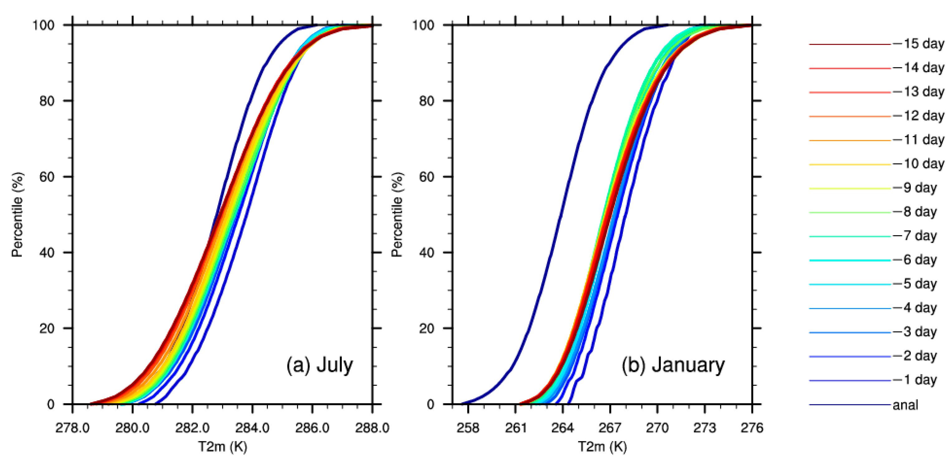
To test the climate percentile of 2-m temperature in summer, we chose July as a representative for analysis. From
Figure 4, we can see from the model deviation for the actual temperature below the 50th percentile that the climatological curves of each lead time are located near the actual climatological curves; that is, the forecast effect of the model on the percentile is better, but the climatological curves under each forecast period are scattered, and the forecast stability of the model is poor. Meanwhile, for temperatures above the 50th percentile, the climate percentile of the model has a certain degree of warm bias, and the climatological curves under each lead time are relatively concentrated; that is, the forecast stability of the model is relatively high. However, for the extremely high temperatures that we are more concerned about in summer, the warm bias of the model is more obvious, and the warm bias decreases slightly with the increase in lead time.
For the equivalent test in winter, the 2-m temperature climate percentile in January is selected. The model has an obvious systematic warm bias; that is, the number of days in advance of the forecast is lower. In addition, the climatic states predicted by the model are all located on the right side of the actual situation; that is, the model climatic states are warmer than the historical climatic states. Regarding the stability of the model, judging from the scatter of the climatological curves for each lead time, the stability of the model is poor, especially for the forecasting of extremely low temperatures, which has a more serious impact. For the 2-m temperature climate state in January, with the increase in lead time, the lower end of the climate state is closer to the actual lower end; that is, as the lead time increases, the overall warm bias of the model’s extreme low-temperature forecast in January decreases, which may be due to the smoother extremes of the model’s forecast as the lead time increases.
3.3. Evaluation of Extreme Temperature Forecast on the Plateau Based on a Simple Ensemble Method
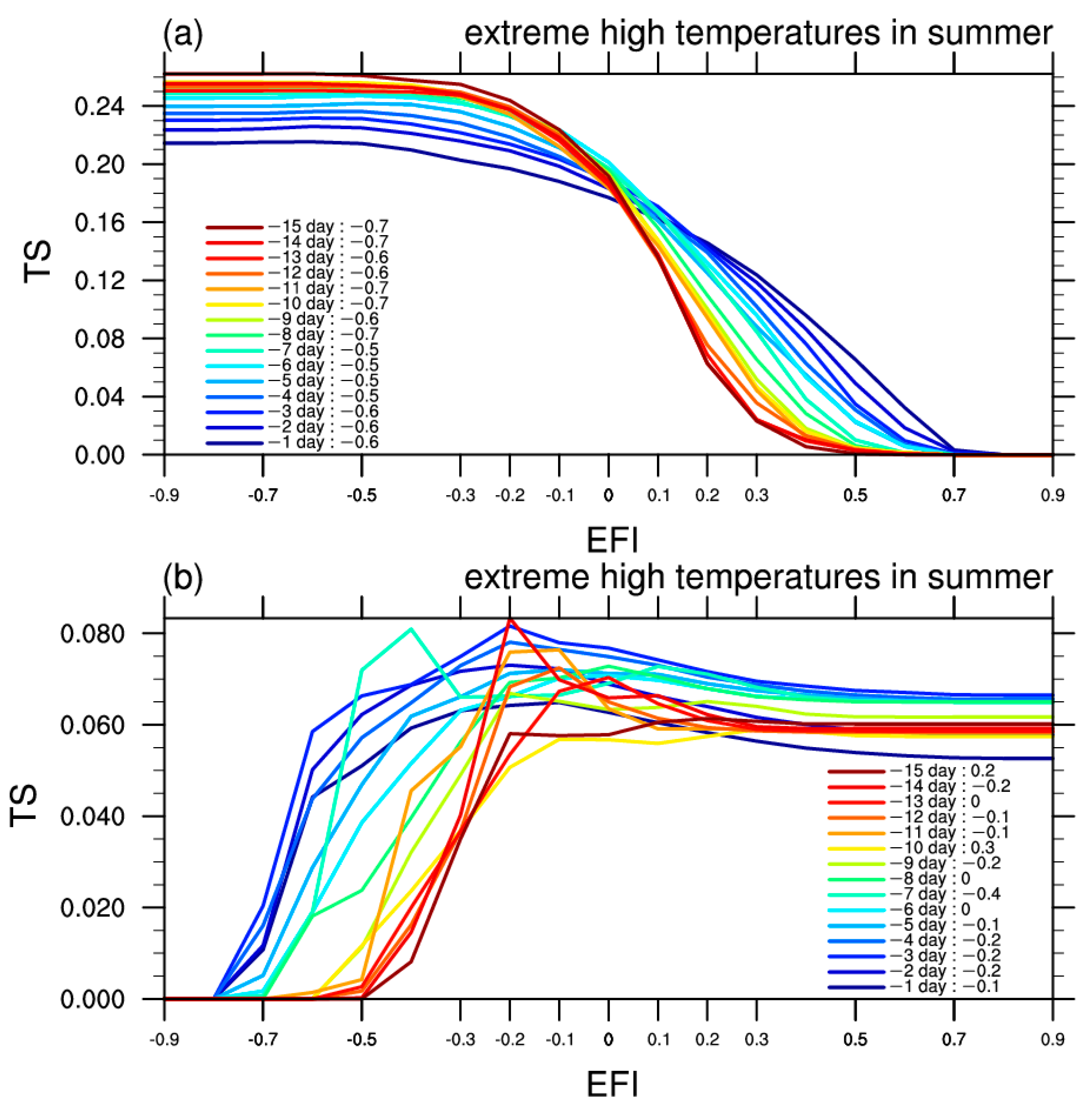
According to the above analysis, it can be seen that, for the average climatological extreme temperature in the plateau region, the threshold values of the model and the actual situation are different, and the difference is different under each lead time. To further illustrate the effect of the model on the extreme temperature forecast in the plateau region, the 90th and 10th percentiles of the climate state are selected as the thresholds of extreme high temperature and extreme low temperature; the arithmetic mean, maximum value, minimum value, and median of the ensemble model are used for deterministic forecasting; and the threat score (TS) is used to test the model forecast.
Using the ensemble mean and ensemble median for forecasting, the TSs for summer extreme high temperature and winter extreme low temperature are relatively close, and the effect of the summer extreme high-temperature forecast shows a consistent downward trend with the forecast lead time. For the forecast of extremely low temperatures in winter, the TS score in the lead time of one to three days increases with the lead time and then shows a consistent downward trend. The TSs from using the maximum and minimum values of the ensemble to forecast extremely high temperatures in summer and extremely low temperatures in winter in the plateau area are higher than those from using the ensemble mean and median. For the extreme high-temperature forecast in summer, the improvement from using the ensemble maximum is particularly obvious, and with the increase in lead time, the TS shows a monotonous increasing trend. For extremely low temperatures in winter, the TS using the ensemble minimum value at lead times of one to five days shows an increasing trend with lead time, while after six days, the TS shows a trend of less movement with lead time (
Figure 5).
It can be seen that, for the forecasting of extremely high temperatures in summer and extremely low temperatures in winter in the plateau region, the effect on the deterministic forecast after processing the ensemble information with the traditional ensemble average is poor. Meanwhile, the TS of forecasting with the ensemble maximum value is higher, but with an increase in lead time, the forecasted TS does not show a monotonous decreasing trend, i.e., for the ensemble forecast model, the extreme information of its forecast is relatively unstable, which also shows the limitations of the model as a whole for extreme temperature forecasting in the plateau region.
5. Conclusions
In this study, based on China’s self-developed GRAPES ensemble forecasting model, the climate states of the model forecast and the real situation were calculated, and the typical months for studying extreme temperatures were selected based on the distribution of the 90th percentile summer and 10th percentile winter thresholds for 2-m temperatures in the real climate state. The model’s ability to forecast extreme events was comprehensively examined by comparing and analyzing the climate state deviations of the model and the real state and by analyzing the computation of extreme temperature TSs using the simple ensemble average, maximum, and median. Second, the EFI and SOT index were calculated, and different forecast thresholds were used to forecast the extreme temperatures under real conditions, which were analyzed with the help of the TS to derive the optimal EFI threshold for the plateau. Meanwhile, to test the predictability of the EFI for extreme temperatures on the plateau, the ROC curve method was used. Finally, a case study was conducted to illustrate the complementarity of the SOT index to the EFI and analyze its applicability in extreme temperature forecasting. The following conclusions were obtained:
(1) For the plateau region, extremely high and extremely low temperatures were analyzed during June–September and December–February, respectively, by combining the month-to-month changes in the monthly average temperature and the frequency of extreme temperature occurrence. Extreme temperature thresholds were significantly affected by the topography, and the introduction of the concept of relative thresholds was found to be particularly important for the southern plateau region, where the distribution of extreme temperature thresholds is limited by the data quality at higher altitudes.
(2) The warm bias of the GRAPES model was more obvious for the forecasting of extremely high temperatures in summer, and the warm bias decreased slightly with the increase in lead time. For extremely low temperatures in winter, there was also a certain warm bias, but the bias decreased with lead time, which may be due to the smoothing of the extremes in the model with the increase in lead time.
(3) For the prediction of extremely high temperatures in summer and extremely low temperatures in winter in the plateau region, the effect of deterministic prediction after processing the ensemble information using the traditional ensemble mean was poor, and the TS of the ensemble maximum was higher. However, with the increase in lead time, the TS of the prediction did not show a monotonous decreasing trend; that is, for the ensemble forecast model, the extreme information of the forecast was more unstable, which also indicates that the extreme information of the model was more unstable with an increase in lead time, i.e., for the ensemble forecasting model, the extreme information of its forecast is unstable, which also indicates the limitation of the model in the forecasting of extreme temperatures in the plateau region as a whole.
(4) The TSs of forecasts with different EFI thresholds were different for different lead times. As the EFI threshold increased, the TS tended to increase and then decrease, which means that there was an optimal EFI threshold. The optimal EFI thresholds for extremely high-temperature forecasts in summer were all less than −0.5, which also verified the warm bias characteristics of the model for extreme high-temperature forecasts. The optimal EFI thresholds for extreme low-temperature forecasts in winter were almost all less than 0.
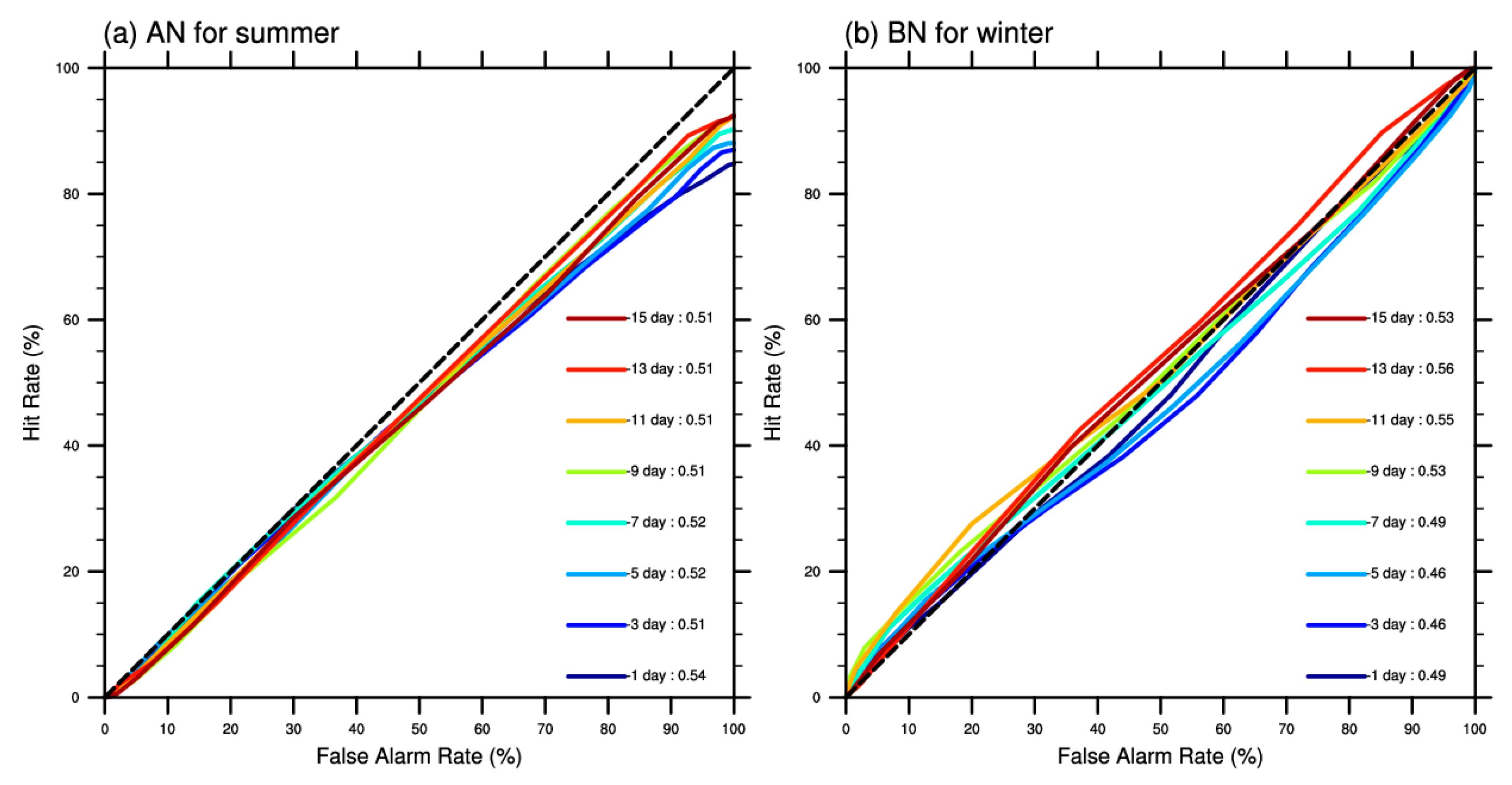
(5) For the GRAPES ensemble model, from the ROC curves, the EFI has a certain level of predictability for extreme summer high temperatures, but the prediction effect is poor. For winter extreme low temperatures, which are poorly predicted by the model itself, post-processing the extreme information predicted by the model using the EFI can improve the forecast effect of the model.
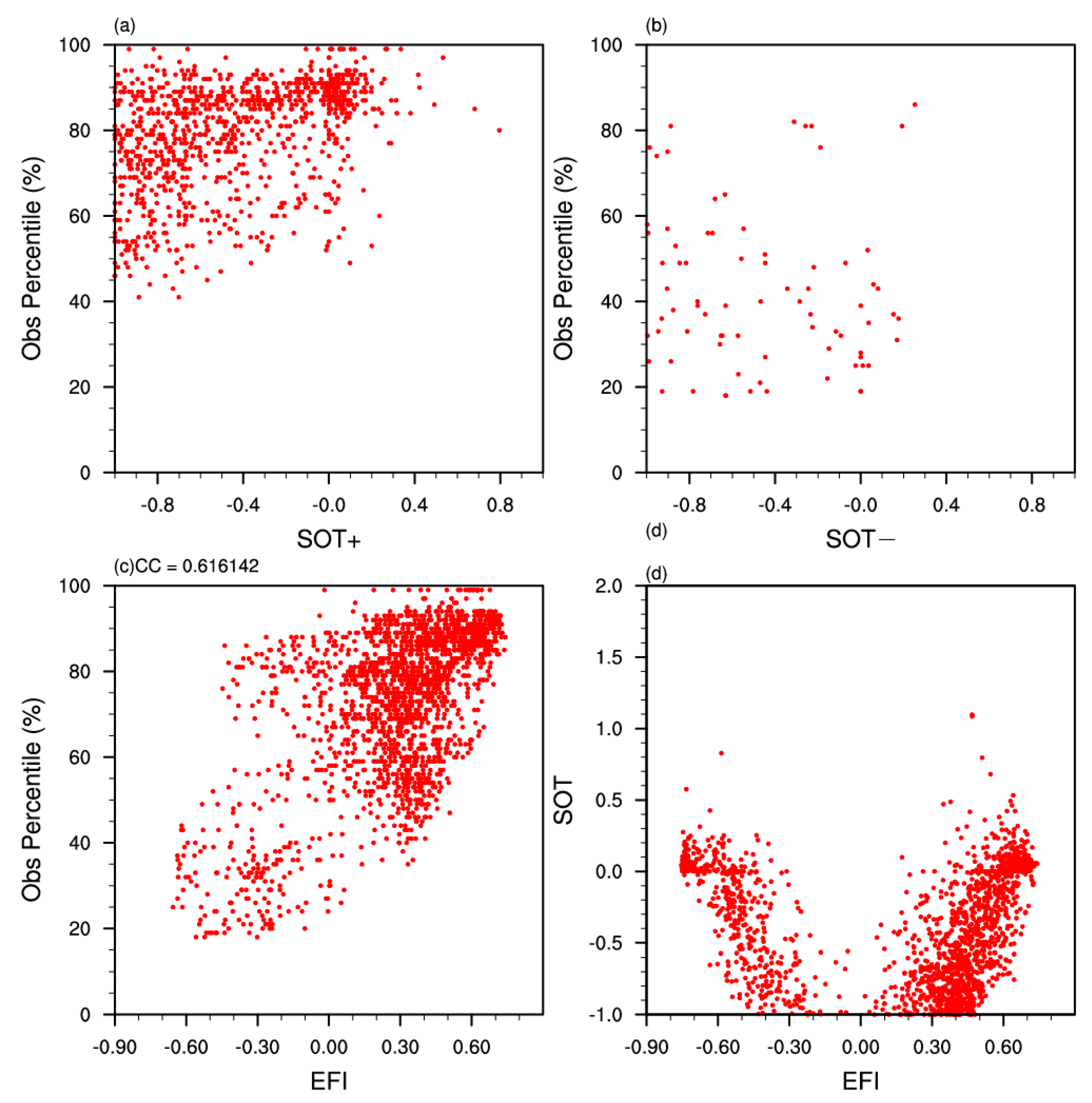
(6) From the analysis of the applicability of the SOT index in individual cases, the extreme intensity reflected by the model through the index to the ensemble members was more obvious for the forecasting of extremely high temperatures in the real situation, but for the forecasting of extremely low temperatures, the extreme intensity indicated by the index of the model was weaker. The extreme information exhibited by the model ensemble members can be somewhat reflected by the EFI for the forecasting of extreme temperatures. Also, when the absolute value of the EFI is large, there is still a large difference in the SOT index, i.e., the SOT index can be a better aid to the prediction of the intensity of extreme events.


