Article

CSES-01 Electron Density Background Characterisation and Preliminary Investigation of Possible Ne Increase before Global Seismicity

1
College of Instrumentation and Electrical Engineering, Jilin University, Changchun 130061, China
2
Istituto Nazionale di Geofisica e Vulcanologia, 00143 Rome, Italy
3
Space Observation Research Center, National Institute of Natural Hazards, Ministry of Emergency Management of China, Beijing 100085, China
4
National Space Science Center, Chinese Academy of Sciences, Beijing 100085, China
*
Author to whom correspondence should be addressed.
Atmosphere 2023, 14(10), 1527; https://doi.org/10.3390/atmos14101527
Submission received: 23 August 2023 / Revised: 26 September 2023 / Accepted: 29 September 2023 / Published: 2 October 2023

Abstract

:
In this paper, we provide a characterisation of the ionosphere from April 2018 to September 2022 for 48 investigated months. We used the data of the China Seismo Electromagnetic Satellite (CSES-01), which is a sun-synchronous satellite with five days of revisit time and fixed local time of about 2 a.m. and 2 p.m. The unique orbit of CSES-01 permitted us to produce a monthly background of the ionosphere for night- and daytime with median values acquired during geomagnetic quiet time in equatorial and mid-latitude regions (i.e., between 50° S and 50° N of geographical latitude). We compared the obtained CSES-01 monthly median values with the solar activity in terms of sunspot numbers, and we found a high correlation of 0.89 for nighttime and 0.85 for daytime between the mean sunspot number and the maximum of the characterised CSES-01 Ne map values. In addition, we extracted all the anomalous positive increases in CSES-01 electron density and compared them with the Worldwide M5.5+ shallow earthquakes. We tested two different definitions of anomaly based on median and interquartile range or (mild) outliers. We tried two relationships between anomalies inside Dobrovolsky’s area before the earthquake and the magnitude of the same seismic events: one which considers distance in space and time and a second which only uses the anticipation time of the anomaly before the earthquake. Using both anomaly definitions, we searched the best coefficients for these two laws for mid-latitude and equational regions. We found that the best coefficients are independent of the anomaly definition, but better accuracy (greater than 80%) is obtained for the outlier definition. Finally, using receiving operating characteristic (ROC) curves, we show that CSES-01 increases seem statistically correlated to the incoming seismic activity.

Graphical Abstract

1. Introduction

In this paper, we deal with the electron density measured in the ionosphere by the China Seismo Electromagnetic Satellite (CSES) to characterise the ionosphere in geomagnetic quiet conditions and propose a preliminary relationship of possible disturbances with seismic activity.

1.1. Ionosphere and Its Characterisation

The ionosphere is the upper part of the atmosphere from about 50 km of altitude up to about 1000 or 2000 km. It is characterised by a partially ionised medium, as suggested by its name. The ionisation is mainly due to solar irradiation by the mechanism of photoionisation [1]. Considering that the driver of this phenomenon is the Sun, the part of the Earth exposed to the Sun (dayside) experiences a higher level of ionisation than the night side. In addition, the normal variability in solar activity (such as the 11-year solar cycle) and abrupt variation due to, for example, solar flares or coronal mass ejection have an impact on the amount of ionisation of the upper atmosphere, i.e., the ionosphere. During the night, the main source of ionisation is the cosmic ray radiation impacting the Earth [2]. Cosmic rays are a secondary source of ionisation during the day, as well as particle precipitation from the magnetosphere, transient luminous effects (e.g., lightning), and meteorites [2].
The presence of this ionised layer that surrounds the Earth is so important that, above all, it permits radio transmission across lengths that are longer than the line of sight (for example, from one continent to another), making de facto possible the first ever trans-oceanic radio transmission by Guglielmo Marconi at the end of the nineteenth century [3].
To monitor the ionosphere, it is possible to use ground antennas and radars. Ionosonde is a ground antenna to monitor the ionosphere, and it produces electromagnetic waves with a sweep of frequency, recording the eventual ionospheric reflected wave. The ionogram obtained by ionosonde reports in the vertical axis the apparent (considering a vacuum medium) altitude of reflection (retrieved by travel time) and in the horizontal axis the tested frequency of the transmitted signal. From the interpretation of the multiple structures observable in the ionogram, it is possible to retrieve the electron density vertical profile in the bottom side of the ionosphere and, in particular, the altitude (hmF2) and electron density (NmF2) of the maximum ionisation peak, named the F2 ionospheric layer, as well as other layers such as the Esporadic E layer [4]. As explained by Huang and Reinisch [5], these techniques have been automated in recent decades to produce estimations of the ionosphere status in real time. This is also possible through the digitalisation of the ionosphere apparatus, sometimes called digisonde, to distinguish it from the analogue version of the antenna [6].
Another way to measure the ionisation of the ionosphere is from in situ Low Earth Orbit (LEO) satellite measurements. These measurements complement the ones obtained from the ground with pro and contra. In fact, the satellite measures the electron density only at one altitude (the one it is flying at) but all over the world. On the other side, the ionosonde has continuous time coverage but only for the observation site. Comparisons and inter-calibrations between the two types of observations are fundamental, for example, those by McNamara et al. [7] for CHAMP satellite data and Peru digisonde observations.
To obtain in situ observations, satellites are generally equipped with Langmuir probes (LP or LAP). An LP is an instrument that, through applying a sweep of current, can measure the classic voltage–current (V-I) curve, and from a non-trivial interpretation of such a curve, the electron density, temperature, and floating electric potential of the plasma can be retrieved [8].
Finally, a similar characterisation of the ionosphere has been presented by Sabbagh et al. [9] and developed with data from the CHAMP and Swarm satellites. The main differences with this paper are that here, thanks to the fixed local time, we do not need a correction of the measurements (that for the cited paper was performed with IRI-2016), and we extended the characterisation to the equatorial region. The investigated years are different as Sabbagh et al. [9] analysed 2004, 2009 (with CHAMP), 2016, and 2017 (with Swarm). Presently, we are investigating the period from April 2018 to September 2022, even though there are some gaps in the data for 2018 due to the commissioning phase of the CSES-01 satellite. Furthermore, in this paper, we limited the analysis to geomagnetic quiet conditions while Sabbagh et al. [9] investigated all geomagnetic activities from G0 to G4 when available. This is because the background we will define is mainly used to retrieve eventual seismo-ionospheric disturbances, and we would avoid any known ionospheric disturbances to avoid confusing possible external source anomalies with internal ones.

1.2. Previous Studies on Seismo-Ionospheric Disturbances

The possible existence of seismo-ionospheric disturbances is a topic widely discussed for several decades, as reported by Chen et al. [10] and Hayakawa et al. [11], including alterations in the lower ionosphere as reported in VLF transmitter–receiver analysis [12], total electron content (TEC) ionospheric pre-earthquake alterations [13], and overall electron density satellite anomalies [14,15]. We would underline that TEC, from the physical point of view, is the vertical integration of the electron density profile. So, the LEO satellites’ electron density measured in situ is strictly linked to TEC. Despite this, the quantities can be sensitive in different ways to ionospheric alterations, so the results can be different.
Several studies involved the DEMETER satellite data, analysing the variations in the equatorial ionospheric anomaly (EIA) possibly induced by an earthquake or other electron density perturbations. These studies were conducted considering a single earthquake or statistical investigations, for example, by Li and Parrot [16] or Ouyang et al. [17], which investigate ULF ionospheric electric field variation related to global seismic activity. Parrot and Pinçon [18] investigated the possible correlation between whistler waves recorded by the DEMETER satellite and shallow (depth ≤ 20 km) earthquakes of magnitude 4.8+ or 5.4+. They identified a statistically significant increase of about 11% in the intensity of whistler activity (originated from lightning) one day before the earthquakes and within 200 km of the epicentre. This supports the lithosphere–atmosphere–ionosphere coupling immediately before the earthquakes. In the same time range is the result of He and Heki [19,20], which proposed that the electron density and TEC can be enhanced 20–40 min before large earthquakes. On the other side, some critics have advanced that the previous result could be an artefact of signal processing due to the co-seismic alterations in the ionosphere by acoustic gravity waves [21].
Previous investigations of possible seismo-ionospheric anomalies in a single case study include among them the Mw = 6.2 L’Aquila (Italy) 2009 earthquake by Piersanti et al. [22], Mw = 6.7 Lushan (China) 2013 by Zhang et al. [23], Mw = 7.8 Nepal 2015 earthquake by De Santis et al. [24], Ghamry et al. [25], Fan et al. [26], Ouzounov et al. [27] and Wu et al. [28], Mw = 6.5 Amatrice-Norcia (Italy) 2016 seismic sequence by Marchetti et al. [29,30], Mw = 7.5 Indonesia 2018 earthquake by Marchetti et al. [31], Mw = 7.6 Papua New Guinea 2019 earthquake by Akhoondzadeh et al. [32], Mw = 7.1 earthquake by De Santis et al. [33] and Marchetti et al. [34,35], Mw = 7.2 Kermadek Islands 2019 earthquake by De Santis et al. [36], and the recent Mw = 7.8 Turkey 2023 earthquake [37]. A recent investigation by Marchetti et al. [38] of the Mw = 3.3 Guidonia (Rome, Italy) small earthquake that occurred on 1 January 2023 does not identify any possible seismo-induced effect, confirming that a lower magnitude event was unlikely to have caused perturbations in the ionosphere, but on the other side it proposed that some Swarm ionospheric disturbances could be related to the Mw = 5.5 event that occurred in November 2022 in the Adriatic sea. Generally, the cited studies identified an increase in electron density absolute value or some variations in its value. Some studies are also corroborated with magnetic field satellite data (from Swarm or CSES). Still, the anomalies are generally identified at different times underlying different possible lithosphere, atmosphere, and ionosphere coupling mechanisms, as Zhang et al. [39] concluded for the Lushan (China) 2013 earthquake.
Important research, the results of which will be extended in this paper on satellite data, is investigating the possible relationship between the space–time distance of ionospheric anomalies and earthquake magnitude. Korsunova and Khegai [39], analysing ionosonde data and earthquakes in Japan, found that the logarithm of the product of the distance in km and the time in advance in days is directly proportional to the earthquake magnitude. Perrone et al. [40,41] confirmed this result for Italy and Greece, and more recent studies applied and established this relationship for seismic events in Italy in 2016 [42].
On the other hand, several statistical studies have been performed with Swarm and CSES satellite data. For Swarm, we would like to note here the results of De Santis et al. [43], expanded in Marchetti et al. [44], which not only identified a statistically significant increase in magnetic and electron density anomalies before the M5.5+ shallow (depth ≤ 50 km) worldwide earthquake but also identified a similar relationship to the one observed by Korsunova, Khegai, and Perrone, in this case finding that the logarithm of the anticipation time of magnetic anomalies increases with the magnitude of the incoming earthquake. This law was previously found by Rikitake et al. for several ground earthquake precursors [45]. Statistical studies dedicated to electron density from DEMETER have been performed by Yan et al. [46], identifying a statistically significant increase in anomalies about 5–6 days before M5+ earthquakes. De Santis et al. [47] and Marchetti et al. [34] correlated electron density variations measured by CSES LAP with M5.5+ shallow (depth ≤ 50 km) earthquakes. They identified an increase in anomalies 20 days before the earthquakes and that the anomalies in the three months before earthquakes are more numerous than the ones recorded in the three months after the earthquakes, suggesting that the difference may underline the LAIC effects of the preparation of the investigated earthquakes. The main difference with this paper is that here, we will investigate the absolute value of electron density, while previous studies explored the variations around the mean value. Ouzounov [48] defined this type of anomaly as “absolute” and the other one as a “relative” anomaly. A recent paper in this direction has been published recently by Han et al. investigating the variations in electron density of the CSES, identifying an interesting distribution of the directions of the anomalies with respect to their epicentres, i.e., toward the geomagnetic equator [49].
With regard to the physical mechanism which could induce ionospheric disturbances as an increase in electron density, several theories have been proposed. One of the most promising ones is based on the release of p-holes (positive holes by Freund [50,51]) for the increase in the stress that can break the peroxy chemical links on the rocks. The release of p-holes can induce electromagnetic radiation in the ultra-low-frequency (ULF) range or create a statical electric field at the Earth’s surface, which could alter the ionospheric electron density as physically and numerically simulated by Kuo et al. [52]. Other hypotheses are based on the release of geo-gases (e.g., Etiope and Martinelli [53]) or radon, which could ionise the atmosphere and alter the global electric circuit, such as that proposed by Pulinets and Ouzounov [54].
Such geophysical studies must be integrated with engineering assessments and improvements of buildings and infrastructures, especially critical ones such as bridges [55]. In fact, such infrastructures are critical to a quick response to an eventual disaster.

1.3. CSES Satellite Mission

The China Seismo Electromagnetic Satellite (CSES-01, also known as Zhangheng-01) is a mission of the China National Space Administration (CNSA) developed in cooperation with the Italian Space Agency (ASI). The mission plan is to launch a constellation of satellites dedicated to monitoring from the ionosphere the possible signals induced by seismic activities on the Earth [56]. On 2 February 2018, China successfully launched the first constellation satellite, CSES-01. It is equipped with multiple payloads to monitor the geomagnetic and electric fields, ionosphere plasma properties and composition, and detect particle bursts by two complementary (for energy range and orientation) particle detectors, the high-energy particle package (HEPP) and the high-energy particle detector (HEPD). The last one was provided by ASI and built in a consortium coordinated by the Italian National Institute of Nuclear Physics (INFN) [57]. CSES-01 is the first ever satellite launched by China for this purpose, and it combines the previous experience of the DEMETER satellite launched by France for this purpose in 2004, flying up to 2010, and also from the Swarm mission [58,59]. CSES-01, analogously to the DEMETER, is inserted in a Sun-synchronous orbit, which is an important point in order to construct a reliable satellite background without the necessity of applying corrections for the measured local time. CSES-01 has two operational modes: burst and survey; the first is applied in seismic active regions (seismic belt) and China, while the second is in the rest of the world. In particular, CSES-01 is equipped with a LAP instrument composed of two probes with different dimensions (sensor spheres of 5 cm and 1 cm) in order to match the different levels of electron density present in the ionosphere (the first is a high-gain probe and the second is a lower gain one) [60]. The frequency resolution of the CSES-01 LAP data is 1.5 s/sample in burst mode and 3.0 s/sample in survey operational mode. In this paper, we investigated the LAP data acquired by CSES-01. There is an open debate on the absolute calibration of these satellite data due to a discrepancy with Swarm LP measurements, without reaching a clear conclusion [61,62]. Anyway, the most important is that, as affirmed by Yan et al. [61] and confirmed by other studies, for example, Marchetti et al. [31], the actual electron density profiles of CSES-01 are well in agreement with the Swarm satellite and empirical Ionospheric Reference International (IRI) model [63]. Considering that here we are not comparing the absolute value of electron density with other satellites or measurements and that CSES-01 LAP data are auto-consistent, we consider the discussion on the absolute value to be beyond the scope of the present paper as not influencing the conclusions of the presented analyses. The observations of CSES-01 not only provide important results for a better understanding of earthquakes, but they permit to investigate and comprehend other geophysical phenomena such as geomagnetic storms [64,65], volcano eruptions (for example, the La Palma 2021 eruption [66] and the extreme explosion on 15 January 2022 of the Hunga Tonga-Hunga Ha’Apai volcano [34,67]), or magnetic pulsations Pi2 [68]. The magnetic data of the CSES also contributed to the 13° generation of the IGRF geomagnetic model [69] and provided an independent model for equatorial regions [70]. In addition, CSES-01 data from several payloads permitted a deep study of equatorial plasma bubbles by Gou et al. [71].

2. Materials and Methods

This paper analysed the LAP (Langmuir probe) data from the CSES-01 satellite. They are provided in a level 2 data product at a frequency of 1 sample/1.5 s in burst mode or 1 sample/3.0 s in survey mode. We analysed the available data without resampling for the different frequencies. Figure 1 shows an example of 5 days of electron density divided into nighttime and daytime. We show in this example 5 days to cover the different orbits of the CSES-01 after they are repeated, and we selected a geomagnetic quiet time for reference. The overall workflow of the extraction of anomalies and their correlation with earthquakes is provided in Figure 2. It is composed of several steps described in specific subsections and summarised in the following list:
  • Data organisation by cells, regions, and local time;
  • Data selection in geomagnetic quiet time;
  • Background estimation end extraction of samples with higher Ne;
  • Preparation of the earthquake catalogue;
  • Declustering of the high Ne samples;
  • Extraction of the anomalies;
  • Testing the possible relationship between the distance and anticipation time of anomalies and earthquake magnitude;
  • Assessment of prediction capability with confusion matrix and ROC curves.
A list of the parameters used is provided in Appendix B.

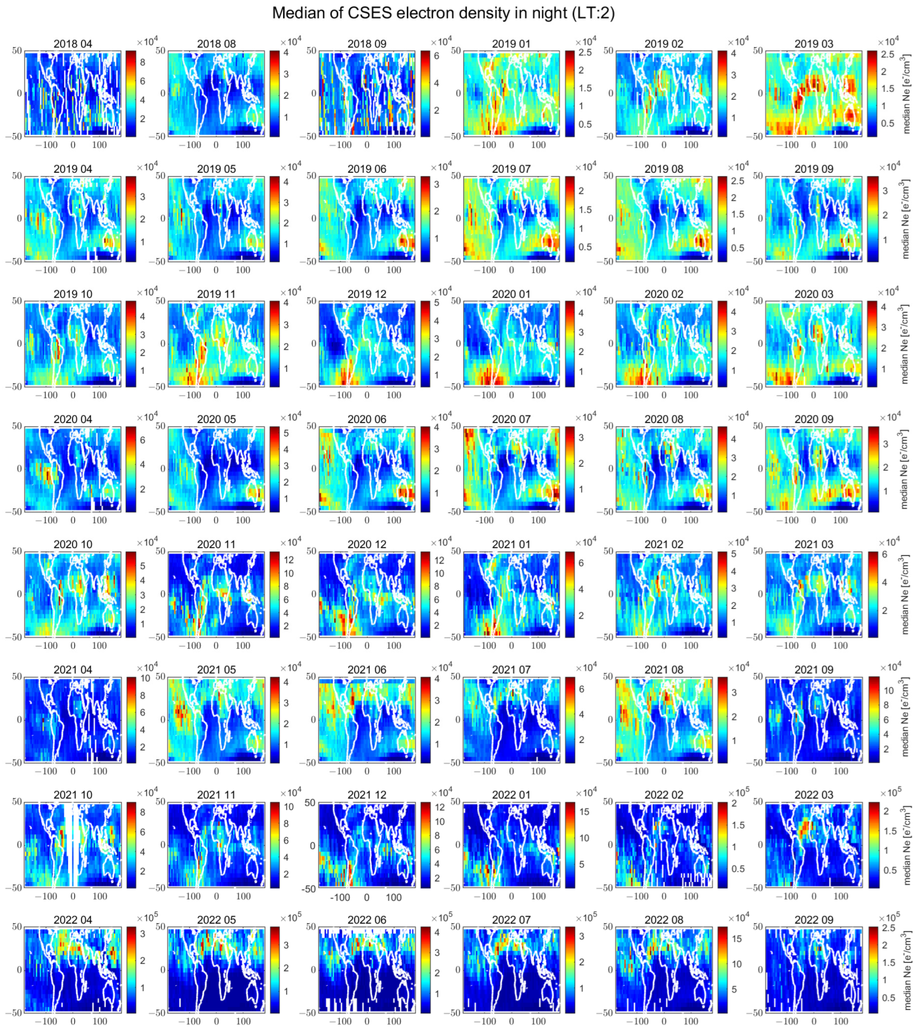
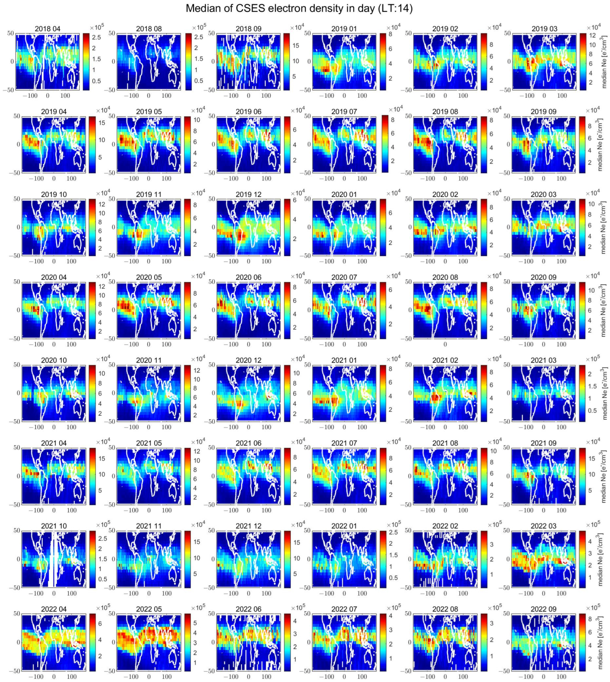
2.1. Background Characterisation

2.1.1. Data Organisation by Cells, Regions, and Local Time

We consider the data acquired at mid-latitude and equatorial regions. In particular, mid-latitude is from 35° N to 50° N for the Northern Hemisphere and from 50° S to 35° S for the Southern Hemisphere, and the equatorial region is from 35° S to 35° N geographic latitude. In order to construct a background, we divided the investigated region into square boxes of 5° latitude × 5° longitude (see Figure 1 for the representation of the boxes). We should underline that this background is limited to the altitude of the CSES-01 satellite, which is about 515 km.
For the background characterisation, the data are divided into months and local time (night or day). We found that cell size of 5° latitude × 5° longitude may be a good compromise to use one month of time resolution background and retain a sufficient number of samples to calculate the statistics. Considering that the CSES-01 is Sun-synchronous, the observed local time is fixed for the night as 2 a.m. (at the equator) and for the day as 2 p.m. (at the equator). Other parts of the track are some minutes in advance of or behind local time (~±15 min of shift with respect to the reference), but the shift is constant for all the missions, so the data in the same boxes are perfectly comparable.

2.1.2. Data Selection in Geomagnetic Quiet Time

In this work, we considered only geomagnetic quiet time conditions because the final goal of the background is to extract possible pre-earthquake anomalies. As the possible pre-earthquake anomalies are expected to be weaker signals, we consider it better to exclude the time perturbed by geomagnetic activity in order not to confuse internal anomalies with external ones. Some studies, for example, Fan et al. [26], tried to investigate the full time by separating the possible sources of the signal by sophisticated algorithms, but this goal is beyond the scope of this paper, and the method is not applicable to searching the absolute anomalies, the object of this research. The geomagnetic quiet conditions are defined as a function of the region, as we considered that polar geomagnetic activity can penetrate at mid-latitude with electric penetrating currents. We monitored it using the Auroral Electrojet (AE) index. In addition, the Dst (disturbance storm) index is measured with four geomagnetic ground observatories placed around the geomagnetic equator, and it is a global indication of the geomagnetic storm activity affecting our planet [72]. Finally, the whole planet’s geomagnetic activity is also represented by the ap geomagnetic index, a linear planetary index calculated from the logarithmic scale index Kp [73]. In addition, we consider not only the data acquisition time but also the previous hours as they can have a consequence on the time of acquisition due to a delay in the ionosphere’s recovery from perturbed conditions. In detail, we selected geomagnetic quiet time data in:
  • The equatorial region with ap ≤ 32 nT in the previous 24 h, |Dst| ≤ 20 nT during acquisition, and |Dst| ≤ 30 nT in the previous 24 h.
  • The mid-latitude region with ap ≤ 32 nT, |Dst| ≤ 20 nT during acquisition, |Dst| ≤ 30 nT in the previous 24 h, AE ≤ 300 nT in the previous 6 h, and AE ≤ 200 nT during the acquisition.
The threshold on the ap geomagnetic index corresponds to the G0 quiet level defined by NOAA (https://www.swpc.noaa.gov/noaa-scales-explanation, last accessed on 23 August 2023).

2.1.3. Background Estimation End Extraction of Samples with Higher Ne

The background for day or nighttime local time and the specific box is constructed if at least 10 samples are in the box and the median “M”, interquartile range “IQR”, and “Q3” (75th percentile) are estimated. The single satellite values that positively exceed the M + kt1 × IQR (with kt1 = 0.5) threshold are stored and extracted for the subsequent comparison with the earthquakes. We should underline that these samples are not the “anomalies”, but a pre-selection of higher Ne values that will be the source of further processing in the search for anomalies.

2.2. Correlation of Electron Density Anomalies with Earthquakes

In this section, we will correlate the extracted samples from the previous section with the earthquakes.

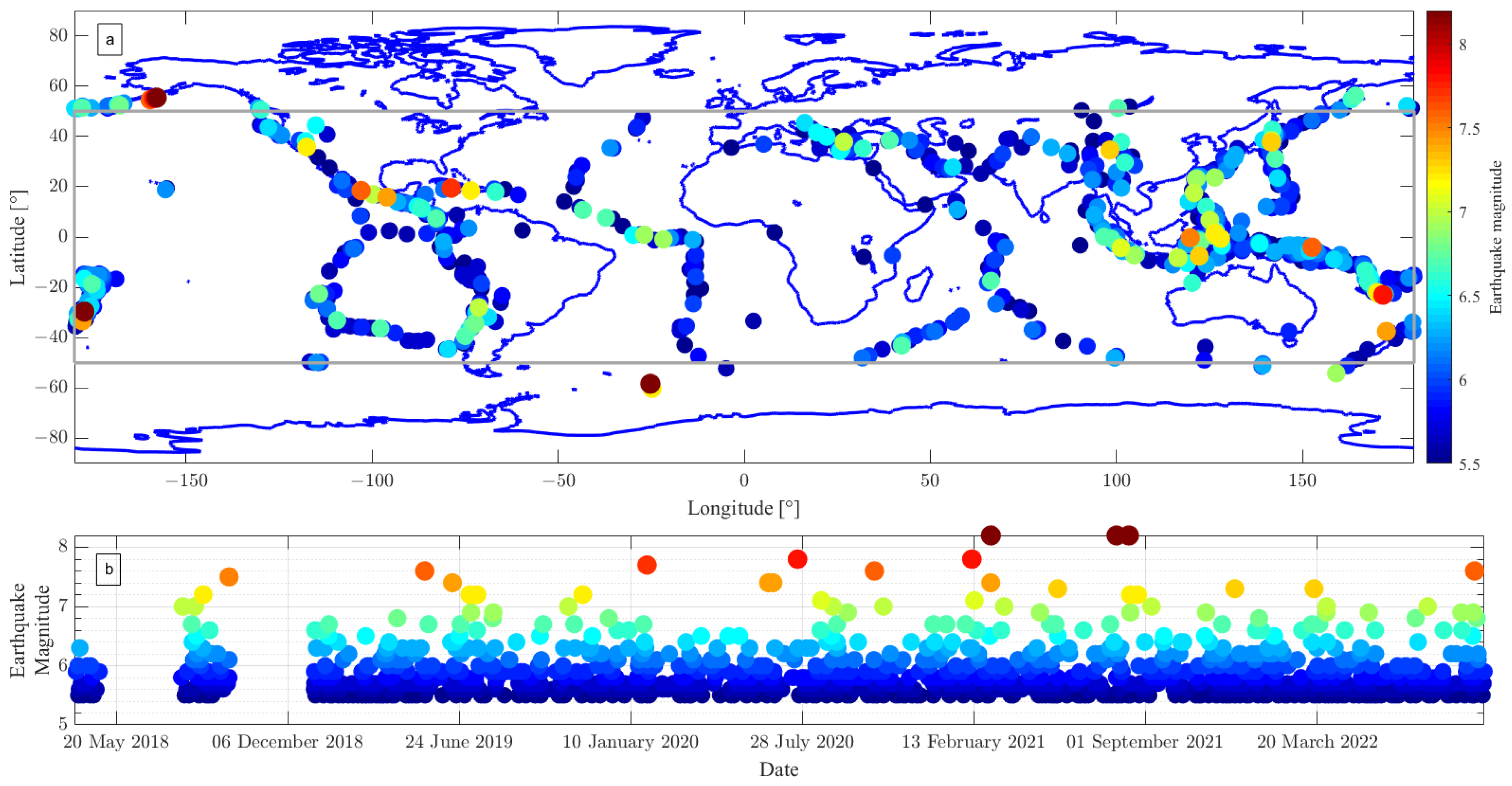
2.2.1. Preparation of the Earthquake Catalogue

We selected the earthquakes from the USGS catalogue, extracting the event at any depth with a magnitude equal to or greater than 5.0. The catalogue has been then declustered by Reasenberg’s [74] method using a window of 20 days before and 10 days after. Then, it was cut at a 50 km maximum depth and minimum magnitude of 5.5. The catalogue was processed by Z-Map software, version 7 [75]. Finally, we consider only the M5.5+ shallow earthquakes. Figure 3 represents their geographical and temporal distribution. The prepared catalogue is analogous to the one used by De Santis et al. [43,47] and exactly the same (just extended for time) as that in Marchetti et al. [34,44].

2.2.2. Declustering of the High Ne Samples

The anomalous samples extracted from the previous processing can be one or more anomalies. In fact, an anomaly that has an extension in latitude (for example, of some degrees) will be depicted as several contiguous anomalous samples. To avoid overcounting the anomalies, the extracted anomalous samples have been declustered by an opposite algorithm that compares the distance of the anomalous samples extracted on the same day, and if two samples are less than 1.0° apart, they will be considered the same anomaly (or the same cluster). The concept is extended to a cluster of anomalies composed of 2 anomalous samples or any higher number of samples. Finally, we prepared a declustered anomaly catalogue containing all the independent anomalous samples (not part of any cluster). For the cluster, only one item that corresponds to the average of all quantities (position, time, and overall detection threshold) is included.

2.2.3. Extraction of the Anomalies

After declustering the Ne anomalies, we applied the final threshold kt2 to extract the effective anomalous values we will compare with the earthquakes. In this work, we tested two approaches commonly used to define anomalies:
  • Anomaly = Ne > Median + kt2 × IQR;
  • Anomaly = Ne > Q3 + kt2 × IQR (if kt2 = 1.5, this is the definition of a mild positive outlier).
We should underline that “kt2” is the final threshold used to define anomalies, while “kt1” is a technical threshold to pre-select only some satellite samples (potentially anomalous) in order to reduce the amount of data and increase the computational efficiency.

2.2.4. Testing the Possible Relationship between the Distance and Anticipation Time of Anomalies and Earthquake Magnitude

The final Ne anomalies are then compared with the earthquakes. In particular, for each earthquake of magnitude M, all the anomalies that occurred in Dobrovolsky’s area defined with Dobrovolsky’s radius in kilometres rDob = 10(0.43 × M) before the earthquake are extracted. For each anomaly, the following two quantities are calculated: the first one is related to the relationship introduced by Korsunova–Khegai–Perrone [39,40,41,42] for ionosonde multiparametric anomalies, while the second one is extrapolated from Rikitake’s law [45] for earthquake precursors:
  • Log10(ΔT × R); decimal logarithm of the product of anticipation time “ΔT” in days of the anomaly with respect to the earthquake and distance “R” in kilometres of the anomaly and the earthquake.
  • Log10(ΔT);
  • The above quantities are compared with:
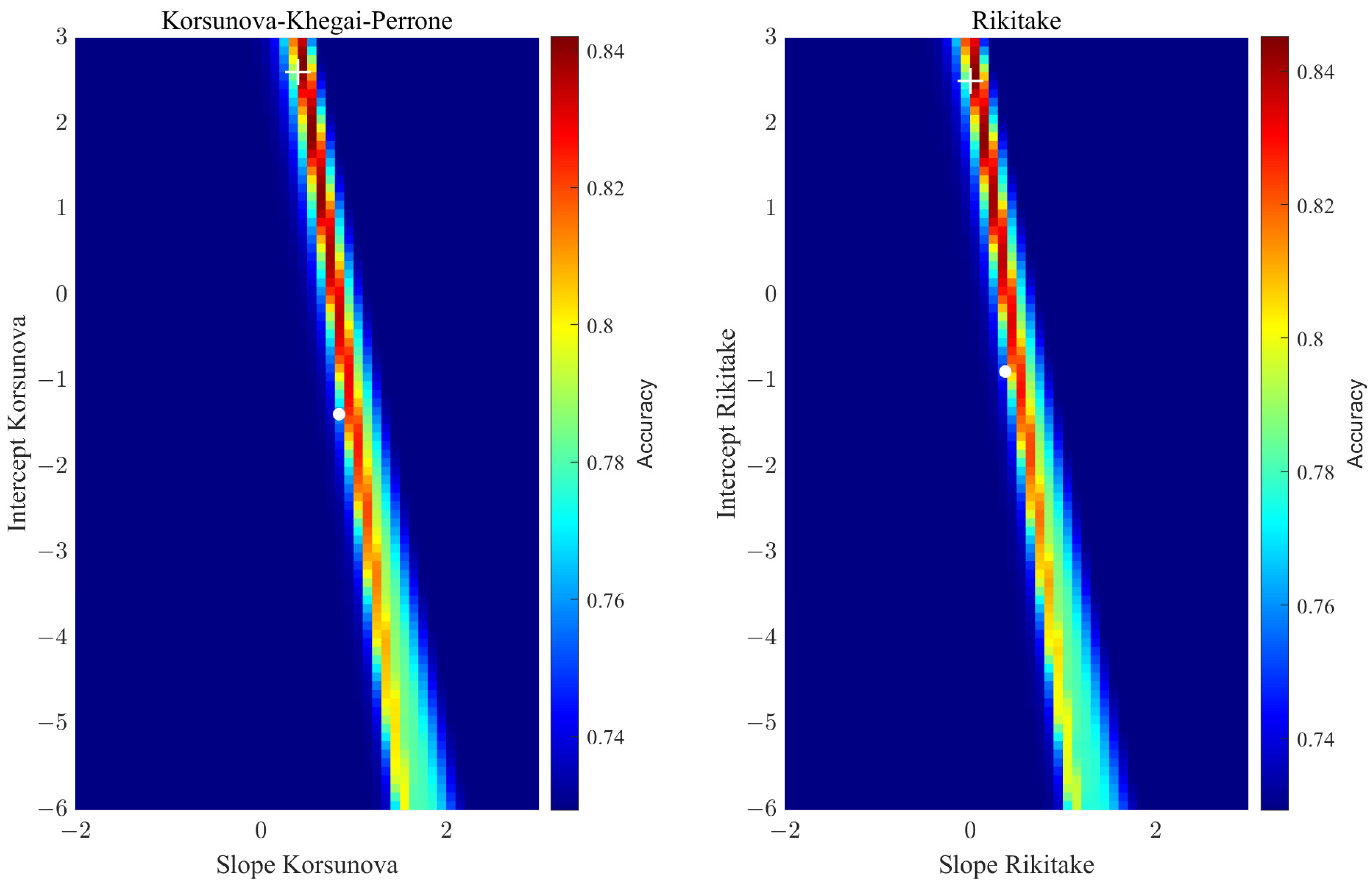
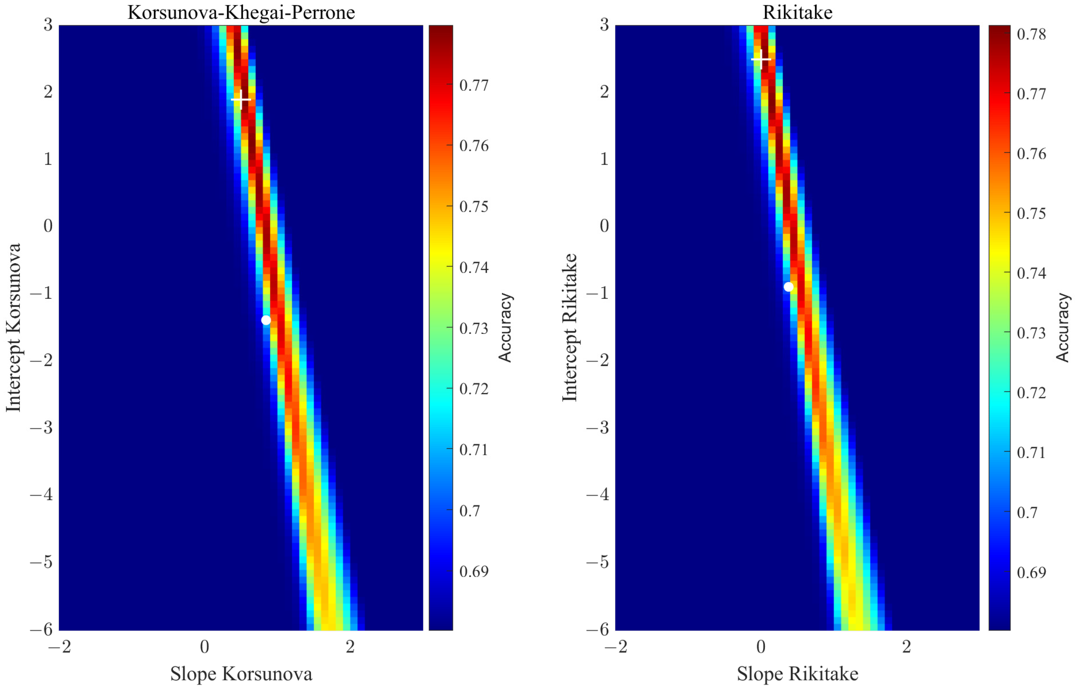
  • ak × M + bk; coefficients of the Korsunova–Khegai–Perrone relationship.
  • aR × M + bR; coefficients for Rikitake’s law.
In case the above estimations are equal within the tolerance “tol”, we associate the anomaly with the earthquake, while in the other case, we consider it a false alarm. In detail, we consider an anomaly possibly associated with an earthquake if:
  • |Log10(ΔT × R) – (ak × M + bk)| < tol for the Korsunova–Khegai–Perrone relationship.
  • |Log10(ΔT) – (aR × M + bR)| < tol for Rikitake’s law.
In this work, we also tested our result with original coefficients for the two laws. In particular, for “Korsunova-Khegai-Perrone”, the value is calculated as the mean of the ones provided for Italy in [40] and for Greece in [41] and equal to ak = 0.84434 and bk = −1.38636. For the Rikitake law, we selected the proposed coefficients for precursors of “quasi-1st kind” in the original paper [45] and equal to ar = 0.38 and br = −0.89.

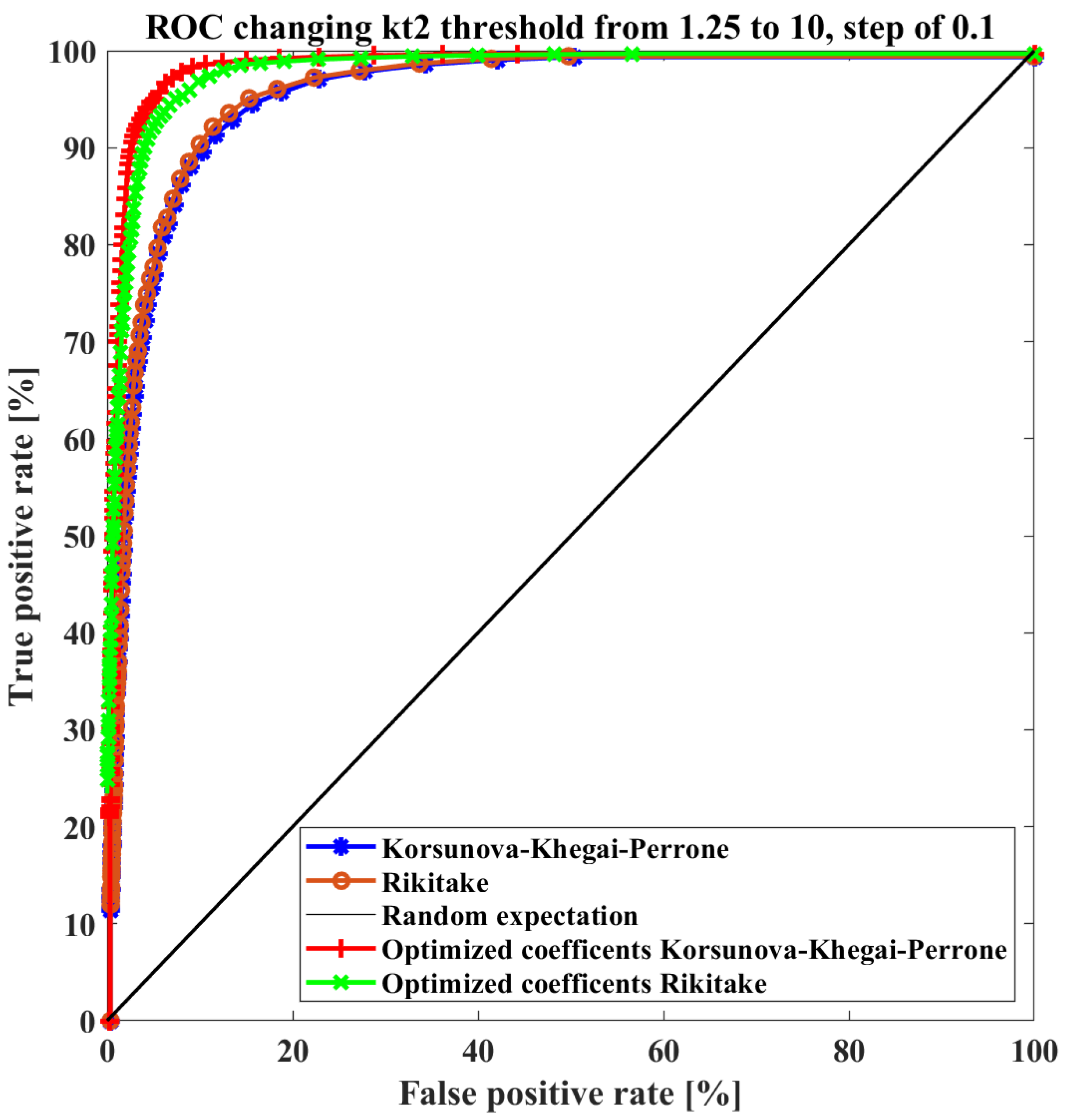
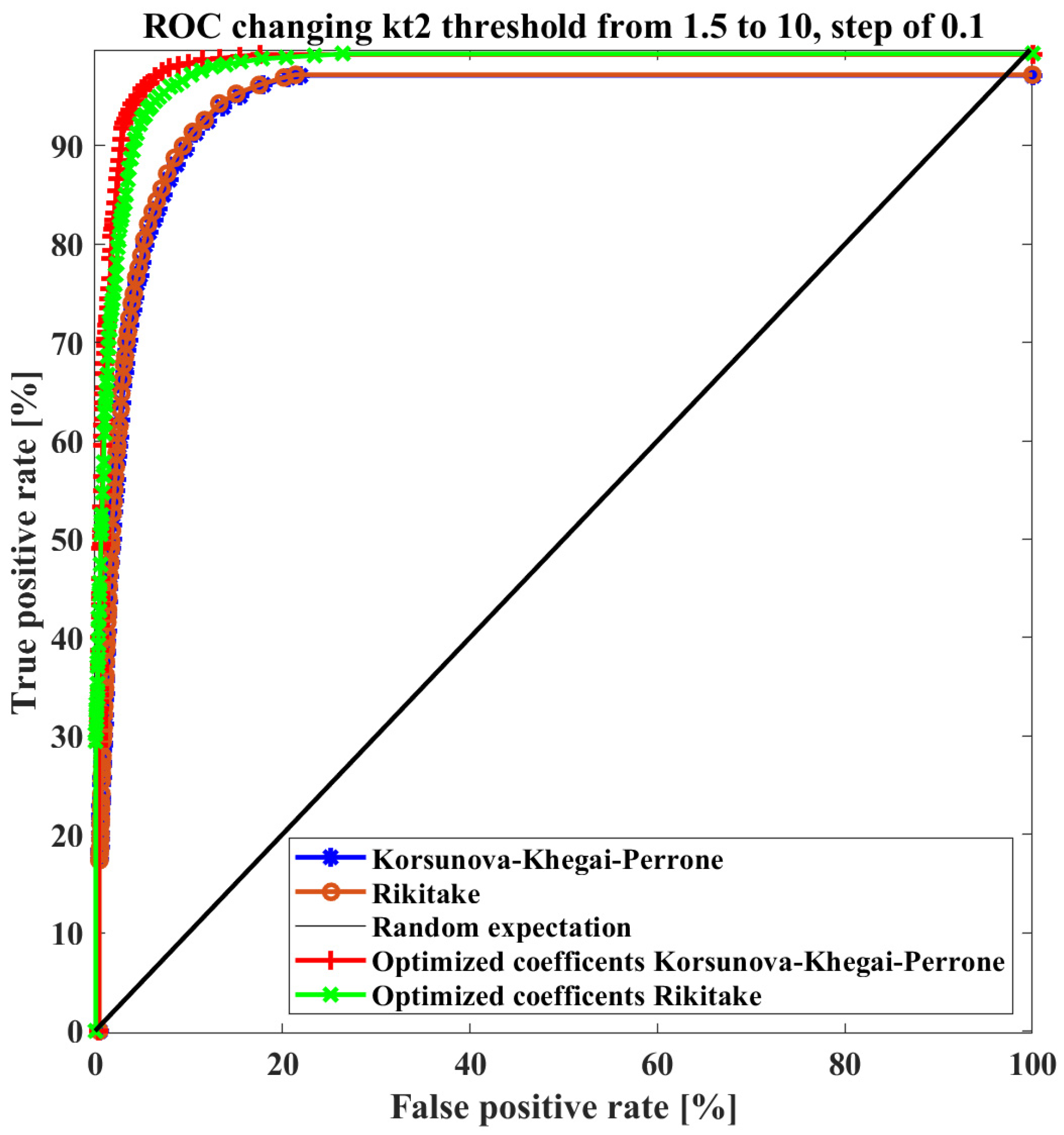
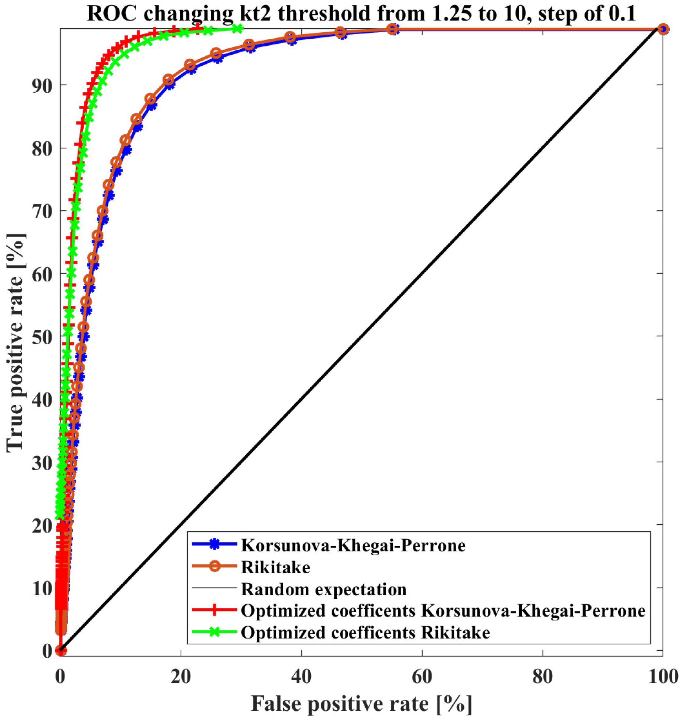
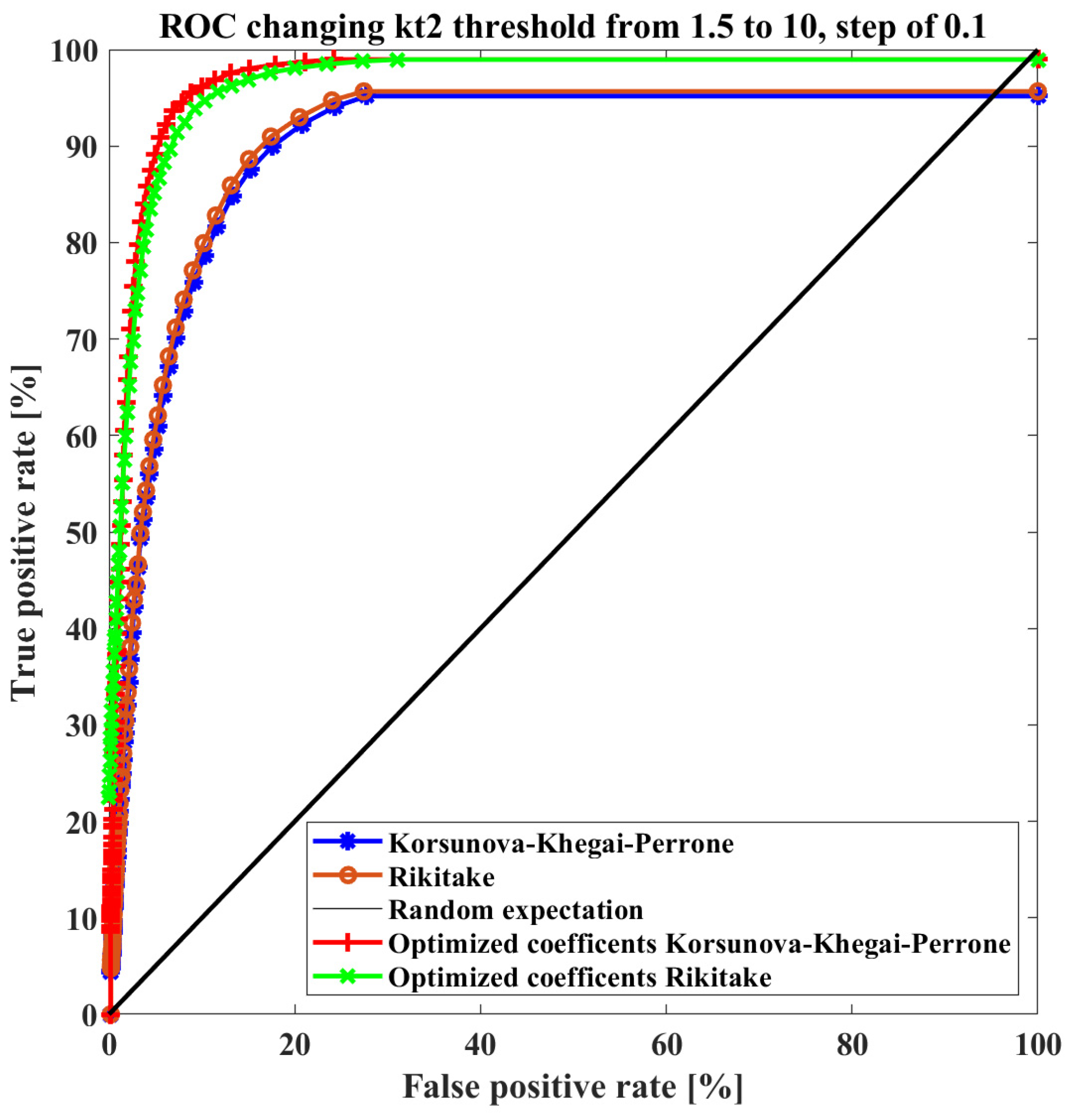
2.2.5. Assessment of Prediction Capability with Confusion Matrix and ROC Curves

To evaluate the prediction capability of the method, we used the classic confusion matrix approach defined by Fawcett [76] and widely used in earthquake prediction assessment together with receiving operating characteristic (ROC) graphs [77,78,79]. From the above proceeding, illustrated in Figure 3, we extract the true positives and the false positives; we still need to estimate the true negatives and the false negatives. Here we use as a reference the cells used for the background (and illustrated in Figure 1 as red or grey boxes) and the month as a time unit, and in particular, we remark:
  • A “true positive” (TP) is a cell with Ne anomalies associated with an incoming earthquake.
  • A “false positive” (FP) is a cell with Ne anomalies not associated with incoming earthquakes.
  • A “true negative” (TN) is a cell without Ne anomalies and without earthquakes.
  • A “false negative” (FN) is a cell without Ne anomalies but with one or more earthquakes.
From these definitions, we calculated the accuracy “Acc”:
A c c = T P + T N T P + F P + T N + F N
The last point of this work is to search for the best coefficients of the applied relationship for CSES-01 Ne satellite data correlated with M5.5+ shallow earthquakes. This task is an optimisation run, and it is performed searching for the maximum accuracy changing the intercept of the Korsunova–Khegai–Perrone or Rikitake relationships within the range [−6; 3] (step of calculus 0.1) and slope within the range [−2; 3] (step of calculus 0.1).

3. Results

In this section, we present our results, first in terms of ionosphere background characterisation and, second, possible association with the anomalies.

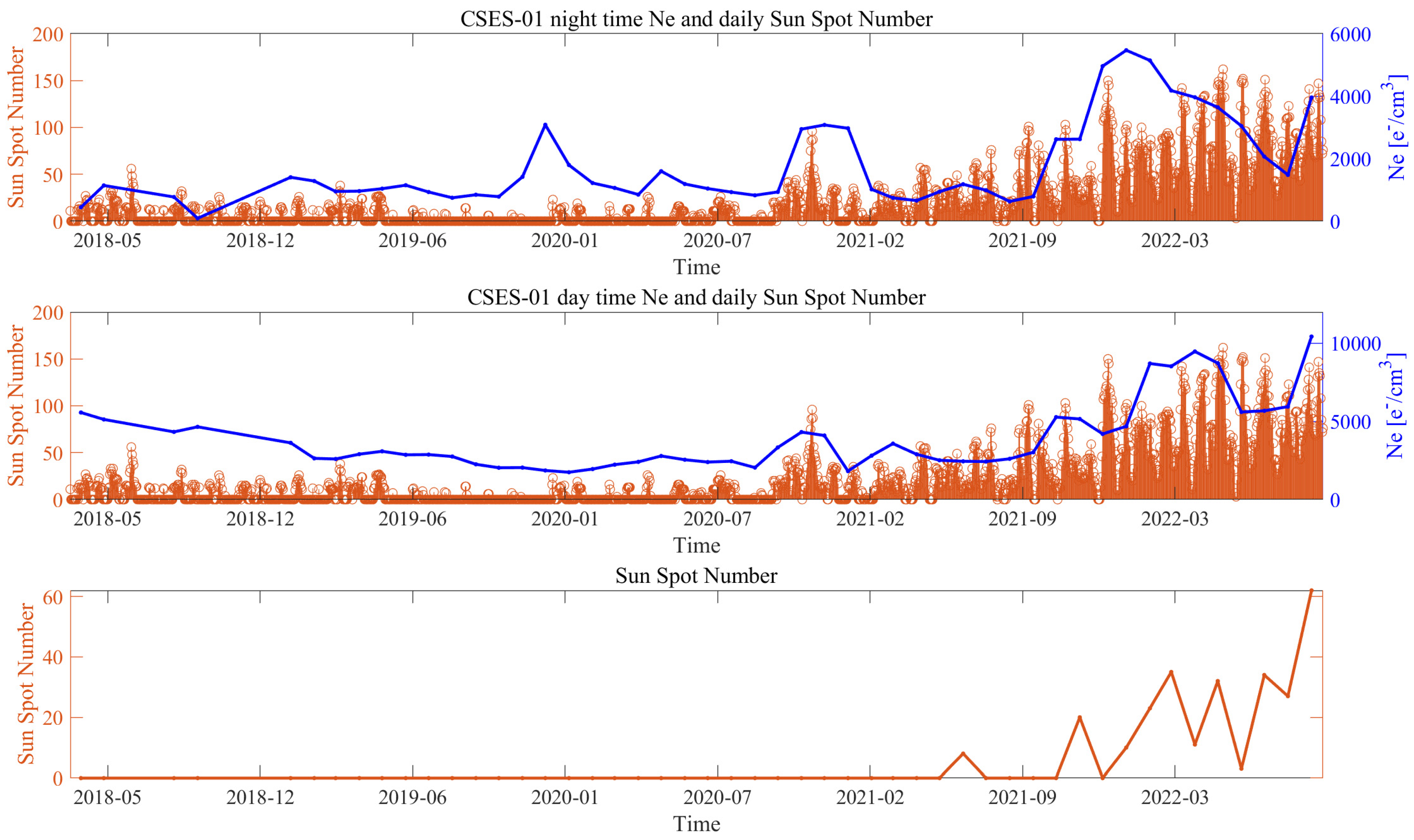
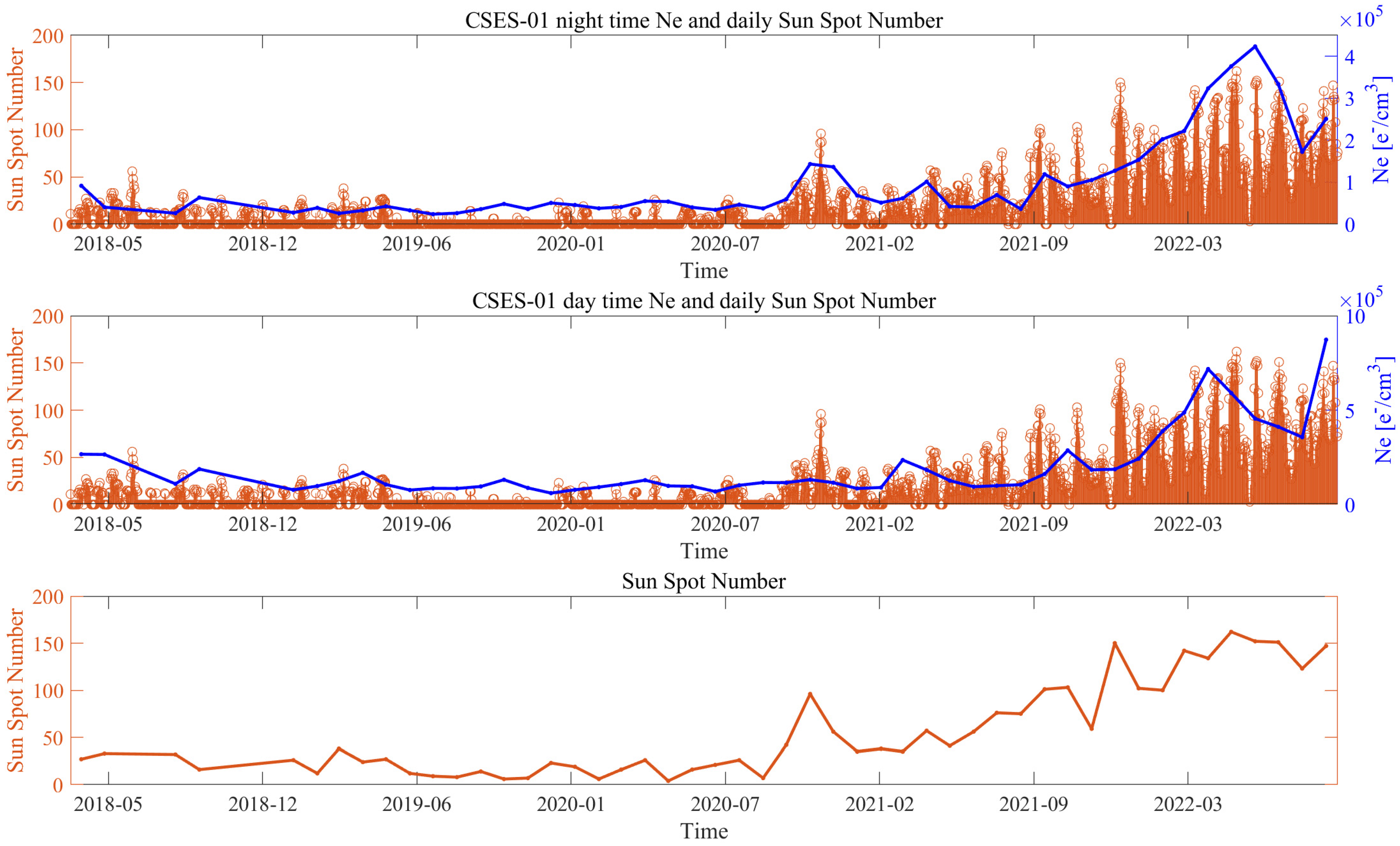
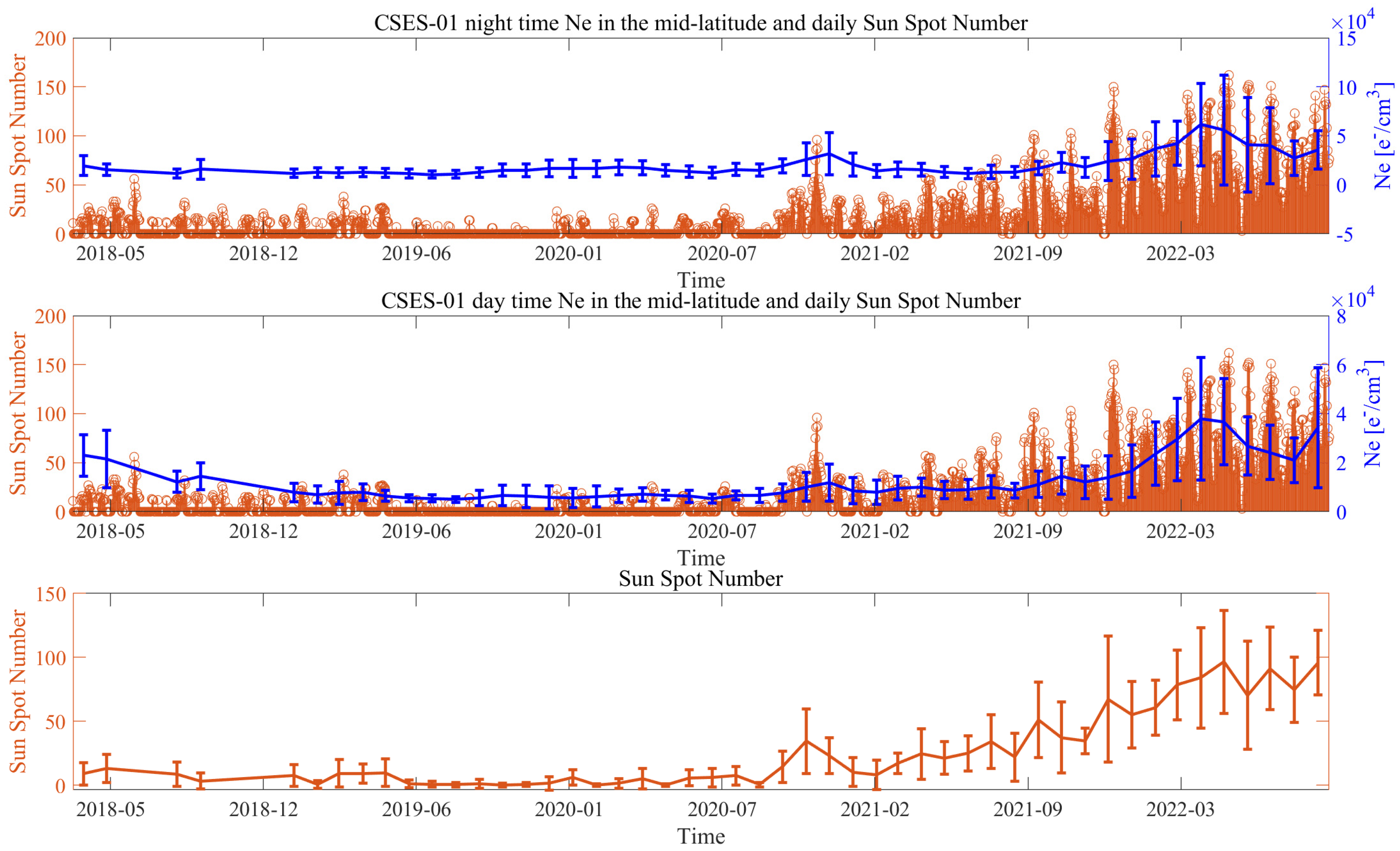
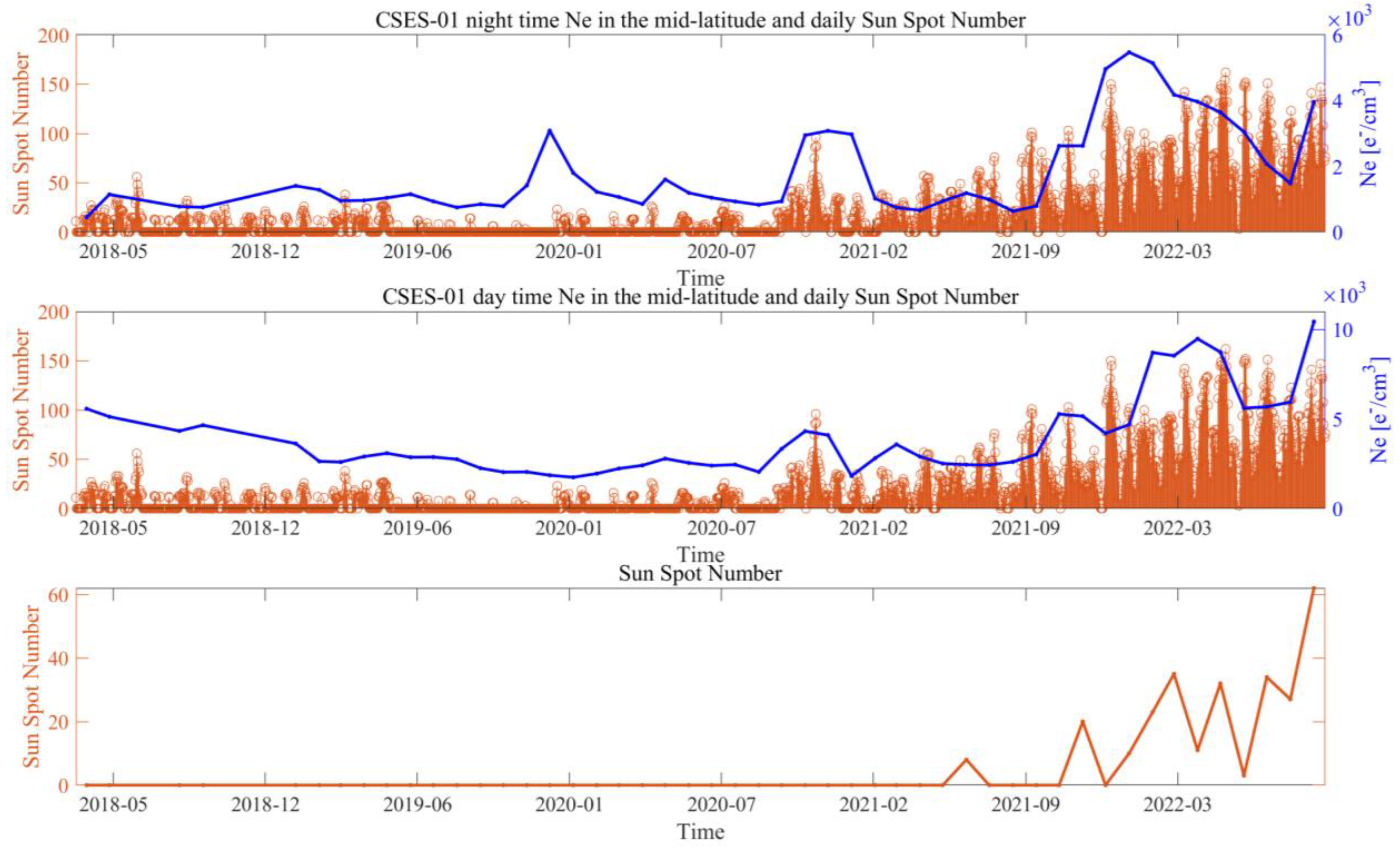
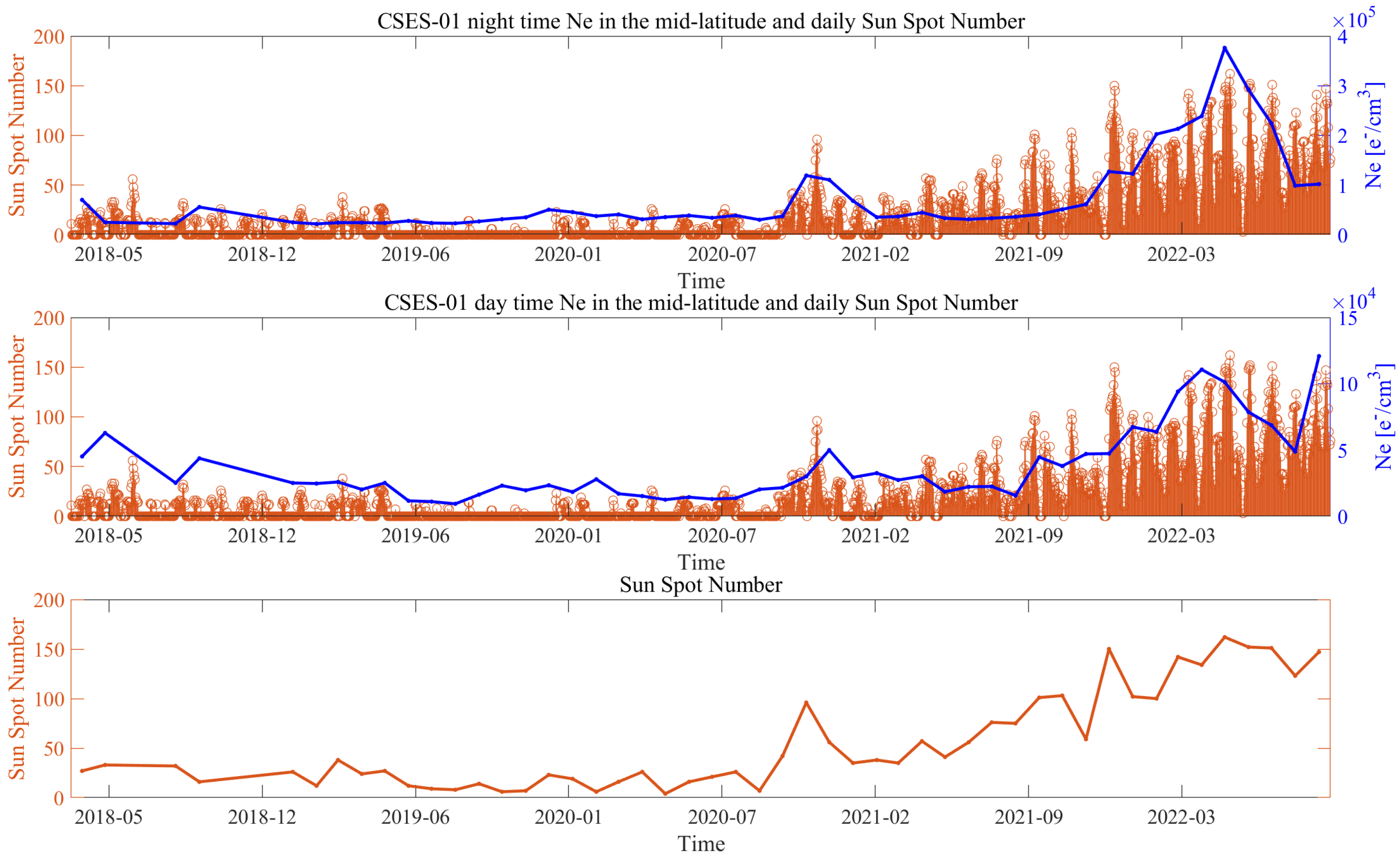
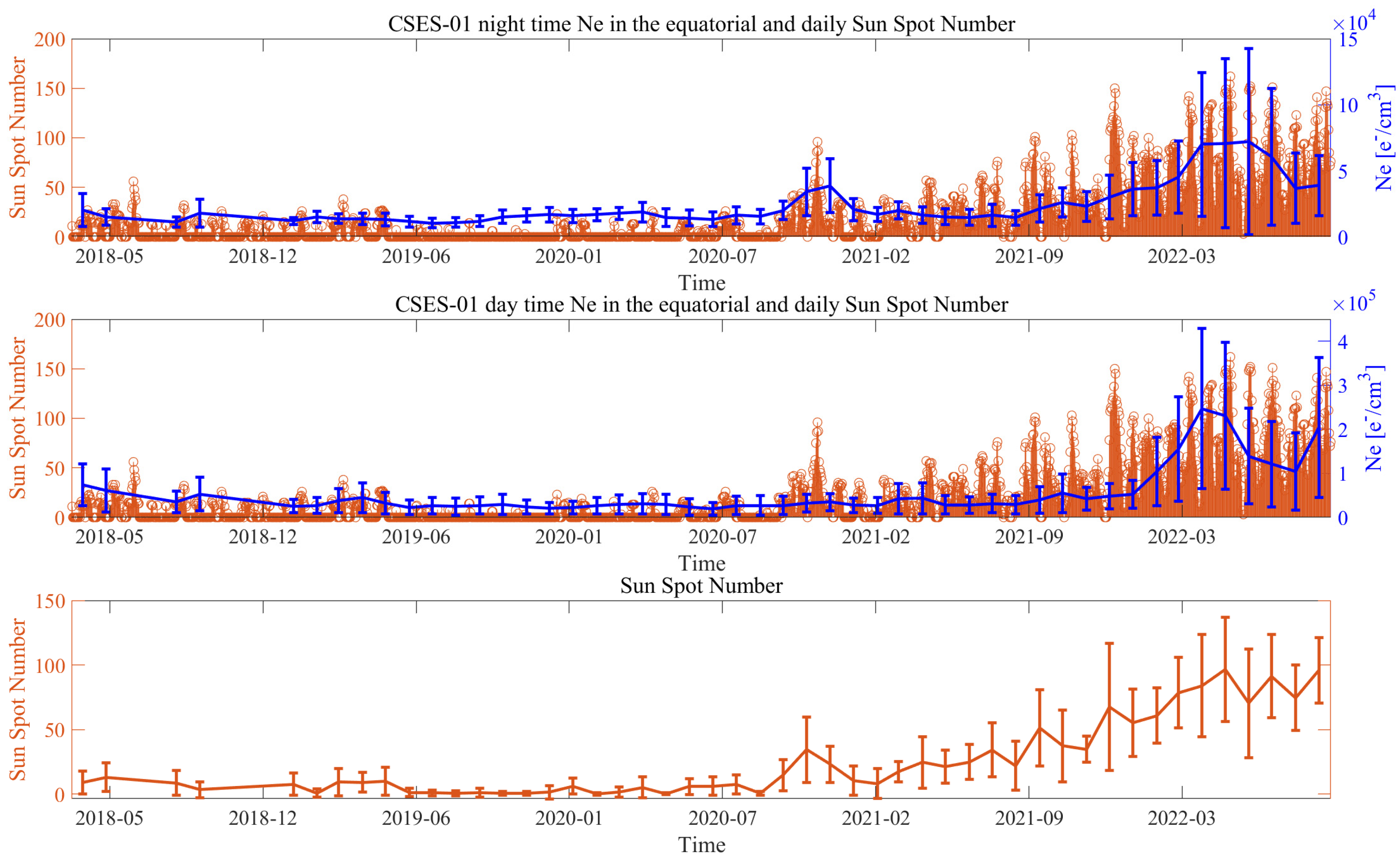
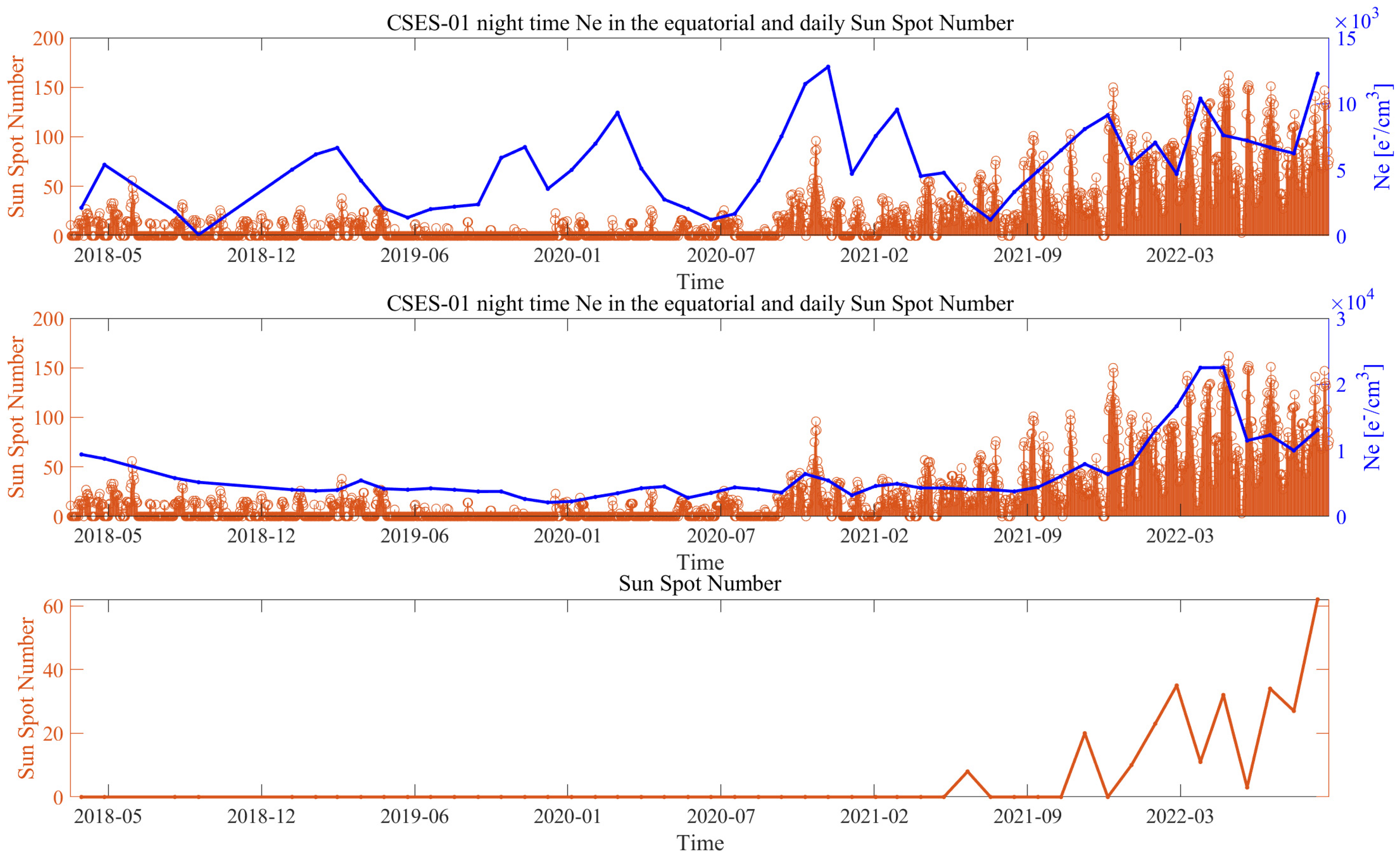
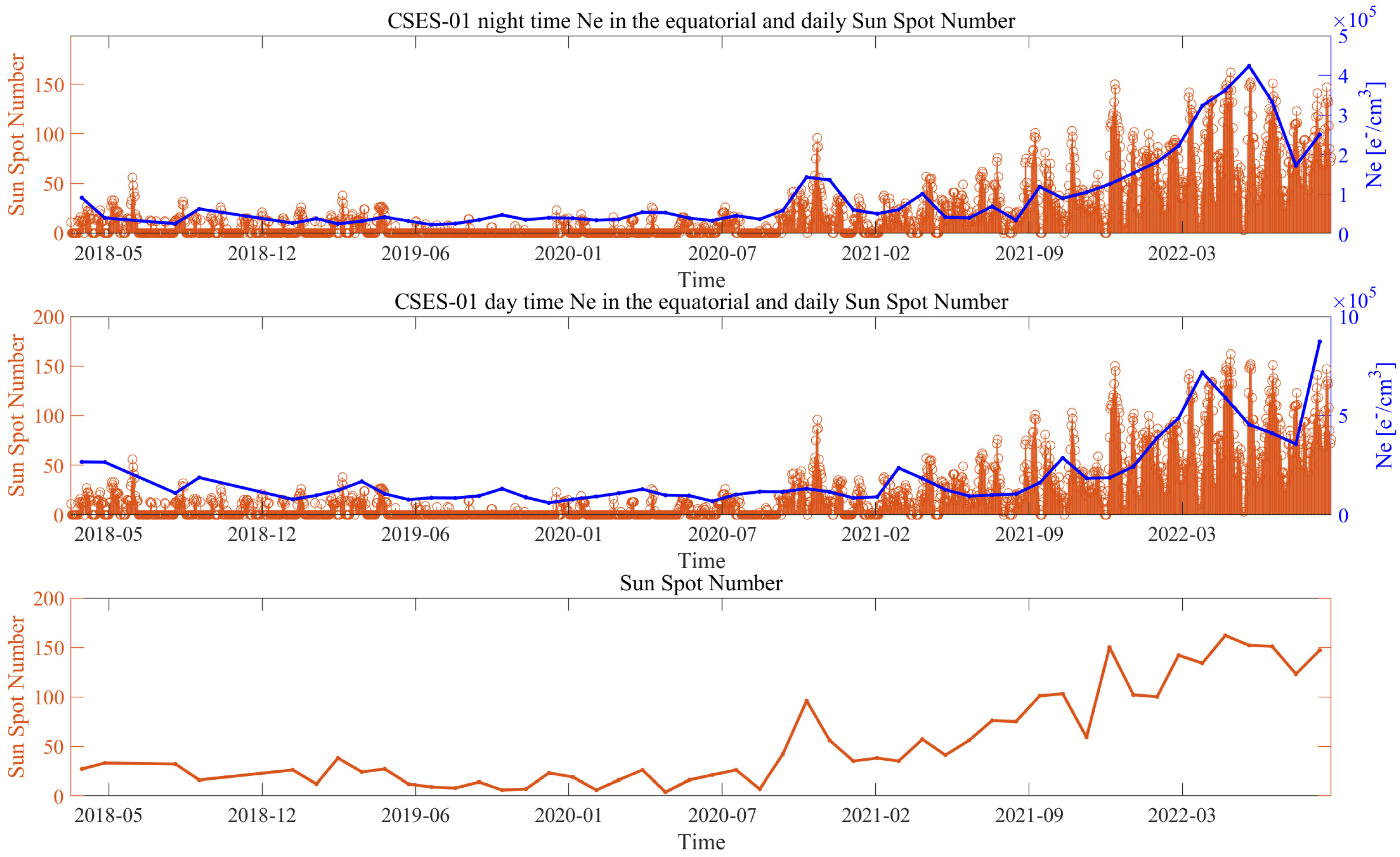
3.1. Ionospheric Background Satellite Ne Characterisation

3.1.1. Background for Night- and Daytime

The available CSES-01 electron density data have been used to prepare a monthly satellite background characterisation for the nighttime and daytime. Even though the first six months of CSES-01 were the commissioning phase (so the data are normally excluded for scientific purposes), we would include and compare with the standard operating satellite operational period. So, we analysed April, August, and September of 2018 and from January 2019 to September 2022 for a total of 48 months (4 years). Figure 4 reports the monthly median background values acquired in geomagnetic quiet conditions for nighttime. It is possible to note similar structures in the same season, for example, blobs of high electron density in the south of the Western Hemisphere (around South America) in January–March as well as in the south of the Eastern Hemisphere in June–August (or September). These structures seem to be reduced in the last investigated year (2022), probably as a consequence of the increase in solar activity, as further discussed in the following section.
Figure 5 shows the monthly median background values for daytime observations of the CSES-01 satellite. A clear activity of the ionosphere around the geomagnetic equator can be depicted in all the maps. This underlines the equatorial ionospheric anomaly (EIA) driven by solar irradiation. It is well present at 2 p.m. and close to the time of its maximum value. The absolute Ne values in the daytime are always higher compared with the nighttime median shown in Figure 4, as expected. In fact, the principal source of the ionisation is the Sun. Consequently, the part of the Earth facing the Sun experiences a higher level of electron density due to solar irradiation.
For the variations in electron density at night- and daytime as a function of the date, we refer to Section 3.1.2, and Appendix A, where the mean, standard deviation, minimum, and maximum CSES-01 Ne values are extracted.

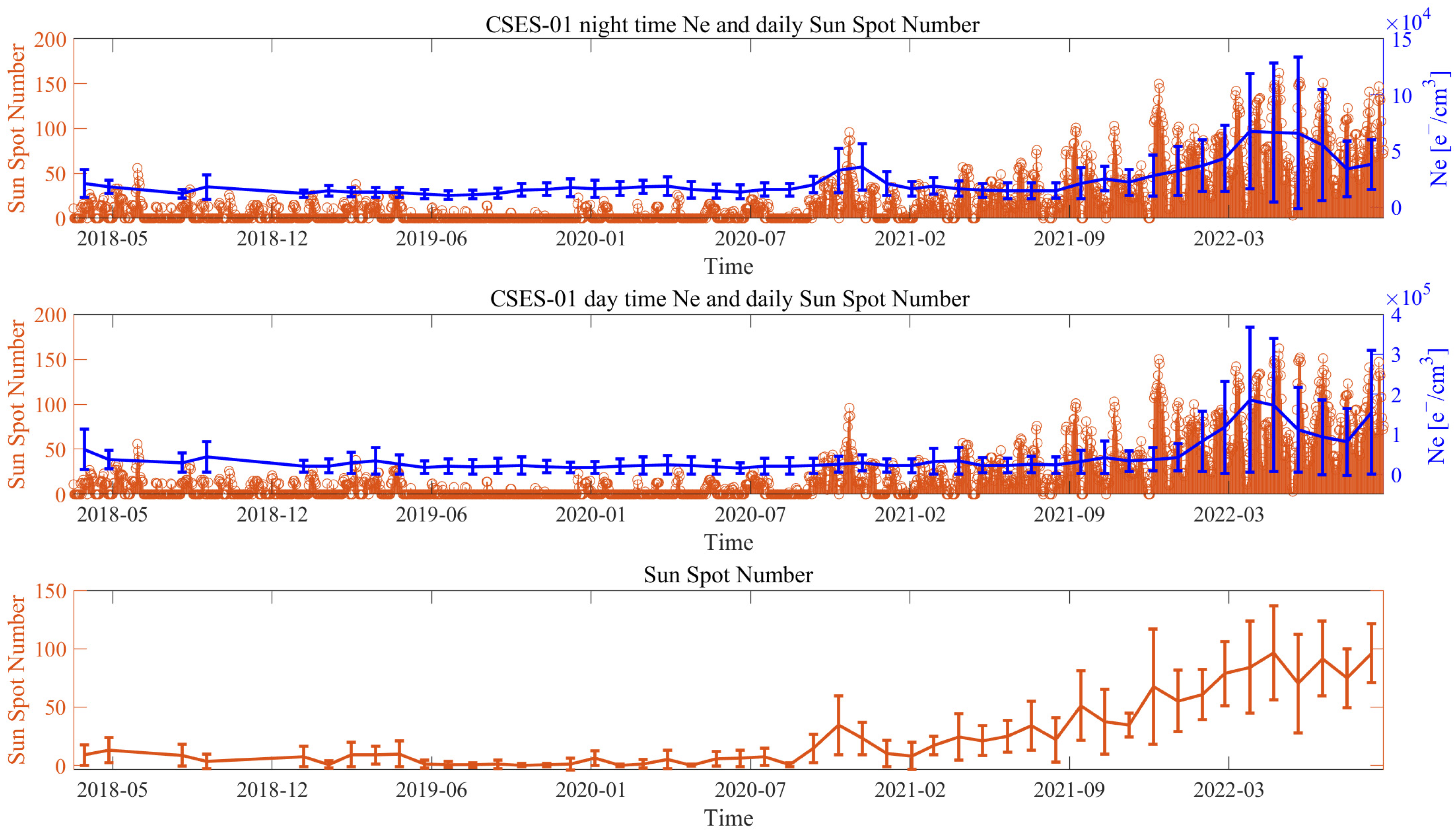
3.1.2. Comparison of the Ionospheric Background with Solar Activity

This section compares the backgrounds of ionospheric night- and daytime with solar activity. We retrieved the daily sunspot number as a parameter representative of solar activity. Sunspot number index has already been very well correlated with ionospheric status, for example, TEC [23,80]. The mean, standard deviation, minimum, and maximum values have been extracted for each background map and correlated with the same quantities of sunspot numbers. For Ne, the mean, standard deviation, and minimum and maximum values are computed over the available values in the map. For the sunspot number, the same quantities are computed over the daily values of the specific month under investigation. Figure 6 shows the mean value of CSES-01 electron density in each night and day monthly background as a function of time. The daily sunspot number is shown for comparison, and the mean of this quantity is also reported. Figure 7 and Figure 8 show the minimum and maximum CSES-01 background values calculated for each background. It is possible to note that there is a great agreement between the trends of electron density recorded by the CSES-01 satellite and solar activity. In 2018, only some tracks in the months of April, May, August, and September have been analysed due to the commissioning operations of the CSES-01 satellite. From 2019, all the months have been continuously analysed. In previous Figure 4 and Figure 5, the maps of May 2018 are not provided for very small amounts of data. In particular, in the last investigated year (i.e., 2022), solar activity increased due to approaching the maximum of the 25th solar cycle. Consequently, and as expected, the ionosphere increased its ionisation status. This is a measurement of the ionospheric activity and evidence that CSES-01 provides reliable and precious data to monitor the complex ionospheric environment. To further investigate the correspondence between the CSES-01 Ne and the sunspot number, we estimated the Pearson correlation coefficient “R” between the minimum, mean, and maximum CSES Ne and sunspot number for day- and nighttime. R coefficients for all the combinations are reported in Table 1. It is possible to note that the maximum correlation coefficient equal to 0.89 and 0.85 is obtained with the correlation of the maximum electron density value compared with the sunspot number’s mean value. The low correlation of the minimum sunspot number with electron density background values (except for maximum daytime CSES-01 Ne) is due to several zeros in the time series of sunspots, as there was at least one day each month without sunspots on the surface of the Sun before 2022. On the other side also, the maximum values of the sunspot number show a lower correlation with the electron density background values (except for the nighttime mean and maximum values). This can be due to the fact that we excluded the electron density samples acquired in disturbed geomagnetic time typically induced by high solar activity. However, the nighttime maximum values of CSES-01 Ne background are very well correlated (0.89) with the mean of the sunspot number. This could underline a delicate point regarding the study of the ionosphere, i.e., the ionosphere’s response to solar activity at nighttime, even during “apparently” geomagnetic quiet time.
Finally, the best correlation is that of the mean sunspot number with the maximum monthly median value recorded by CSES-01 both at night- and daytime.
We also provided a comparison of CSES-01 Ne in mid-latitude and equatorial regions. The specific time series are presented in Appendix A, while the correlation coefficients are reported in Table 1. The equatorial region is the one with the EIA crests during the daytime, but as we analysed only geomagnetic quiet time, some response of the ionosphere (in particular EIA) during the increase in solar activity could be lost in this study. In fact, previous studies investigated the relationship between EIA features and solar activity [81]. This could be explored in a future dedicated study, which includes the geomagnetically disturbed time (here excluded as the final goal is to investigate possible seismo-ionospheric disturbances). Finally, our result confirmed previous studies performed by Bilitza et al. [82] on the CHAMP and ionospheric model with a new satellite mission (i.e., CSES). Their paper shows a good agreement between the electron density in the top-side ionosphere and solar activity.

3.2. Correlation of CSES Ne Anomalies with Earthquakes

In this section, we extracted anomalies comparing Ne with the previously defined background that will be correlated with the shallow M5.5+ earthquakes shown in Figure 3. We will test two anomaly definitions and two possible relationships of ionospheric anomalies and earthquakes, which we call the “Korsunova-Khegai-Perrone” and “Rikitake” laws. We should underline that these are extensions of these relationships to the data we are analysing and not the original method developed on a different set of parameters for other instruments and conditions. We also present the results in this section for mid-latitude and equatorial regions separately. This permits testing the methods in these two regions, which present very different ionospheric conditions. In particular, the equatorial region is more active, and some other research has been excluded. However, previous studies by Parrot et al. [83], based on the DEMETER satellite, proposed that the electron density profile in the equatorial region is enhanced before the earthquake. For this reason, we found it worth also investigating this region. Still, to avoid a possible “contamination” of the results, we separate the calculations in the equatorial region from those for the mid-latitude one.

3.2.1. Results Testing the Mid-Latitude Anomalies Defined over Median and IQR

Figure 9 presents the accuracy obtained using the anomalies defined as the values that are greater than the median plus 1.25 times (kt2) the interquartile range for mid-latitude regions for the “Korsunova-Khegai-Perrone” and “Rikitake” laws. In these analyses, we considered a fixed tolerance associating the anomaly to the earthquake with the law being tested equal to 0.606, which is the semi-maximum dispersion of the laws provided by Perrone et al. [40,41] for Italy and Greece. The best coefficients (marked with a white cross in Figure 9) are ak = 0.4, bk = 2.6, ar = 0.0, and br = 2.5 and the corresponding confusion matrix is provided in Table 2.
After extracting the coefficients with maximum accuracy (underlined with a white cross in Figure 9), we constructed the ROC curves, changing the kt2 threshold to define the anomalies, which we show in Figure 10. We also plot the ROC curves using the original coefficients (mentioned above) as a reference.

3.2.2. Results Testing the Mid-Latitude Anomalies Defined as “Outlier”

Here, we present the results extracting the anomaly defined using the outlier definition (i.e., anomaly > Q3 + kt2 × IQR) and investigating the mid-latitude regions (northern and southern ones). In particular, firstly, we selected the anomaly using the mild outlier definition (kt2 = 1.5), and we searched for the maximum accuracy as a function of slope and intercept for the “Korsunova-Khegai-Perrone” and “Rikitake” laws, as reported in Figure 11.
The best coefficients (marked with a white cross in Figure 11) are ak = 0.4, bk = 2.6, ar = 0.0, and br = 2.5; the corresponding confusion matrix is shown in Table 3 and the ROC curves shown in Figure 12 are calculated using them. As in the previous case, the optimised coefficients show better prediction performances than the original coefficients. In addition, the “Korsunova-Khegai-Perrone” law provides better predictability than Rikitake, due probably to one more parameter in the model, i.e., the distance of the anomaly from the earthquake.

3.2.3. Results Testing the Equatorial Anomalies Defined over Median and IQR

In analogy with previous results, Figure 13 presents the variation in the accuracy as a function of different slopes and intercepts for equatorial region anomalies defined with respect to the median and interquartile range (kt2 = 1.25). The best coefficients (marked with a white cross in Figure 13) are ak = 0.5, bk = 1.9, ar = 0.0, and br = 2.5 and the corresponding confusion matrix is provided in Table 4. Figure 14 reports the corresponding ROC curve for these best parameters.

3.2.4. Results Testing the Equatorial Anomalies Defined as “outlier”

Figure 15 shows the optimisation of the “Korsunova-Khegai-Perrone” and “Rikitake” laws for the equatorial region with the mild outlier definition of CSES-01 Ne anomalies. The best coefficients (marked with a white cross in Figure 15) are ak = 0.5, bk = 1.9, ar = 0.0, and br = 2.5 and the corresponding confusion matrix is provided in Table 5. Figure 16 reports the corresponding ROC graph made with the previously identified best coefficients.

4. Discussion

In this work, we constructed a monthly ionospheric satellite background using the CSES-01 Ne data similar to that of Sabbagh et al. [9] for the CHAMP and Swarm satellites. Here, we used cells of 5° of longitude, 5° of latitude, and monthly data acquired in geomagnetic quiet conditions in mid-latitude and equatorial regions. Two distinct backgrounds for night- (~2 a.m.) and daytime (~2 p.m.) were constructed and represented in Figure 4 and Figure 5, respectively.
The obtained background was compared with the sunspot number, finding excellent agreement between the trends shown by the Pearson correlation coefficient equal to 0.89 for the night and 0.85 for the day of maximum Ne monthly background values in the whole region and mean sunspot numbers.
Finally, we tested two approaches to the possible correlation of the anomalies with the earthquakes, which we called the “Korsunova-Khegai-Perrone” and “Rikitake” laws. We first used the original coefficients proposed by other papers that introduced these laws. Despite this, they retrieved the coefficients for different anomaly types, different definitions of an anomaly, and different instruments. We optimised the best slope and intercept for the two laws separately for equatorial and mid-latitude regions and with two anomaly definitions used in this paper. Table 6 summarises the best coefficients obtained in all the explored conditions and regions together with the obtained accuracy, from 58.0% up to 84.5%. Accuracy greater than 50% tends to support a statistical correlation between the ionospheric anomalies and earthquake occurrence. In addition, the number of earthquakes preceded by anomalies is reported, including their percentage with respect to total analysed seismic events. The total analysed earthquakes correspond to 328 for the mid-latitude regions and 1019 for the equatorial region.
Looking at the best combinations in Table 6, it is worth noting that the best coefficients are independent of the specific method for selecting the anomaly. Nevertheless, the process based on the formal definition of an outlier (Q3 and IQR) provides higher accuracy than the one based on median and IQR. The accuracy in the equatorial region with the median and interquartile range anomaly definition provides a poor value of about 58%. This could reflect that the ionosphere in this region has highly intrinsic variability not related to earthquakes. Consequently, the definition of anomalies based on median and interquartile range resulted in too many false alarms, i.e., anomalies due to normal variability in the ionosphere in this region. However, using the mild outlier anomaly definition, an accuracy of 78% or higher can be obtained, confirming that also in the equatorial region, there are increases possibly due to seismic activity, but it is necessary to have a stronger definition of an anomaly to depict them correctly. For the Rikitake law, all the approaches in equatorial and mid-latitude regions provide a null best slope. This would mean that the anticipation time of the CSES-01 Ne ionospheric anomaly extracted in this paper would not depend on earthquake magnitude, and it is about 10.5 months. This time could appear large, but it is fully within the results previously obtained for the Swarm Ne satellite by De Santis et al. [43] and Marchetti et al. [44]. Following our results for Rikitake’s law, it seems that the dependence on the magnitude identified for the “Korsunova-Khegai-Perrone” relies only on the distance of the anomaly from the earthquake as the logarithm of the product of the distance in space and time can be decomposed in the sum of logarithms: log 10 T × R = log 10 T + log 10 R . The null slope is a surprising result, but it could explain in a different way parts of the work proposed by De Santis et al. [43] and Marchetti et al. [44]. In fact, in both papers, based on 4.7 and 8 years of Swarm satellite data correlated with M5.5+ shallow earthquakes (the same catalogue used in this paper in the same analysed time), the authors identified a very good dependence of anticipation time of magnetic anomalies with earthquake magnitude, but less effective results using electron density anomalies. In particular, De Santis et al. [43] tried to propose a “Rikitake” relationship for Ne using a manual selection of the maximum concentration of anomalies, and Marchetti et al. [44] used the automatically extracted concentrations. Still, two used points over five presented “ambiguous” values not in agreement with the Rikitake law. The results obtained here could explain why the Rikitake law may not apply to some electron density anomalies retrieved by satellite data. Despite this, we underlined that the types of extracted anomalies in [43,44] are variations around the baseline of the signal (relative anomalies). At the same time, in this paper, we used an absolute increase in electron density compared to the designed background. Further investigations are consequently required. Another point is taken from He and Heki [20], who also proposed the Rikitake law for electron density (or TEC) satellite values, but with a very much shorter anticipation time (in the range from 20 min to 1 h before the earthquake). The anticipation times investigated in this paper and [57,58] are on a totally different scale of days/months. This suggests that the Rikitake law may still apply but to another kind of ionospheric satellite anomalies on a shorter precursor time.
In addition, comparing the equatorial with mid-latitude regions, the results are similar, showing that the ionosphere seems to be affected in the same manner inside the whole investigated region (50° S ~ 50° N).
We noted that in all the investigated combinations for the two laws, regions (mid-latitude or equatorial one), and anomaly definitions in Figure 9, Figure 11, Figure 13 and Figure 15, there is a combination of parameters defining an orange-red region which is good and with similar accuracy. This means that combinations other than the “best” bring similar results. However, it is clear that not all combinations are equally good. This is a delicate point for the Rikitake law, in that shifting to another combination means having a slope different from zero.
Comparing Figure 9, Figure 11, Figure 13 and Figure 15, we noted that in all cases, the coefficients proposed by the previous papers we refer to (Perrone et al. [54,55] and Rikitake [45]—marked by white dots) fall in the “good accuracy” region of our investigation, but the present study extracted higher maximum accuracy.

5. Conclusions

Finally, our main conclusions can be summarised in the following points:
  • CSES-01 Ne data are reliable measurements of the status of the ionosphere. In fact, the observations permitted constructing an ionospheric background highly in agreement with solar activity (R = 0.85 for daytime and R = 0.89 for nighttime).
  • Increases in CSES-01 Ne with respect to the background seem statistically related to the seismic activity of shallow M5.5+ worldwide earthquakes as supported by the accuracy higher of 50% (≥78% for the mild outlier anomaly definition) for all the explored cases in this paper. This further supports statistically the existence of ionospheric disturbances before the earthquakes.
  • The anticipation time of the identified CSES-01 Ne ionospheric anomalies seems to not depend on earthquake magnitude due to the null best coefficient obtained for the “Rikitake” law. Despite this, the distance of the ionospheric anomaly from the earthquake seems to increase with earthquake magnitude both in equatorial and mid-latitude regions, as suggested by positive slopes (0.4 and 0.5) estimated for the “Korsunova-Khegai-Perrone” law.
We would underline some limitations of the present work that future studies and satellite and ground experiments could try to address:
  • This study is limited to one parameter (Ne), one type of anomaly (increase in electron density) and one satellite. Future studies can try to integrate multiple parameters and include other types of anomalies.
  • The investigation time before the earthquakes depends on the same earthquake time. For example, an earthquake in 2022 has more than three years of CSES data, while an earthquake in 2019 is only several months. Extension of CSES-01 and integration with at least a second CSES satellite would permit a larger dataset with more time coverage.
  • We preferred to investigate the anomalies inside Dobrovolsky’s area as the earthquake preparation zone, as it is physically related to the seismic event, but other areas (physically related or not and even fixed) may be used.
  • We limited our study to the anticipation time and distance of the anomalies with respect to the incoming earthquake. Still, it is also worth investigating the intensity of the anomaly, its duration/extension in space (on the satellite, they are intrinsically related), direction with respect to the epicentre as well as the eventual influence of the earthquake focal mechanism, location of the earthquake (sea/land or Northern/Southern Hemispheres), etc.
In addition, future investigations are required to better understand the mechanisms of lithosphere, atmosphere, and ionosphere coupling (LAIC), which can produce the identified anomaly. The seismo-induced disturbances in the ionosphere can be a direct electromagnetic effect, as proposed by Molchan and Hayakawa [84], or a chain of physical–chemical phenomena, as suggested by Pulinets and Ouzounov [54]. In conclusion, the China Seismo Electromagnetic Satellite (CSES-01) is providing precious observations to better understand the possible effect of earthquakes in the ionosphere before their occurrence.

Author Contributions

Conceptualisation, D.M.; methodology, D.M. and D.S.; software, D.M. and W.C.; validation, R.Y., D.S., Y.Z. and Z.Z.; formal analysis, investigation and visualisation, D.M. and W.C.; resources, D.M. and K.Z.; data curation, R.Y., D.M. and W.C.; writing—original draft preparation, D.M.; writing—review and editing, D.M., D.S., W.C., Z.Z., X.S., Y.C., M.F., S.W., T.W., D.Z., H.Z. and Y.Z.; supervision, project administration, funding acquisition, D.M. and K.Z. All authors have read and agreed to the published version of the manuscript.

Funding

This research was funded by the National Natural Science Foundation of China (grant numbers: 41974084 and 42374087); the China Postdoctoral Science Foundation (grant number 2021M691190) and the International Space Science Institute (grant numbers: International Team 553 and International Team 23-583).

Institutional Review Board Statement

Not applicable.

Informed Consent Statement

Not applicable.

Data Availability Statement

Electron density measurements from the CSES-01 satellite are freely available from the web portal www.leos.ac.cn (last accessed on 7 August 2023) upon registration and formal approval and they are maintained by the China National Space Administration (CNSA). The global earthquake catalogue is freely available from https://earthquake.usgs.gov/earthquakes (last accessed on 7 August 2023) maintained by the USGS (United States Geological Survey). Sunspot data were retrieved from the World Data Center (WDC) SILSO, Royal Observatory of Belgium, Brussels (https://www.sidc.be/SILSO/home, last accessed on 14 August 2023).

Acknowledgments

A special acknowledgement is for Loredana Perrone, who provided the basic ideas and knowledge to develop this study. The authors acknowledge ISSI/ISSI-BJ for supporting the International Team 553 “CSES and Swarm Investigation of the Generation Mechanisms of Low Latitude Pi2 Waves” led by Essam Ghamry and Zeren Zhima, and International Team 23-583 “Investigation of the Lithosphere Atmosphere Ionosphere Coupling (LAIC) Mechanism before the Natural Hazards” led by Dedalo Marchetti and Essam Ghamry. We acknowledge Angelo De Santis, Xiaodan He, Saioa Arquero Campuzano, Gianfranco Cianchini, Domenico Di Mauro, Martina Orlando, Alessandro Piscini, Maurizio Soldani, Jiami Wen, and Zining Yu for their participation in some scientific discussions of this work.

Conflicts of Interest

The authors declare no conflict of interest. The funders had no role in the design of the study; in the collection, analyses, or interpretation of data; in the writing of the manuscript; or in the decision to publish the results.

Appendix A

Comparison of CSES-01 Ne Background in Mid-Latitude and Equatorial Regions with Solar Activity

This appendix provides the same figures as the main manuscript (Figure 6, Figure 7 and Figure 8) but presented separately for mid-latitude and equatorial regions. In particular, Figure A1 shows the mean and standard deviations of CSES-Ne in mid-latitude regions graphically compared with daily sunspot numbers. In an analogous way, Figure A2 and Figure A3 show the minimum and maximum monthly values for the same time series. Figure A4, Figure A5 and Figure A6 report the mean (including standard deviation), minimum, and maximum of CSES-01 Ne, respectively, for the equatorial regions.
Figure A1. Time series of the mean electron density values in mid-latitude regions compared with the sunspot solar activity for night- and daytime backgrounds. The standard deviation of each quantity is shown as error bars. Daily values of the sunspot number index are shown together with the Ne values for comparison.
Atmosphere 14 01527 g0a1
Figure A2. Time series of the minimum electron density values in mid-latitude regions compared with the sunspot solar activity for night- and daytime backgrounds. Daily values of the sunspot number index are shown together with the Ne values for comparison.
Atmosphere 14 01527 g0a2
Figure A3. Time series of the electron density maximum values in mid-latitude regions compared with the sunspot solar activity for night- and daytime backgrounds. Daily values of the sunspot number index are shown together with the Ne values for comparison.
Atmosphere 14 01527 g0a3
Figure A4. Time series of the mean electron density values in equatorial regions compared with the sunspot solar activity for night- and daytime backgrounds. The standard deviation of each quantity is shown as error bars. Daily values of the sunspot number index are shown together with the Ne values for comparison.
Atmosphere 14 01527 g0a4
Figure A5. Time series of the minimum electron density values in equatorial regions compared with the sunspot solar activity for night- and daytime backgrounds. Daily values of the sunspot number index are shown together with the Ne values for comparison.
Atmosphere 14 01527 g0a5
Figure A6. Time series of the electron density maximum values in equatorial regions compared with the sunspot solar activity for night- and daytime backgrounds. Daily values of the sunspot number index are shown together with the Ne values for comparison.
Atmosphere 14 01527 g0a6

Appendix B

List of Parameters

In this appendix, we provide a list (in Table A1) of the parameters used in our method and their meaning or implications for the analysis.
Table A1. List of the parameters used in this study.
ParameterLong NameNotes on the Parameter and Its Result Implications
kt1Threshold to pre-select a dataset for anomaly extractionThis parameter does not have direct implications for the final results, but it permits us to reduce the original dataset when we search for anomalies in order to improve the computational efficiency
kt2Threshold to define the anomalyThis parameter is the threshold to define an anomaly. Higher kt2 implies the selection of fewer anomalies and in statistical distribution, it means selecting values on the positive tail of the distribution.
akSlope of the “Korsunova-Khegai-Perrone” lawThis parameter is set to ak = 0.844 or optimised on the real data, selecting maximum accuracy.
bkIntercept of the “Korsunova-Khegai-Perrone” lawThis parameter is set to bk = −1.386 or optimised on the real data, selecting maximum accuracy.
aRSlope of the “Rikitake” lawThis parameter is set to aR = 0.38 or optimised on the real data, selecting maximum accuracy.
bRIntercept of the “Rikitake” lawThis parameter is set to bR = −0.89 or optimised on the real data, selecting maximum accuracy.
ΔTAnticipation timeAnticipation time in days of a CSES-01 Ne anomaly with respect to a future earthquake
RDistanceDistance of an anomaly from the epicentre in km

References

  1. Hulburt, E.O. Ionization in the Upper Atmosphere of the Earth. Phys. Rev. 1928, 31, 1018–1037. [Google Scholar] [CrossRef]
  2. Briand, C.; Clilverd, M.; Inturi, S.; Cecconi, B. Role of Hard X-ray Emission in Ionospheric D-Layer Disturbances during Solar Flares. Earth Planets Space 2022, 74, 41. [Google Scholar] [CrossRef]
  3. Marconi, G. Radio Telegraphy. J. Am. Inst. Electr. Eng. 1922, 41, 561–570. [Google Scholar] [CrossRef]
  4. Piggott, W.R.; Rawer, K. 1913—U.R.S.I. Handbook of Ionogram Interpretation and Reduction. 1978. Available online: https://repository.library.noaa.gov/view/noaa/10404 (accessed on 1 October 2023).
  5. Huang, X.; Reinisch, B.W. Vertical Electron Content from Ionograms in Real Time. Radio Sci. 2001, 36, 335–342. [Google Scholar] [CrossRef]
  6. Scotto, C.; Sabbagh, D. The Accuracy of Real-Time hmF2 Estimation from Ionosondes. Remote Sens. 2020, 12, 2671. [Google Scholar] [CrossRef]
  7. McNamara, L.F.; Cooke, D.L.; Valladares, C.E.; Reinisch, B.W. Comparison of CHAMP and Digisonde Plasma Frequencies at Jicamarca, Peru. Radio Sci. 2007, 42, 1–14. [Google Scholar] [CrossRef]
  8. Merlino, R.L. Understanding Langmuir Probe Current-Voltage Characteristics. Am. J. Phys. 2007, 75, 1078–1085. [Google Scholar] [CrossRef]
  9. Sabbagh, D.; Ippolito, A.; Marchetti, D.; Perrone, L.; De Santis, A.; Campuzano, S.A.; Cianchini, G.; Piscini, A. Satellite-Based Electron Density Background Definition at Mid-Latitudes and Comparison with IRI-2016 Model under Different Solar Conditions. Adv. Space Res. 2023, 72, 1183–1195. [Google Scholar] [CrossRef]
  10. Chen, H.; Han, P.; Hattori, K. Recent Advances and Challenges in the Seismo-Electromagnetic Study: A Brief Review. Remote Sens. 2022, 14, 5893. [Google Scholar] [CrossRef]
  11. Hayakawa, M.; Schekotov, A.; Izutsu, J.; Nickolaenko, A.P.; Hobara, Y. Seismogenic ULF/ELF Wave Phenomena: Recent Advances and Future Perspectives. OJER 2023, 12, 45–113. [Google Scholar] [CrossRef]
  12. Hayakawa, M.; Kasahara, Y.; Nakamura, T.; Muto, F.; Horie, T.; Maekawa, S.; Hobara, Y.; Rozhnoi, A.A.; Solovieva, M.; Molchanov, O.A. A Statistical Study on the Correlation between Lower Ionospheric Perturbations as Seen by Subionospheric VLF/LF Propagation and Earthquakes. J. Geophys. Res. 2010, 115, A09305. [Google Scholar] [CrossRef]
  13. Song, R.; Hattori, K.; Zhang, X.; Liu, J.; Yoshino, C. Detecting the Ionospheric Disturbances in Japan Using the Three-Dimensional Computerized Tomography. JGR Space Phys. 2021, 126, e2020JA028561. [Google Scholar] [CrossRef]
  14. Pulinets, S.A.; Legen’ka, A.D. Spatial–Temporal Characteristics of Large Scale Disturbances of Electron Density Observed in the Ionospheric F-Region before Strong Earthquakes. Cosm. Res. 2003, 41, 9. [Google Scholar] [CrossRef]
  15. Akhoondzadeh, M.; Parrot, M.; Saradjian, M.R. Electron and Ion Density Variations before Strong Earthquakes (M>6.0) Using DEMETER and GPS Data. Nat. Hazards Earth Syst. Sci. 2010, 10, 7–18. [Google Scholar] [CrossRef]
  16. Li, M.; Parrot, M. Statistical Analysis of the Ionospheric Ion Density Recorded by DEMETER in the Epicenter Areas of Earthquakes as Well as in Their Magnetically Conjugate Point Areas. Adv. Space Res. 2018, 61, 974–984. [Google Scholar] [CrossRef]
  17. Ouyang, X.Y.; Parrot, M.; Bortnik, J. ULF Wave Activity Observed in the Nighttime Ionosphere Above and Some Hours Before Strong Earthquakes. J. Geophys. Res. Space Phys. 2020, 125, e2020JA028396. [Google Scholar] [CrossRef]
  18. Parrot, M.; Pinçon, J.-L. Is There an Earthquake Weather? OJER 2020, 09, 69–82. [Google Scholar] [CrossRef]
  19. He, L.; Heki, K. Three-Dimensional Distribution of Ionospheric Anomalies Prior to Three Large Earthquakes in Chile: Three-Dimensional Spatial Structure of VTEC Anomalies. Geophys. Res. Lett. 2016, 43, 7287–7293. [Google Scholar] [CrossRef]
  20. He, L.; Heki, K. Three-Dimensional Tomography of Ionospheric Anomalies Immediately Before the 2015 Illapel Earthquake, Central Chile. J. Geophys. Res. Space Phys. 2018, 123, 4015–4025. [Google Scholar] [CrossRef]
  21. Eisenbeis, J.; Occhipinti, G. The TEC Enhancement Before Seismic Events Is an Artifact. JGR Space Phys. 2021, 126, e2020JA028733. [Google Scholar] [CrossRef]
  22. Bertello, I.; Piersanti, M.; Candidi, M.; Diego, P.; Ubertini, P. Electromagnetic Field Observations by the DEMETER Satellite in Connection with the 2009 L’Aquila Earthquake. Ann. Geophys. 2018, 36, 1483–1493. [Google Scholar] [CrossRef]
  23. Zhang, Y.; Wang, T.; Chen, W.; Zhu, K.; Marchetti, D.; Cheng, Y.; Fan, M.; Wang, S.; Wen, J.; Zhang, D.; et al. Are There One or More Geophysical Coupling Mechanisms before Earthquakes? The Case Study of Lushan (China) 2013. Remote Sens. 2023, 15, 1521. [Google Scholar] [CrossRef]
  24. De Santis, A.; Balasis, G.; Pavón-Carrasco, F.J.; Cianchini, G.; Mandea, M. Potential Earthquake Precursory Pattern from Space: The 2015 Nepal Event as Seen by Magnetic Swarm Satellites. Earth Planet. Sci. Lett. 2017, 461, 119–126. [Google Scholar] [CrossRef]
  25. Ghamry, E.; Mohamed, E.K.; Sekertekin, A.; Fathy, A. Integration of Multiple Earthquakes Precursors before Large Earthquakes: A Case Study of 25 April 2015 in Nepal. J. Atmos. Sol.-Terr. Phys. 2023, 242, 105982. [Google Scholar] [CrossRef]
  26. Fan, M.; Zhu, K.; De Santis, A.; Marchetti, D.; Cianchini, G.; Piscini, A.; He, X.; Wen, J.; Wang, T.; Zhang, Y.; et al. Analysis of Swarm Satellite Magnetic Field Data for the 2015 Mw 7.8 Nepal Earthquake Based on Nonnegative Tensor Decomposition. IEEE Trans. Geosci. Remote Sens. 2022, 60, 1–19. [Google Scholar] [CrossRef]
  27. Ouzounov, D.; Pulinets, S.; Davidenko, D.; Rozhnoi, A.; Solovieva, M.; Fedun, V.; Dwivedi, B.N.; Rybin, A.; Kafatos, M.; Taylor, P. Transient Effects in Atmosphere and Ionosphere Preceding the 2015 M7.8 and M7.3 Gorkha–Nepal Earthquakes. Front. Earth Sci. 2021, 9, 757358. [Google Scholar] [CrossRef]
  28. Wu, L.; Qi, Y.; Mao, W.; Lu, J.; Ding, Y.; Peng, B.; Xie, B. Scrutinizing and Rooting the Multiple Anomalies of Nepal Earthquake Sequence in 2015 with the Deviation–Time–Space Criterion and Homologous Lithosphere–Coversphere–Atmosphere–Ionosphere Coupling Physics. Nat. Hazards Earth Syst. Sci. 2023, 23, 231–249. [Google Scholar] [CrossRef]
  29. Marchetti, D.; De Santis, A.; D’Arcangelo, S.; Poggio, F.; Piscini, A.; Campuzano, S.A.; De Carvalho, W.V.J.O. Pre-Earthquake Chain Processes Detected from Ground to Satellite Altitude in Preparation of the 2016–2017 Seismic Sequence in Central Italy. Remote Sens. Environ. 2019, 229, 93–99. [Google Scholar] [CrossRef]
  30. Marchetti, D.; De Santis, A.; D’Arcangelo, S.; Poggio, F.; Jin, S.; Piscini, A.; Campuzano, S.A. Magnetic Field and Electron Density Anomalies from Swarm Satellites Preceding the Major Earthquakes of the 2016–2017 Amatrice-Norcia (Central Italy) Seismic Sequence. Pure Appl. Geophys. 2020, 177, 305–319. [Google Scholar] [CrossRef]
  31. Marchetti, D.; De Santis, A.; Shen, X.; Campuzano, S.A.; Perrone, L.; Piscini, A.; Di Giovambattista, R.; Jin, S.; Ippolito, A.; Cianchini, G.; et al. Possible Lithosphere-Atmosphere-Ionosphere Coupling Effects Prior to the 2018 Mw = 7.5 Indonesia Earthquake from Seismic, Atmospheric and Ionospheric Data. J. Asian Earth Sci. 2020, 188, 104097. [Google Scholar] [CrossRef]
  32. Akhoondzadeh, M.; De Santis, A.; Marchetti, D.; Shen, X. Swarm-TEC Satellite Measurements as a Potential Earthquake Precursor Together with Other Swarm and CSES Data: The Case of Mw7.6 2019 Papua New Guinea Seismic Event. Front. Earth Sci. 2022, 10, 820189. [Google Scholar] [CrossRef]
  33. De Santis, A.; Cianchini, G.; Marchetti, D.; Piscini, A.; Sabbagh, D.; Perrone, L.; Campuzano, S.A.; Inan, S. A Multiparametric Approach to Study the Preparation Phase of the 2019 M7.1 Ridgecrest (California, United States) Earthquake. Front. Earth Sci. 2020, 8, 540398. [Google Scholar] [CrossRef]
  34. Marchetti, D.; Zhu, K.; Yan, R.; Zhima, Z.; Shen, X.; Chen, W.; Cheng, Y.; Fan, M.; Wang, T.; Wen, J.; et al. Ionospheric Effects of Natural Hazards in Geophysics: From Single Examples to Statistical Studies Applied to M5.5+ Earthquakes. Proceedings 2023, 87, 34. [Google Scholar] [CrossRef]
  35. Marchetti, D.; De Santis, A.; Campuzano, S.A.; Soldani, M.; Piscini, A.; Sabbagh, D.; Cianchini, G.; Perrone, L.; Orlando, M. Swarm Satellite Magnetic Field Data Analysis Prior to 2019 Mw = 7.1 Ridgecrest (California, USA) Earthquake. Geosciences 2020, 10, 502. [Google Scholar] [CrossRef]
  36. De Santis, A.; Perrone, L.; Calcara, M.; Campuzano, S.; Cianchini, G.; D’arcangelo, S.; Di Mauro, D.; Marchetti, D.; Nardi, A.; Orlando, M.; et al. A Comprehensive Multiparametric and Multilayer Approach to Study the Preparation Phase of Large Earthquakes from Ground to Space: The Case Study of the June 15 2019, M7.2 Kermadec Islands (New Zealand) Earthquake. Remote Sens. Environ. 2022, 283, 113325. [Google Scholar] [CrossRef]
  37. Akhoondzadeh, M.; Marchetti, D. Study of the Preparation Phase of Turkey’s Powerful Earthquake (6 February 2023) by a Geophysical Multi-Parametric Fuzzy Inference System. Remote Sens. 2023, 15, 2224. [Google Scholar] [CrossRef]
  38. Marchetti, D.; Zhu, K.; Marchetti, L.; Zhang, Y.; Chen, W.; Cheng, Y.; Fan, M.; Wang, S.; Wang, T.; Wen, J.; et al. Quick Report on the ML = 3.3 on 1 January 2023 Guidonia (Rome, Italy) Earthquake: Evidence of a Seismic Acceleration. Remote Sens. 2023, 15, 942. [Google Scholar] [CrossRef]
  39. Korsunova, L.P.; Khegai, V.V. Medium-Term Ionospheric Precursors to Strong Earthquakes. Int. J. Geomagn. Aeron. 2006, 6, GI3005. [Google Scholar] [CrossRef]
  40. Perrone, L.; Korsunova, L.P.; Mikhailov, A.V. Ionospheric Precursors for Crustal Earthquakes in Italy. Ann. Geophys. 2010, 28, 941–950. [Google Scholar] [CrossRef]
  41. Perrone, L.; De Santis, A.; Abbattista, C.; Alfonsi, L.; Amoruso, L.; Carbone, M.; Cesaroni, C.; Cianchini, G.; De Franceschi, G.; De Santis, A.; et al. Ionospheric Anomalies Detected by Ionosonde and Possibly Related to Crustal Earthquakes in Greece. Ann. Geophys. 2018, 36, 361–371. [Google Scholar] [CrossRef]
  42. Ippolito, A.; Perrone, L.; De Santis, A.; Sabbagh, D. Ionosonde Data Analysis in Relation to the 2016 Central Italian Earthquakes. Geosciences 2020, 10, 354. [Google Scholar] [CrossRef]
  43. De Santis, A.; Marchetti, D.; Pavón-Carrasco, F.J.; Cianchini, G.; Perrone, L.; Abbattista, C.; Alfonsi, L.; Amoruso, L.; Campuzano, S.A.; Carbone, M.; et al. Precursory Worldwide Signatures of Earthquake Occurrences on Swarm Satellite Data. Sci. Rep. 2019, 9, 20287. [Google Scholar] [CrossRef] [PubMed]
  44. Marchetti, D.; De Santis, A.; Campuzano, S.A.; Zhu, K.; Soldani, M.; D’Arcangelo, S.; Orlando, M.; Wang, T.; Cianchini, G.; Di Mauro, D.; et al. Worldwide Statistical Correlation of Eight Years of Swarm Satellite Data with M5.5+ Earthquakes: New Hints about the Preseismic Phenomena from Space. Remote Sens. 2022, 14, 2649. [Google Scholar] [CrossRef]
  45. Rikitake, T. Earthquake Precursors in Japan: Precursor Time and Detectability. Tectonophysics 1987, 136, 265–282. [Google Scholar] [CrossRef]
  46. Yan, R.; Parrot, M.; Pinçon, J.-L. Statistical Study on Variations of the Ionospheric Ion Density Observed by DEMETER and Related to Seismic Activities: Ionospheric Density and Seismic Activity. J. Geophys. Res. Space Phys. 2017, 122, 12421–12429. [Google Scholar] [CrossRef]
  47. De Santis, A.; Marchetti, D.; Perrone, L.; Campuzano, S.A.; Cianchini, G.; Cesaroni, C.; Di Mauro, D.; Orlando, M.; Piscini, A.; Sabbagh, D.; et al. Statistical Correlation Analysis of Strong Earthquakes and Ionospheric Electron Density Anomalies as Observed by CSES-01. Il Nuovo C. C 2021, 44, 1–4. [Google Scholar] [CrossRef]
  48. Pulinets, S.; Ouzounov, D.; Karelin, A.; Davidenko, D. Lithosphere-Atmosphere-Ionosphere-Magnetosphere Coupling-A Concept for Pre-Earthquake Signals Generation. In Geophysical Monograph Series; Ouzounov, D., Pulinets, S., Hattori, K., Taylor, P., Eds.; John Wiley & Sons, Inc.: Hoboken, NJ, USA, 2018; pp. 77–98. ISBN 978-1-119-15694-9. [Google Scholar]
  49. Han, C.; Yan, R.; Marchetti, D.; Pu, W.; Zhima, Z.; Liu, D.; Xu, S.; Lu, H.; Zhou, N. Study on Electron Density Anomalies Possibly Related to Earthquakes Based on CSES Observations. Remote Sens. 2023, 15, 3354. [Google Scholar] [CrossRef]
  50. Freund, F. Pre-Earthquake Signals: Underlying Physical Processes. J. Asian Earth Sci. 2011, 41, 383–400. [Google Scholar] [CrossRef]
  51. Freund, F.; Ouillon, G.; Scoville, J.; Sornette, D. Earthquake Precursors in the Light of Peroxy Defects Theory: Critical Review of Systematic Observations. Eur. Phys. J. Spec. Top. 2021, 230, 7–46. [Google Scholar] [CrossRef]
  52. Kuo, C.L.; Lee, L.C.; Huba, J.D. An Improved Coupling Model for the Lithosphere-Atmosphere-Ionosphere System. J. Geophys. Res. Space Phys. 2014, 119, 3189–3205. [Google Scholar] [CrossRef]
  53. Etiope, G.; Martinelli, G. Migration of Carrier and Trace Gases in the Geosphere: An Overview. Phys. Earth Planet. Inter. 2002, 129, 185–204. [Google Scholar] [CrossRef]
  54. Pulinets, S.; Ouzounov, D. Lithosphere–Atmosphere–Ionosphere Coupling (LAIC) Model—An Unified Concept for Earthquake Precursors Validation. J. Asian Earth Sci. 2011, 41, 371–382. [Google Scholar] [CrossRef]
  55. Xu, J.-G.; Feng, D.-C.; Mangalathu, S.; Jeon, J.-S. Data-Driven Rapid Damage Evaluation for Life-Cycle Seismic Assessment of Regional Reinforced Concrete Bridges. Earthq. Eng. Struct. Dyn. 2022, 51, 2730–2751. [Google Scholar] [CrossRef]
  56. Shen, X.; Zong, Q.-G.; Zhang, X. Introduction to Special Section on the China Seismo-Electromagnetic Satellite and Initial Results. Earth Planet. Phys. 2018, 2, 439–443. [Google Scholar] [CrossRef]
  57. Alfonsi, L.; Ambroglini, F.; Ambrosi, G.; Ammendola, R.; Assante, D.; Badoni, D.; Belyaev, V.A.; Burger, W.J.; Cafagna, A.; Cipollone, P.; et al. The HEPD Particle Detector and the EFD Electric Field Detector for the CSES Satellite. Radiat. Phys. Chem. 2017, 137, 187–192. [Google Scholar] [CrossRef]
  58. Lagoutte, D.; Brochot, J.Y.; de Carvalho, D.; Elie, F.; Harivelo, F.; Hobara, Y.; Madrias, L.; Parrot, M.; Pinçon, J.L.; Berthelier, J.J.; et al. The DEMETER Science Mission Centre. Planet. Space Sci. 2006, 54, 428–440. [Google Scholar] [CrossRef]
  59. Friis-Christensen, E.; Lühr, H.; Hulot, G. Swarm: A Constellation to Study the Earth’s Magnetic Field. Earth Planet Sp. 2006, 58, 351–358. [Google Scholar] [CrossRef]
  60. Yan, R.; Guan, Y.; Shen, X.; Huang, J.; Zhang, X.; Liu, C.; Liu, D. The Langmuir Probe Onboard CSES: Data Inversion Analysis Method and First Results. Earth Planet. Phys. 2018, 2, 479–488. [Google Scholar] [CrossRef]
  61. Yan, R.; Zhima, Z.; Xiong, C.; Shen, X.; Huang, J.; Guan, Y.; Zhu, X.; Liu, C. Comparison of Electron Density and Temperature from the CSES Satellite with Other Space-Borne and Ground-Based Observations. J. Geophys. Res. Space Phys. 2020, 125, e2019JA027747. [Google Scholar] [CrossRef]
  62. Diego, P.; Coco, I.; Bertello, I.; Candidi, M.; Ubertini, P. Ionospheric Plasma Density Measurements by Swarm Langmuir Probes: Limitations and Possible Corrections. Ann. Geophys. Discuss. 2019. preprint. [Google Scholar] [CrossRef]
  63. Bilitza, D.; Altadill, D.; Truhlik, V.; Shubin, V.; Galkin, I.; Reinisch, B.; Huang, X. International Reference Ionosphere 2016: From Ionospheric Climate to Real-time Weather Predictions. Space Weather 2017, 15, 418–429. [Google Scholar] [CrossRef]
  64. Spogli, L.; Sabbagh, D.; Regi, M.; Cesaroni, C.; Perrone, L.; Alfonsi, L.; Di Mauro, D.; Lepidi, S.; Campuzano, S.A.; Marchetti, D.; et al. Ionospheric Response Over Brazil to the August 2018 Geomagnetic Storm as Probed by CSES-01 and Swarm Satellites and by Local Ground-Based Observations. JGR Space Phys. 2021, 126, e2020JA028368. [Google Scholar] [CrossRef]
  65. Yang, Y.-Y.; Zhima, Z.-R.; Shen, X.-H.; Chu, W.; Huang, J.-P.; Wang, Q.; Yan, R.; Xu, S.; Lu, H.-X.; Liu, D.-P. The First Intense Geomagnetic Storm Event Recorded by the China Seismo-Electromagnetic Satellite. Space Weather 2020, 18, e2019SW002243. [Google Scholar] [CrossRef]
  66. Marchetti, D.; Zhu, K.; Zhang, H.; Zhima, Z.; Yan, R.; Shen, X.; Chen, W.; Cheng, Y.; He, X.; Wang, T.; et al. Clues of Lithosphere, Atmosphere and Ionosphere Variations Possibly Related to the Preparation of La Palma 19 September 2021 Volcano Eruption. Remote Sens. 2022, 14, 5001. [Google Scholar] [CrossRef]
  67. D’Arcangelo, S.; Bonforte, A.; De Santis, A.; Maugeri, S.R.; Perrone, L.; Soldani, M.; Arena, G.; Brogi, F.; Calcara, M.; Campuzano, S.A.; et al. A Multi-Parametric and Multi-Layer Study to Investigate the Largest 2022 Hunga Tonga–Hunga Ha’apai Eruptions. Remote Sens. 2022, 14, 3649. [Google Scholar] [CrossRef]
  68. Ghamry, E.; Marchetti, D.; Yoshikawa, A.; Uozumi, T.; De Santis, A.; Perrone, L.; Shen, X.; Fathy, A. The First Pi2 Pulsation Observed by China Seismo-Electromagnetic Satellite. Remote Sens. 2020, 12, 2300. [Google Scholar] [CrossRef]
  69. Alken, P.; Thébault, E.; Beggan, C.D.; Amit, H.; Aubert, J.; Baerenzung, J.; Bondar, T.N.; Brown, W.J.; Califf, S.; Chambodut, A.; et al. International Geomagnetic Reference Field: The Thirteenth Generation. Earth Planets Space 2021, 73, 49. [Google Scholar] [CrossRef]
  70. Yang, Y.; Hulot, G.; Vigneron, P.; Shen, X.; Zhima, Z.; Zhou, B.; Magnes, W.; Olsen, N.; Tøffner-Clausen, L.; Huang, J.; et al. The CSES Global Geomagnetic Field Model (CGGM): An IGRF-Type Global Geomagnetic Field Model Based on Data from the China Seismo-Electromagnetic Satellite. Earth Planets Space 2021, 73, 45. [Google Scholar] [CrossRef]
  71. Gou, X.; Li, L.; Zhou, B.; Zhang, Y.; Xie, L.; Cheng, B.; Feng, Y.; Wang, J.; Miao, Y.; Zhima, Z.; et al. Electrostatic Ion Cyclotron Waves Observed by CSES in the Equatorial Plasma Bubble. Geophys. Res. Lett. 2023, 50, e2022GL101791. [Google Scholar] [CrossRef]
  72. Nose, M.; Iyemori, T.; Sugiura, M.; Kamei, T. Dst Index; World Data Center for Geomagnetism, Kyoto: Kyoto, Japan, 2015. [Google Scholar] [CrossRef]
  73. Matzka, J.; Stolle, C.; Yamazaki, Y.; Bronkalla, O.; Morschhauser, A. The Geomagnetic Kp Index and Derived Indices of Geomagnetic Activity. Space Weather 2021, 19, e2020SW002641. [Google Scholar] [CrossRef]
  74. Reasenberg, P. Second-Order Moment of Central California Seismicity, 1969–1982. J. Geophys. Res. 1985, 90, 5479–5495. [Google Scholar] [CrossRef]
  75. Wiemer, S. A Software Package to Analyse Seismicity: ZMAP. Seismol. Res. Lett. 2001, 72, 373–382. [Google Scholar] [CrossRef]
  76. Fawcett, T. An Introduction to ROC Analysis. Pattern Recognit. Lett. 2006, 27, 861–874. [Google Scholar] [CrossRef]
  77. Molchan, G.M. Earthquake Prediction as a Decision-Making Problem. PAGEOPH 1997, 149, 233–247. [Google Scholar] [CrossRef]
  78. Yu, Z.; Hattori, K.; Zhu, K.; Fan, M.; Marchetti, D.; He, X.; Chi, C. Evaluation of Pre-Earthquake Anomalies of Borehole Strain Network by Using Receiver Operating Characteristic Curve. Remote Sens. 2021, 13, 515. [Google Scholar] [CrossRef]
  79. Piscini, A.; De Santis, A.; Marchetti, D.; Cianchini, G. A Multi-Parametric Climatological Approach to Study the 2016 Amatrice–Norcia (Central Italy) Earthquake Preparatory Phase. Pure Appl. Geophys. 2017, 174, 3673–3688. [Google Scholar] [CrossRef]
  80. Tornatore, V.; Cesaroni, C.; Pezzopane, M.; Alizadeh, M.M.; Schuh, H. Performance Evaluation of VTEC GIMs for Regional Applications during Different Solar Activity Periods, Using RING TEC Values. Remote Sens. 2021, 13, 1470. [Google Scholar] [CrossRef]
  81. Liu, H.; Stolle, C.; Förster, M.; Watanabe, S. Solar Activity Dependence of the Electron Density in the Equatorial Anomaly Regions Observed by CHAMP. J. Geophys. Res. Atmos. 2007, 112, A11311. [Google Scholar] [CrossRef]
  82. Bilitza, D.; Truhlik, V.; Richards, P.; Abe, T.; Triskova, L. Solar Cycle Variations of Mid-Latitude Electron Density and Temperature: Satellite Measurements and Model Calculations. Adv. Space Res. 2007, 39, 779–789. [Google Scholar] [CrossRef]
  83. Parrot, M.; Tramutoli, V.; Liu, T.J.Y.; Pulinets, S.; Ouzounov, D.; Genzano, N.; Lisi, M.; Hattori, K.; Namgaladze, A. Atmospheric and Ionospheric Coupling Phenomena Associated with Large Earthquakes. Eur. Phys. J. Spec. Top. 2021, 230, 197–225. [Google Scholar] [CrossRef]
  84. Molchanov, O.A.; Hayakawa, M. Generation of ULF Electromagnetic Emissions by Microfracturing. Geophys. Res. Lett. 1995, 22, 3091–3094. [Google Scholar] [CrossRef]
Figure 1. Maps of nighttime (top) and daytime (bottom) data of CSES-01 Ne from 8 January 2019 to 12 January 2019. Colour is proportional to the measured electron density (Ne). The boxes used for the background characterisation are also shown, and the ones in red are for the mid-latitude regions and in black for the equatorial region.
Atmosphere 14 01527 g001
Figure 2. Workflow of the method used to extract the CSES Ne anomalies possibly associated with the earthquakes. “tol” stands for “tolerance” and it is the limit used to consider an anomaly inside or outside the relationship being tested.
Atmosphere 14 01527 g002
Figure 3. Representation of the selected earthquakes. (a) Map of the earthquakes. The colour is proportional to the earthquake magnitude, and the grey box is the investigated area. (b) Time distribution of the analysed earthquakes. The gaps are due to a lack of satellite data due to the commissioning of the CSES-01 satellite.
Atmosphere 14 01527 g003
Figure 4. CSES-01 Ne nighttime monthly background constructed with data acquired under geomagnetic quiet conditions.
Atmosphere 14 01527 g004
Figure 5. CSES-01 Ne daytime monthly background constructed with data acquired under geomagnetic quiet conditions.
Atmosphere 14 01527 g005
Figure 6. Time series of the mean electron density values compared with the sunspot solar activity for night- and daytime backgrounds. The standard deviation of each quantity is shown as error bars. Daily values of the sunspot number are shown together with the Ne values for comparison.
Atmosphere 14 01527 g006
Figure 7. Time series of the minimum electron density values compared with the sunspot solar activity for night- and daytime backgrounds. Daily values of the sunspot number are shown together with the Ne values for comparison.
Atmosphere 14 01527 g007
Figure 8. Time series of the electron density maximum values compared with the sunspot solar activity for night- and daytime backgrounds. Daily values of the sunspot number are shown together with the Ne values for comparison.
Atmosphere 14 01527 g008
Figure 9. The accuracy obtained at the variation in slope and intercept for the “Korsunova-Khegai-Perrone” and “Rikitake” laws for the anomalies defined with the median and interquartile range in mid-latitude regions. The white dot represents the originally proposed coefficients (For Italy–Greece) and for earthquake precursors of “quasi-1st kind”. The white cross marks the values with higher accuracy.
Atmosphere 14 01527 g009
Figure 10. ROC curves applied to anomalies defined with median and interquartile range in the mid-latitude regions. They are obtained by applying the original coefficients of the “Korsunova-Khegai-Perrone” law for Italy and Greece and the Rikitake laws with “quasi-1st kind” coefficients. The diagonal black line is the random reference case.
Atmosphere 14 01527 g010
Figure 11. Accuracy obtained using the variation in slope and intercept for the “Korsunova-Khegai-Perrone” and “Rikitake” laws for the anomalies defined as mild outliers in mid-latitude regions. The white dot represents the original proposed coefficients (For Italy–Greece) and for earthquake precursors of the “quasi-1st kind”. The white cross marks the values with higher accuracy.
Atmosphere 14 01527 g011
Figure 12. ROC curves are applied to anomalies defined as outliers in mid-latitude regions. They are obtained by applying the original coefficients of the “Korsunova-Khegai-Perrone” law for Italy and Greece and the Rikitake laws with “quasi-1st kind” coefficients. The diagonal black line is the random reference case.
Atmosphere 14 01527 g012
Figure 13. The accuracy obtained using the variation in slope and intercept for the “Korsunova-Khegai-Perrone” and “Rikitake” laws for the anomalies defined with median and interquartile range in the equatorial region. The white dot represents the originally proposed coefficients (For Italy–Greece) and for earthquake precursors of the “quasi-1st kind”. The white cross marks the values with higher accuracy.
Atmosphere 14 01527 g013
Figure 14. ROC curves applied to anomalies defined with the median and interquartile range in the equatorial region. They are obtained by applying the original coefficients of the “Korsunova-Khegai-Perrone” law for Italy and Greece and the Rikitake law with “quasi-1st kind” coefficients. The diagonal black line is the random reference case.
Atmosphere 14 01527 g014
Figure 15. The accuracy obtained using the variation in slope and intercept for the “Korsunova-Khegai-Perrone” and “Rikitake” laws for the anomalies defined as mild outliers in the equatorial region. The white dot represents the originally proposed coefficients (for Italy–Greece) and for earthquake precursors of the “quasi-1st kind”. The white cross marks the values with higher accuracy.
Atmosphere 14 01527 g015
Figure 16. ROC curves applied to anomalies defined as outliers in the equatorial region. They are obtained by applying the original coefficients of the “Korsunova-Khegai-Perrone” law for Italy and Greece and the Rikitake law with “quasi-1st kind” coefficients. The diagonal black line is the random reference case.
Atmosphere 14 01527 g016
Table 1. Correlation coefficients of minimum, mean, maximum and standard deviation (St. dev) of CSES-01 Ne background time series with corresponding values of the sunspot number. The maximum correlation coefficients for night- and daytime are highlighted in bold.
RCSES-01 Ne Background Whole Regions
NighttimeDaytime
MinimumMeanMaximumSt. DevMinimumMeanMaximumSt. Dev
Sunspot numberMinimum0.5240.6030.6590.5610.7900.7540.8130.769
Mean0.6910.8620.8920.8210.8270.8470.8510.843
Maximum0.6930.8410.8670.8000.7610.7730.7740.764
St. dev0.4350.8010.8120.7710.6880.6820.6660.672
R CSES-01 Ne Background Mid-Latitude Regions
NighttimeDaytime
MinimumMeanMaximumSt. DevMinimumMeanMaximumSt. Dev
Sunspot numberMinimum0.5250.6430.5800.5610.7900.7380.7660.756
Mean0.6900.8480.8230.8210.8270.8630.8680.843
Maximum0.6920.8080.8060.8000.7610.8060.8110.780
St. dev0.6510.7500.7670.7710.6510.7280.7260.693
RCSES-01 Ne Background Equatorial Region
NighttimeDaytime
MinimumMeanMaximumSt. DevMinimumMeanMaximumSt. Dev
Sunspot numberMinimum0.3660.5950.6560.5450.7010.7560.8130.769
Mean0.4770.8630.8930.8190.8300.8430.8510.843
Maximum0.4810.8450.8680.8010.7620.7660.7740.764
St. dev0.4350.8010.8120.7710.6880.6820.6660.672
Table 2. Confusion matrix for the best coefficient selected for the mid-latitude regions with the median and interquartile range anomaly definition technique.
Law Being Tested“Korsunova-Khegai-Perrone”“Rikitake”
EarthquakeEarthquake
YesNoYesNo
CSES-01 Ne anomalyYesTP = 5113FP = 17,803TP = 5555FP = 17,361
NoFN = 34TN = 17,531FN = 32TN = 17,533
Table 3. Confusion matrix for the best coefficient selected for mid-latitude regions as a mild outlier anomaly definition technique.
Law Being Tested“Korsunova-Khegai-Perrone”“Rikitake”
EarthquakeEarthquake
YesNoYesNo
CSES-01 Ne anomalyYesTP = 2429FP = 8302TP = 2656FP = 8075
NoFN = 71TN = 29,679FN = 76TN = 29,674
Table 4. Confusion matrix for the best coefficient selected for equatorial regions with the median and interquartile range anomaly definition technique.
Law Being Tested“Korsunova-Khegai-Perrone”“Rikitake”
EarthquakeEarthquake
YesNoYesNo
CSES-01 Ne anomaly YesTP = 9047FP = 48,366TP = 9718FP = 47,695
NoFN = 108 TN = 38,923FN = 108TN = 38,923
Table 5. Confusion matrix for the best coefficient selected for equatorial regions as the mild outlier anomaly definition technique.
Law Being Tested“Korsunova-Khegai-Perrone”“Rikitake”
EarthquakeEarthquake
YesNoYesNo
CSES-01 Ne anomalyYesTP = 4639FP = 25,375TP = 4994FP = 25,020
NoFN = 235TN = 66195FN = 226TN = 66,204
Table 6. Best slope and intercept obtained for the “Korsunova-Khegai-Perrone” and “Rikitake” laws in equatorial and mid-latitude regions with two definitions of anomaly being tested. We also reported the obtained accuracy with such coefficients.
RegionAnomaly
Definition
Law under Test
Korsunova–Khegai–PerroneRikitake
Slope akIntercept bkAccuracyEQs with AnomaliesSlope arIntercept brAccuracyEQs with Anomalies
Mid-Latitude
regions
Median,
Interquartile
0.42.665.6%262 (79.9%)0.02.566.1%267 (81.4%)
Mild-Outlier0.42.684.2%212 (64.6%)0.02.584.5%210 (64.0%)
Equatorial
region
Median,
Interquartile
0.51.958.0%877 (86.1%)0.02.558.2%881 (86.5%)
Mild-Outlier0.51.978.0%715 (70.2%)0.02.578.1%727 (71.3%)
Disclaimer/Publisher’s Note: The statements, opinions and data contained in all publications are solely those of the individual author(s) and contributor(s) and not of MDPI and/or the editor(s). MDPI and/or the editor(s) disclaim responsibility for any injury to people or property resulting from any ideas, methods, instructions or products referred to in the content.

