Article

Frost Conditions Due to Climate Change in South-Eastern Europe via a High-Spatiotemporal-Resolution Dataset

by
Ioannis Charalampopoulos
* and
Fotoula Droulia
Laboratory of General and Agricultural Meteorology, Department of Crop Science, Agricultural University of Athens, 118 55 Athens, Greece
*
Author to whom correspondence should be addressed.
Atmosphere 2022, 13(9), 1407; https://doi.org/10.3390/atmos13091407
Submission received: 9 August 2022 / Revised: 27 August 2022 / Accepted: 29 August 2022 / Published: 31 August 2022
(This article belongs to the Special Issue Effects of Climate Change on Agriculture)

Abstract

:
Frost incidents comprise significant extreme weather events owing to climate change, possibly endangering the agricultural sector of the already impacted south-eastern European area. Thus, the comprehensive evaluation of the frost conditions under the climate regime for eleven countries was conducted by calculating relevant frost agroclimatic indicators under three time horizons (1985 to 2015, 2005 to 2035 and 2015 to 2045). The Frost Days (FD), Free of Frost Days (FFD), Last Spring Frost (LSF) and First Autumn Frost (FAF) were estimated daily over a grid of 25 × 25 km. We demonstrated that the FD will be reduced according to the balanced A1B emissions scenario over the entire examined area with the mountainous and continental regions being most affected. From 2005 to 2035, a higher LSF reduction is expected over Greece and Albania and the earlier FAF in high altitude areas. All examined regions are projected to face delayed FAF, from 2015 to 2045. In general, all countries will face an increase in the growing season duration owing to the increase of the FFD.

1. Introduction

South-eastern Europe emerges as a climatically highly pressured area [1,2,3,4], given the anticipated warming (approximately 7 °C by 2100, during summer) and the decreasing of the precipitable water, due to Climate Change (CC) [5,6,7,8,9,10]. Furthermore, the increased frequency of extreme weather events and the significant change in the rate and amplitude of different meteorological elements is a current reality for south-eastern European countries [6,11,12,13].
Some of the characteristic impacts of CC in areas of south-eastern Europe include the increased temperature, the increased number of summer days and the sum of active air temperature above 10 °C, the increased frequency of daily temperature extremes and the reduced total precipitation [12,14,15,16]. Among other impacts of CC on extreme weather events in these areas reveal the extended free of frost period or lengthening of the frost-free season (the period between the last spring and first autumn frost) [14,17,18], the high risk of the late spring frost [19], the higher frequency and intensity of winter frosts [20], the increasing trends in the frost day indicator at the annual scale [21], the decrease in the number of frost days recorded over multi-year periods [16,17,22,23,24,25,26,27] and the negative trends in the number of frost days during winter and spring and positive trends in the autumn [15].
According to the latest report of the IPCC [27] called AR6, the observed impact of climate change on worldwide agriculture and crop production was negative (reduction in production). Moreover, the economic consequences of induced climate change have been recorded in the agricultural sector. In the case of European agriculture, the findings are not straightforward as a consequence of rising temperatures in northern and higher regions.
According to the AR6 report, in the climate projections for the 2041–2100 period, a 2 °C global warming will diminish the agricultural water. The water scarcity problem will double in case of a 4 °C global warming. In the European region, the climate change will cause losses in crop production due to compound heat and dry conditions and extreme weather events; however, the expected production of maise will be mixed, likely as a result of a reduction of production over areas with excess heat and dry conditions and the increase of production due to agricultural zones expansion to northern and higher European regions. On the other hand, the projections about European wheat production are negative. Moreover, the AR6 report mentions that the Mediterranean and the eastern part of Europe will face a lower frequency of cold extremes (such as frost conditions) and a higher frequency of heat extremes.
Frost has been globally identified as a leading agricultural hazard, as it can occur in almost any location outside the tropical zones where the temperature is recorded below 0 °C [28]. The frost phenomenon is responsible for severe agriculture production losses. The Food and Agriculture Organization reports that more economic losses have been caused by freezing crops in the USA than by any other weather hazard [29]. The extent of crop damage depends on several factors, such as the minimum temperature record, the duration of the frost event and the state of development of plants exposed to low temperatures.
At the same time, frost risk also varies according to the regional topographic morphological and geographic features [29]. Crops are particularly exposed to frost incidents, which may be termed major agroclimatic threats that are potentially endangering the agricultural production’s viability and sustainability [30,31,32] and, ultimately, the food supply [30,31,32,33]. Frost incidents are widely recorded throughout south-eastern Europe, the impacts of which involve, for example, damage to fruit yield and stability of production [34,35,36,37,38], negative impacts on cereals’ yield [39,40,41] and reduced wine production [12,18,36,42].
Thus, during recent decades, environmental scientists and policymakers have prioritised the spatiotemporal evaluation of future agrometeorological conditions and extreme events, including frost incidents [7,20,43,44,45,46,47,48,49,50,51,52,53,54]. The scientific findings related to projections on south-eastern Europe’s frost regime expected in the forthcoming decades may be characterised as relatively limited. In general, the number of frost days is expected to decrease, the late spring frost incidents will intensify, and the period between the last spring and first autumn frost will extend [14,17,54,55,56,57].
More specifically, a longer free of frost period or shorter duration of the frost period (between later first fall frost and earlier last spring frost) with a decline in the frequency of frost days is expected for Serbia [58,59,60,61]. A decrease in the number of frost days is projected for Montenegro [21,62]. A general reduction of the frost days, the night frost days, the increase of the free frost period and the reduction in the frequency of frost days are anticipated for Greece [39,63,64,65,66]. Albania is also predicted to be exposed to a lesser amount of frost days [67], while both increases and decreases in the number of frost days are visible for the future in Romania [68,69].
Projections of the future climate regime involve simulations conducted by global climate models (GCMs) and the downscaling of the climate projections from a global to a regional scale by using the nested (in the GCMs) Regional Climate Models (RCMs) [63,70,71,72,73,74]. For projections until the end of the 21st century, the GCM simulations have been run under a wide range of divergent CO2 emission pathways (SRES; Special Report on Emissions Scenarios, as the IPCC A1B emission scenario) [75,76]. Owing to projects, such as ENSEMBLES [77], the availability and reliability of RCM simulations for Europe have risen, particularly during the last decade.
The worldwide application of accepted diagnostic simulation tools, which comprise specific indicators in the case of frost, allows the assessment and evaluation of the evolution of extreme weather events [19]. Specifically, the Frost Days (FD) indicator describes the total number of days in a year that frost occurs. Thus, annually counts days with a minimum temperature below 0 °C [78,79].
The Free of Frost Days (FFD) indicator results from the calculation of the number of days during the free of frost period of the year. This period extends between the last frost day of spring or else the calculated Last Spring Frost (LSF) indicator and the first frost day of autumn or else the calculated First Autumn Frost (FAF) of First Fall Frost (FFF) indicator [20,63,80].
Based on these premises, the paramount significance of reliable information on the frost conditions’ trends as influenced by CC for implementing the most suitable adaptation and mitigation priorities and strategies for reducing vulnerability and risks [81,82,83,84,85] becomes evident. The study of ten south-eastern European countries’ frost regimes was performed in the CC context and by considering the absence of empirical evidence focused on the frost conditions in a high-detail spatial grid over the examined area.
For this purpose, simulated future weather data suitable for crop modelling were utilised, and relevant frost agroclimatic indicators and indicators under three time horizons (1985 to 2015, 2005 to 2035 and 2015 to 2045) were calculated. It must be highlighted that all processes and analyses were implemented by the application of the innovative analytical R-Language method, primarily suitable for datasets of high magnitude [86].
The ulterior aim of the present study was to enable the comprehensive evaluation of the frost conditions under the future climate regime that will have scientific merit and be understandable to and exploitable by farmers and policymakers. Moreover, the scope of this research is to conduct a comparative study between the countries of south-eastern Europe (focused on frost conditions) and to produce and deliver an open-access dataset with the major frost indicators of the study area.

2. Materials and Methods
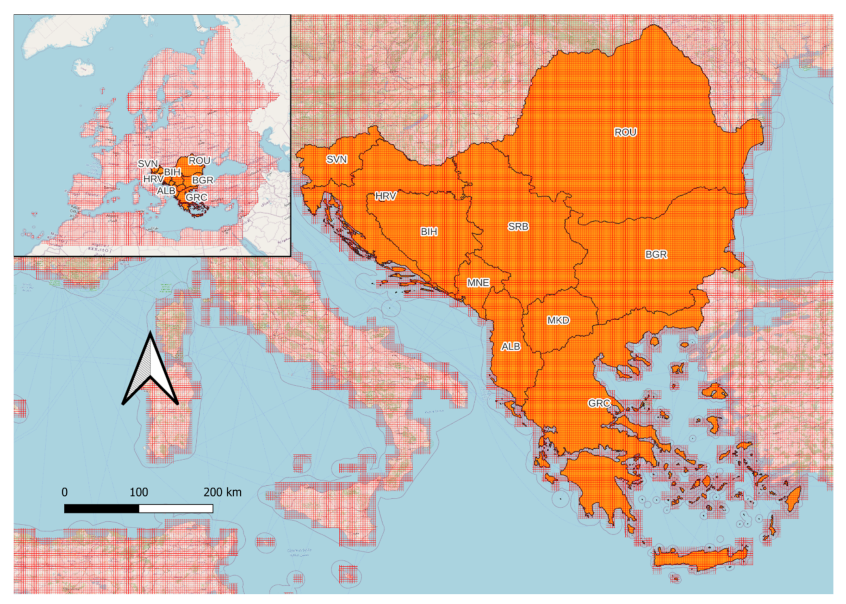
2.1. Study Area

This research focuses on the south-eastern part of the European continent, given its high potential for agricultural productivity and location in a transitional zone in terms of climatic change. The considered ten territories (Figure 1) involve Albania (ALB), Bosnia and Herzegovina (BIH), Bulgaria (BGR), Croatia (HRV), Greece (GRC), Montenegro (MNE), North Macedonia (MKD), Romania (ROU), Serbia (SRB) and Slovenia (SVN).

2.2. Data and Models

To examine the frost conditions of the study area, we utilised the fine-scale gridded dataset containing future weather data suitable for crop modelling. In the present work, the future weather dataset has been provided by simulations performed by different dynamically downscaled GCMs, accessible from the European ENSEMBLES project according to the IPCC A1B emission scenario. Nevertheless, this scenario belongs to one of the first scenarios’ family (SRES) [87], is still interesting and remains a substantial dataset in agroclimatic research [88,89].
The A1B (Figure 2) scenario represents a balanced emissions projection. Comparing the SRES family with the most widely known RCP (Representative Concentration Pathway), we could infer that in terms of overall forcing, RCP8.5 is broadly comparable to the SRES A1FI scenario, RCP6.0 to A1B and RCP4.5 to B1 [1,90]. This data was bias-corrected from three dynamically downscaled and bias-corrected regional climate simulations. Furthermore, the scenario mentioned above has been used in simulation studies extensively, representing one of the possible high-impact scenarios deriving from GHG (greenhouse gas) emissions concerning later time scales [91].
In further detail, three widely used coupled GCM-RCMs (Global Climate Model- Regional Climate Model) were employed. The first model (hereinafter denoted as DMI) consists of the ECHAM5 GCM coupled with the HIRHAM5 RCM and is run by the Danish Meteorological Institute [92]. The second model (denoted as ETH) nests CLM [93] in the HadCM3 GCM and is run by the Swiss Federal Institute of Technology.
Similarly, the third model (denoted HC) uses the same HadCM3 GCM but is coupled with the HadRM3Q0 RCM [94] and is run by the UK Met Office Hadley Centre for Climate Prediction and Research. Within the above (bias-corrected) ENSEMBLES project’s A1B realisations [95], the first and third models’ simulations are, in terms of surface air temperature, the coldest and the warmest, respectively.
Thus, the provision of an intermediate realisation with distinct precipitation patterns is accomplished by adding the second simulation model. The climate change periods of the dataset are based on three time horizons, namely 2000, 2020 and 2030. The time period covered by each horizon is 1985 to 2015 for the horizon of 2000, and it will be the reference period (henceforth RP), 2005 to 2035 for horizon 2020 (henceforth H2020) and 2015 to 2045 for horizon 2030 (henceforth, H2020). Thus, each of the above time periods covers 30 years on a daily basis. Analytic information about the dataset can be found in the meticulous paper published by Duveiller et al. [89].
The climate change dataset is available by the Agri4Cast data portal of the European Commission Joint Research Centre (https://agri4cast.jrc.ec.europa.eu/DataPortal/Indicator.aspx accessed on 2 July 2022) of the JRC MARS Meteorological Database. This one contains the daily atmospheric data to a regular 25 × 25 km grid covering a wide area from northern Africa and Near East to the Canary Islands, Scandinavian peninsula and northern (Figure 2). The emissions scenario A1B is a so-called “balanced emissions scenario” and is widely used by academia for agroclimatic and bioclimatic research [50,59,60,63,77,97].
The initial data is from synoptic weather stations, mainly in the European continent, and after an interpolation process, a freely available dataset is produced. The primary purpose of the Agri4Cast dataset is the deriving of agrometeorological indicators and crop modelling, while at the same time, it can be a valuable dataset for agroclimatic assessment [43,44]. Moreover, the Agri4Cast, according to its evaluation, has a high spatial and temporal accuracy, and this can be a reasonable basis for agroclimatic and agrometeorological research [4,45]. For the selected study area, there are 1532 grid points (Figure 2) covering canonically every part of the Balkan peninsula.
The primary reasons we choose the Agri4Cast dataset (reanalysis and climate change data) are that it is a reliable dataset with adequate accuracy, sometimes comparable to more recent datasets, such as ERAInterim and E-OBS [98], it is designed to feed the crop modelling [91,99]. The widely used .csv gridded format makes the specific dataset easy to explore, handle and use. The spatial resolution of 25 km is very suitable for such a study area because it is detailed enough but lightweight in terms of volume (gigabytes). Moreover, the temporal resolution (daily) of the dataset is optimal. The Agri4Cast dataset remains a valuable and reliable dataset for related studies [99,100,101].

2.3. Methods

Due to the large dataset and the challenging data management and analysis processes, the R-Language, which is suitable for research of this magnitude [20,86], was utilised. More specifically, R v.4.1.2 [102] core scripts and essential packages, such as the “dplyr” [103] for data handling and manipulation, “purrr” [104] and “broom” [105] for the iterating process, along with the “fst” [106], which is very fast for the reading and writing of large data frames, were employed. Initially, we handled and managed more than 46 million rows of tabular raw data.
Additionally, part of the spatial analysis and the mapping procedures were performed with the packages “raster” [107], “terra” [108] and “rgdal” [109], along with the open-source GIS software, QGIS v3.22.7 [110]. The data handling and analysis process became fully automated via the scripts, except for the map drawing. Thus, the method is partially reproducible.

2.3.1. Frost Indicators’ Calculations

The Frost Days (FD) indicator has been calculated, defined as the sum of the days where the minimum air temperature is equal to or below 0 °C [20,79]. As Biazar and Ferdosi [83] mentioned, the number of frost days can influence ecosystems, nature and human activities. The Last Spring Frost (LSF) indicator is regarded as the last frost from the beginning of the year (1 January) to 15 July, and it is a metric for the late spring’s frost.
This represents vital information because such frost events occurring after germination and budburst of herbaceous and woody plants, respectively—have an important ecological and economic impact on agriculture and forestry in temperate and boreal regions of the world [20,59,79,111,112,113]. The LSF indicator is of utmost importance, given that the plants are exceptionally susceptible to frost damage during the spring. The late spring frosts are the most dangerous in the investigated geographic area [114,115,116].
The damage induced by the late spring frosts to vulnerable plant organs markedly affects plants’ growth, vigor, competitive ability and distribution limits, causing more economic losses to agriculture than any other climate-related hazards [117]. Moreover, the Free of Frost Days (FFD) indicator expresses the free of frost period of the year, which is calculated indirectly as the period between estimated indicators designated as the Last Spring Frost (LSF) and the First Autumn Frost (FAF). The FAF is defined as the first frost day (Julian day) after 15 July to the end of the year.
The spatial distributions of the indicators have been made by interpolating the gridded data values. Specifically, the ordinary kriging method was implanted, taking advantage of the regularly placed gridded data [118,119].

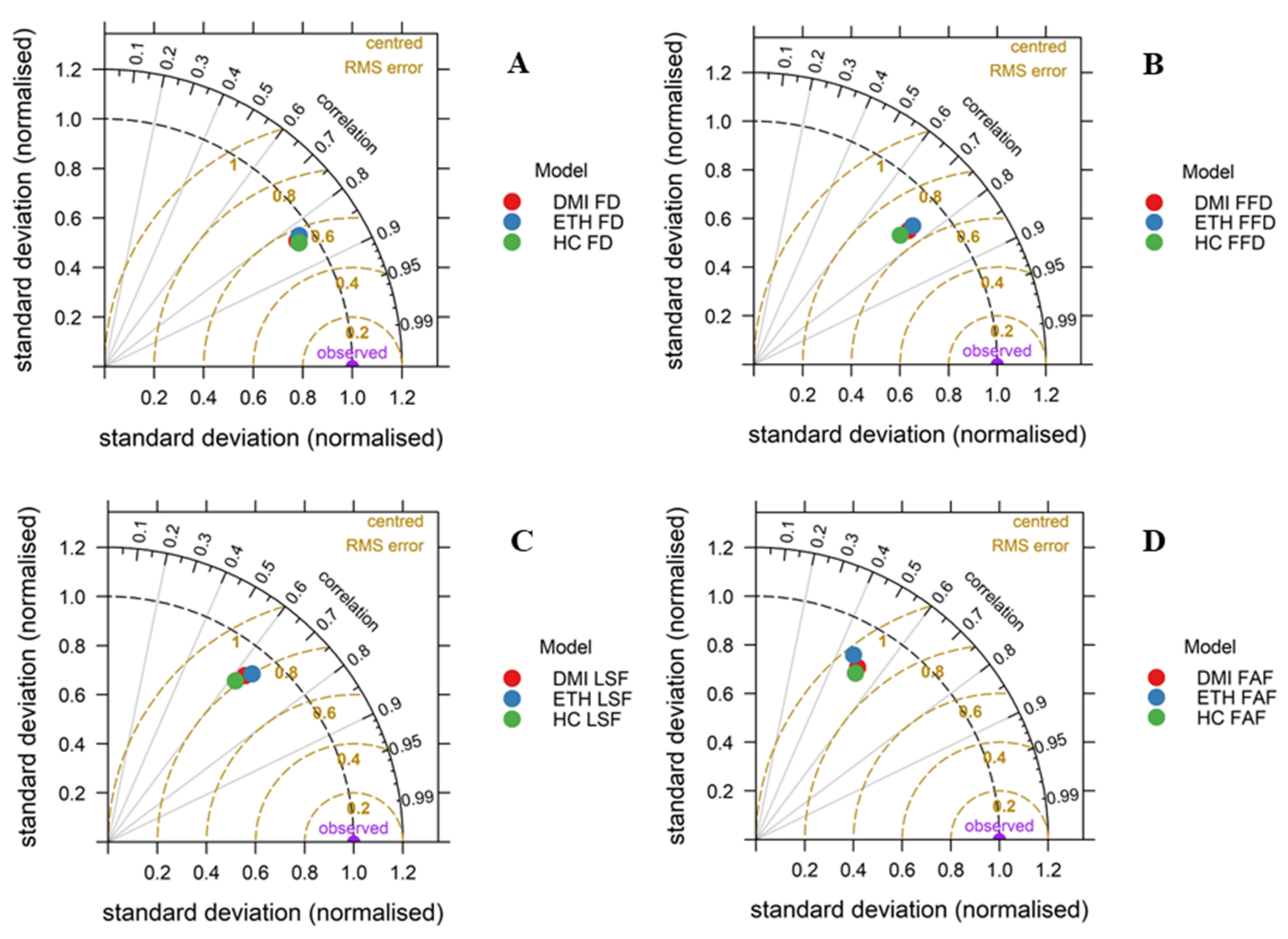
2.3.2. Models’ Comparison

In order to select the most accurate model for the analysis of future frost indicators, we conducted a comparison between the frost indicators (FD, FFD, LSF and FAF), which have been calculated by the observed data (of the Agri4Cast) and the frost indicators of the climatic models. The common period for the observed atmospheric parameters and the estimations of the climate change models is from the year 1985 to the year 2014. For the above period, the frost indicators were calculated by the observations’ of the Agri4Cast dataset and for the same grid points, calculated the indicators by the models of DMI (DMIHIRHAM5-ECHAM5), ETH (ETHZ-C
LMHadCM3Q0) and HC (METO574-HC-HadRM3Q0-HadCM3Q0). The Taylor diagram (Figure 3) was used to evaluate the accuracy of the climate models, given that it can combine three statistical metrics in a 2D graph [56,120,121]. The diagrams have been drawn using the “openair” R-package [122] along with “dplyr” [103] and “reshape2” [123] packages.
The performance of the models is almost identical for the four frost indicators. Overall, we can assume that HC is the best model because it scores the lowest standard deviation for FFD and LSF, has the highest correlation for the FD and FAF and has the lowest RMS error for FAF and FD.

3. Results

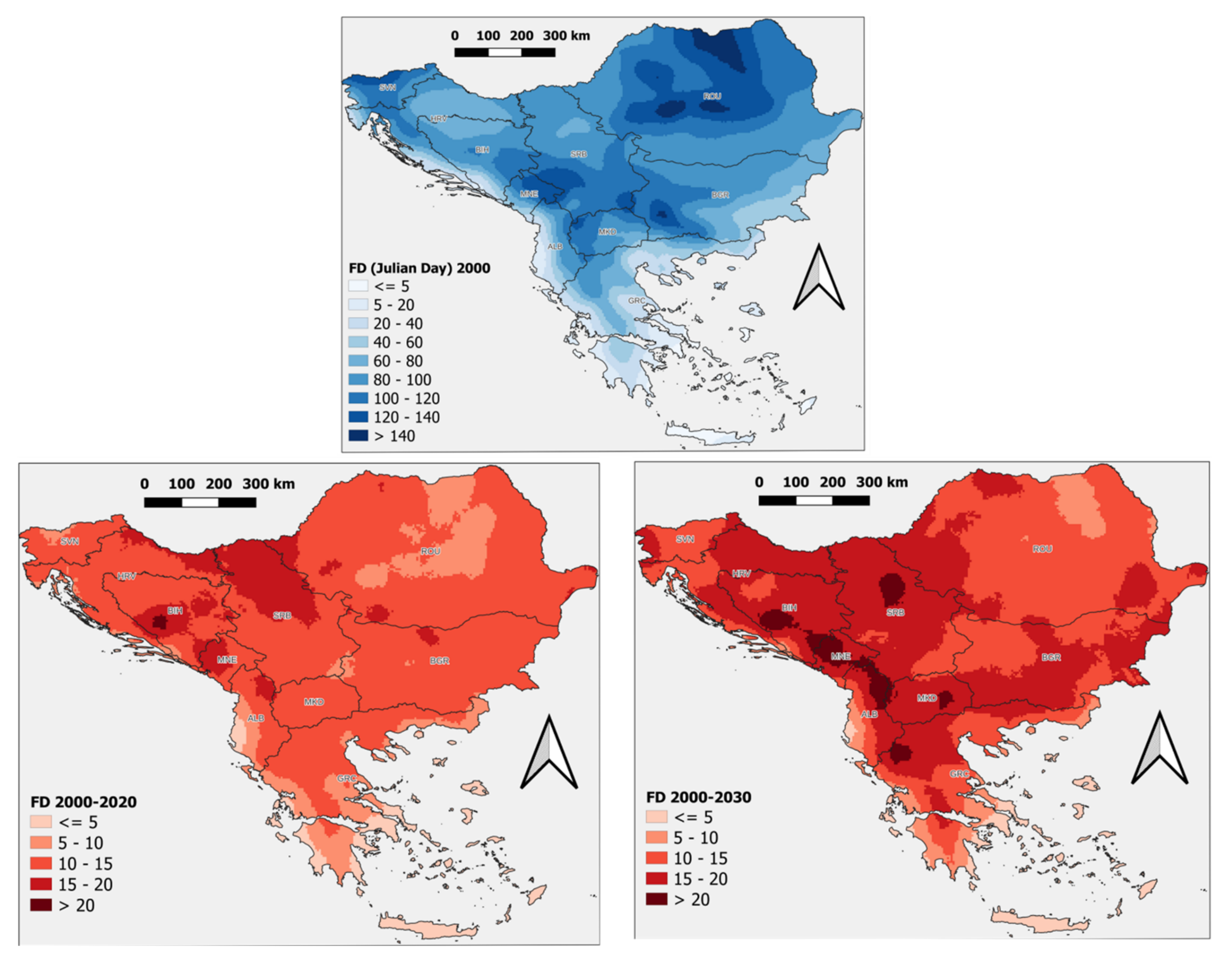
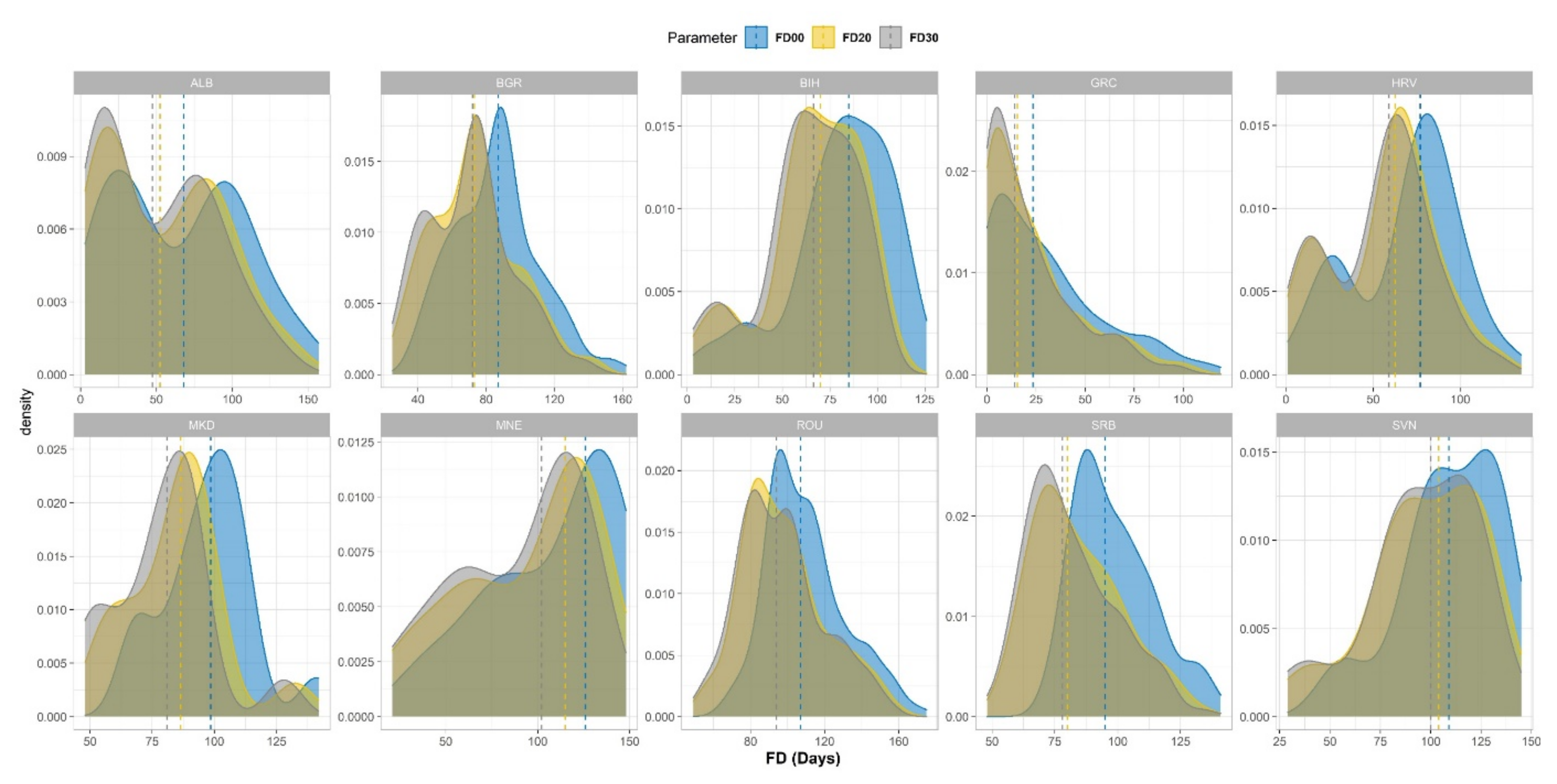
3.1. Frost Days (FD)

The most frequently used frost indicator is the total amount of frost days (FD) on a yearly basis (Figure 4). In the study area, the FDs spatial distribution of the RP is affected by both the latitude and altitude. Thus, high values (>140) of FDs are calculated over the northern Carpathians and a very low number of FDs (<20) over the coastal areas of the Aegean and Adriatic seas. As anticipated, the lowlands on either side of the Romano-Bulgarian borders show relatively low FDs values (40–80). Low values of FDs are also recorded over the borders of Croatia (HRV) and Bosnia Herzegovina (BIH). Over the mountainous region of eastern Montenegro (MNE), the FD values are relatively high (>100).
At the left-down map of Figure 4, where the difference between the RP and the H2020 is depicted, only positive values indicating a reduction of FDs, due to climate change are observed. The highest reduction is recorded over central Bosnia and Herzegovina, with values >20 days per year. High values of reduction are recorded over northern Serbia. It is worth noting that the lowest reduction is anticipated over the areas with low FD values, such as southern Greece and western Albania.
The density plots (Figure 5) reveal the distribution of the FD values over each country and their evolution due to the climate change projections. The vertical-coloured dashed lines represent the median; their values can be found in Table 1. It is evident that the FD value is decreasing from the reference period to the H2020 and H2030, respectively. The higher reduction in the FDs values from the reference period to the H2020 is recorded over Greece. The median of the reference period is 23.5 FDs and at the H2020 is 15.5 FDs (a reduction of 34%), while the reduction from the reference to the H2030 is 40.4 FDs.
A high reduction is recorded over Albania, from a median of 68 FDs at the reference period to 52.5 in 2020 and 47.5 in the H2030, indicating a reduction of 22.8% and 30.1% (Table 2), respectively. The kernel density plot of Albania (ALB) indicates a bimodal variation of FD over the country, revealing the frost days’ regime contrast between mountainous and coastal Albania.
The lowest reduction of FDs is recorded in Slovenia, as seen in the density plots graph (Figure 5) and the medians’ statistics (Table 1 and Table 2). In general, the lower reduction of frost days is projected over the areas with a relatively low number of FDs, such as southern Greece and coastal Albania. In comparison, a higher reduction is anticipated in the regions with high FDs, such as the mountainous areas of Montenegro and Serbia, northwestern Greece and central Bosnia and Herzegovina. Thus, the FDs evolution would lead to biophysical alterations of the natural south-eastern European areas.
Similarly to the presented research, Ruml et al. [61] found that fewer frost days (FD) are projected over the Serbian territory. In more detail, a reduction in frost frequency of around 10 days is expected in the following decades and a reduction of 45 days at the end of the century. Finally, the authors concluded that there would be no risk of winter damage to grapevines due to extreme cold in the Serbian territory by the end of the century. For the same time frame, Mihailović et al. [62] found that the FD in Serbia will decrease by approximately five times.
In corroboration with the above results, Georgoulias et al. [124] found that the FDs are projected to decrease over Greece for more than 10 days in the near future according to the RCP4.5 and RCP8.5 emissions scenarios. They calculated that the FD would be reduced by 28 days at the end of the century, according to RCP8.5. Moreover, the FDs spatial distribution is mainly identical to the findings of this study.
Recently published studies about climate change in the Western Balkans region [5,17] found similar results, regarding the quantity and the spatiotemporal distribution of FD and their evolution due to climate change, for Albania, Croatia, Serbia, North Macedonia and Montenegro found. More specifically, the authors found a potential decrease of 10–20 FDs according to the RCP4.5 emissions scenario, comparing their reference period 1986–2005 with the 2046–2065 period and an even higher reduction according to the RCP8.5 scenario.
Detailed research by Burić and Doderović [114] examined the climatic projection of cardinal atmospheric parameters and indicators over Montenegro and found results that are in general agreement with the present research, indicating a future decrease of FD over the examined territory. In general, the future reduction of FD is expected as a consequence of global and regional warming due to climate change [27,99].

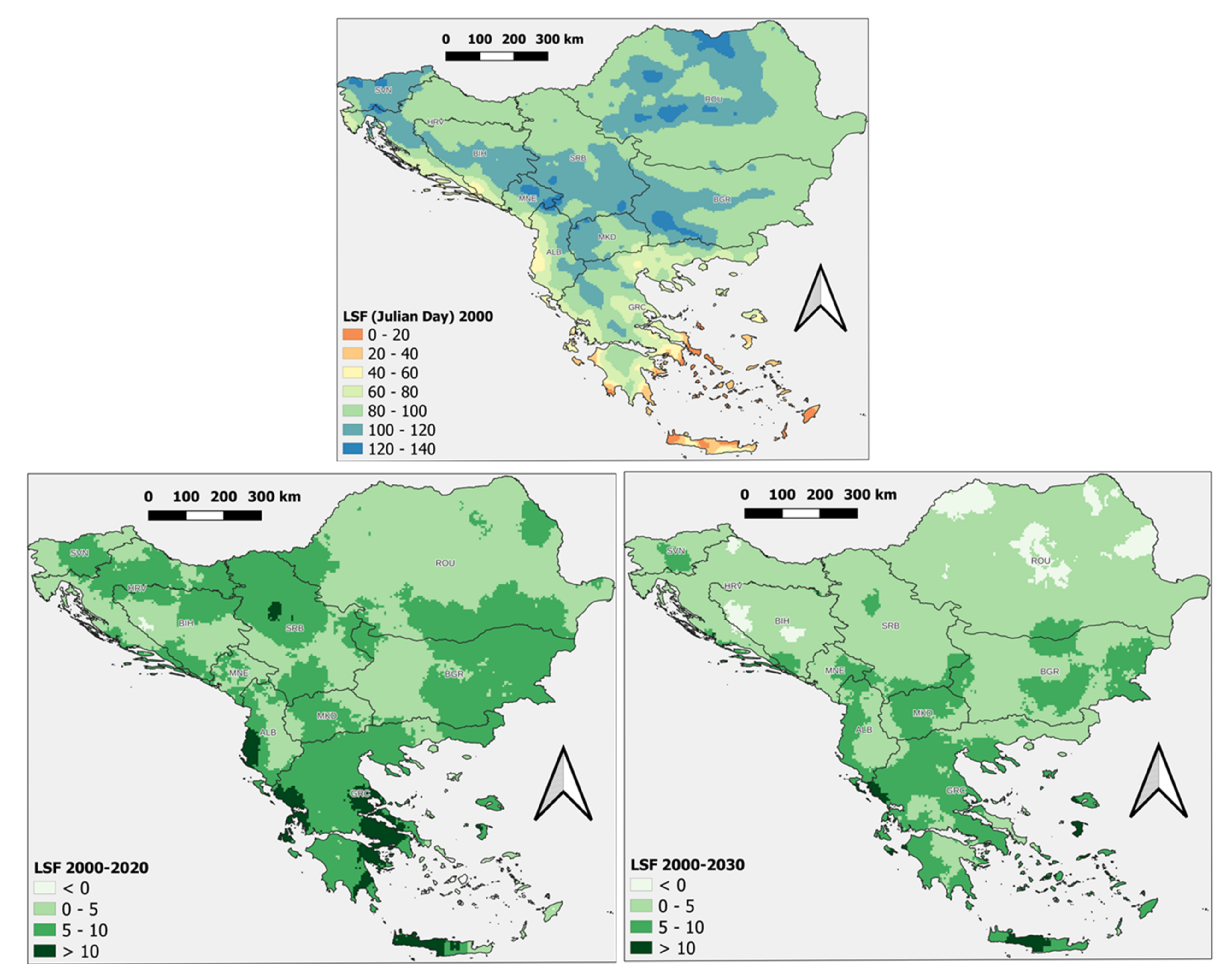
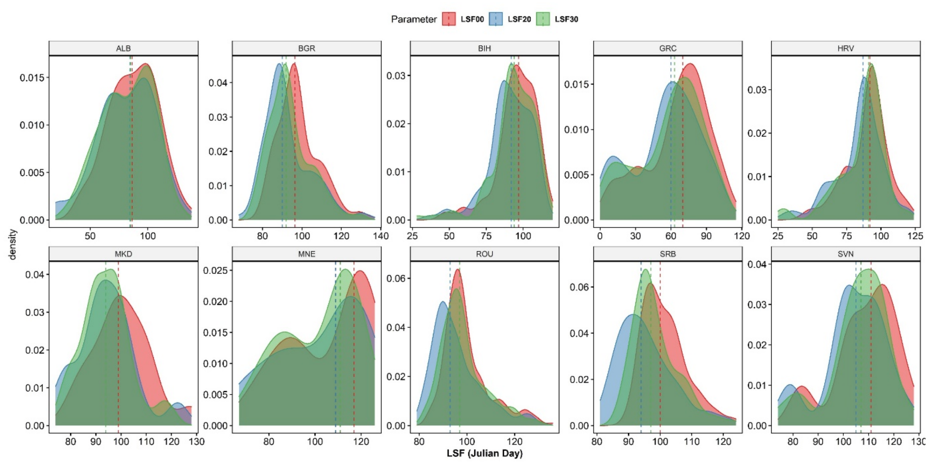
3.2. Last Spring Frost (LSF)

The Julian day of the LSF determines the start of the growing season. As already mentioned, LSF is an important indicator for the assessment of the climatic suitability of the region in terms of agriculture. The following graph (Figure 6) shows the spatial distribution of the LSF Julian day over the study area for the RP in the upper image and the differences between the LSF’s distribution of the H2020 (right) and H2030 (left) from the reference period. It is pinpointed that the higher the LSF value is, the risk of crop damage (due to frost) is more possible, and at the same time, the growing season is becoming narrower.
We observed that, over southern Greece and the Aegean Sea, the LSF frequently occurs before the 20th day of the year, which is practically interpreted as the absence of the spring frost. Similarly to the above, low LSF values are recorded over the Adriatic coast of Albania and Croatia, indicating an almost free of frost spring period. On the other hand, the high LSF values mean delayed spring frost over the Carpathians in central and northern Romania, over the Rhodope mountains (the southern part of Bulgaria near the Greek borders and the mountainous region of Montenegro).
The LSF value of 120–140 means that a frost occurs during the first 20 days of May when the crops may be fully active regarding plants’ biology. The most frequent classes of LSF over the agricultural areas are 60–80 and 80–100, which are clarified as the frost occurrence on the first 20 days of March, the last ten days of March and the first ten days of April, respectively.
As shown in Figure 6, the advancement of LSF is anticipated for H2020 due to climate change. That is why the spatial distribution of the LSF differences draws only positive values. This means that the potential risk of spring frost damage in the study area may be lower by H2020. The higher advancement has been recorded over central Greece and the western part of Crete Island, counting values higher than 10 Julian days. Moreover, the high advancement of LSF in central Serbia is evident.
It is highlighted that the differences between the H2030 and reference period are lower than the related H2020. Thus, the potential risk will be higher during H2030 compared to H2020.
In Figure 7, the evolution of the Julian days distributions for the three studied time horizons and the corresponding medians are depicted, while in Table 1, their respective values are presented. The higher temporal change is recorded over Greece with a decrease from 70 Julian days during the reference period to 60 during H2020 (a decrease of 14.3%). During H2030, the decrease is lower, counting 63 Julian days (a decrease of 10%). On the contrary, the lowest decrease in the LSF median is recorded over Albania, from 86.5 during the reference period to 84.5 Julian days during the H2020 (a decrease of 2.3%). The decrease over Albania is more limited during the H2030 with a median of 85 Julian days.
It is evident that most kernel density distributions are unimodal (with one major pick) except for Montenegro (MNE), Slovenia (SVN) and Greece (GRC). The bimodal distribution is formed owing to the country’s geography, which forms two (almost) distinct LSF regimes, one caused by the high-altitude areas and the other caused by the lowlands or the warmest areas.
In corroboration with the above findings, Ruml et al. [61] indicated that Serbia’s viticultural areas will experience earlier frost (LSF). Moreover, a previous study [17] demonstrated that the LSF trends revealed the highest delays (higher Julian days) over coastal Albania.

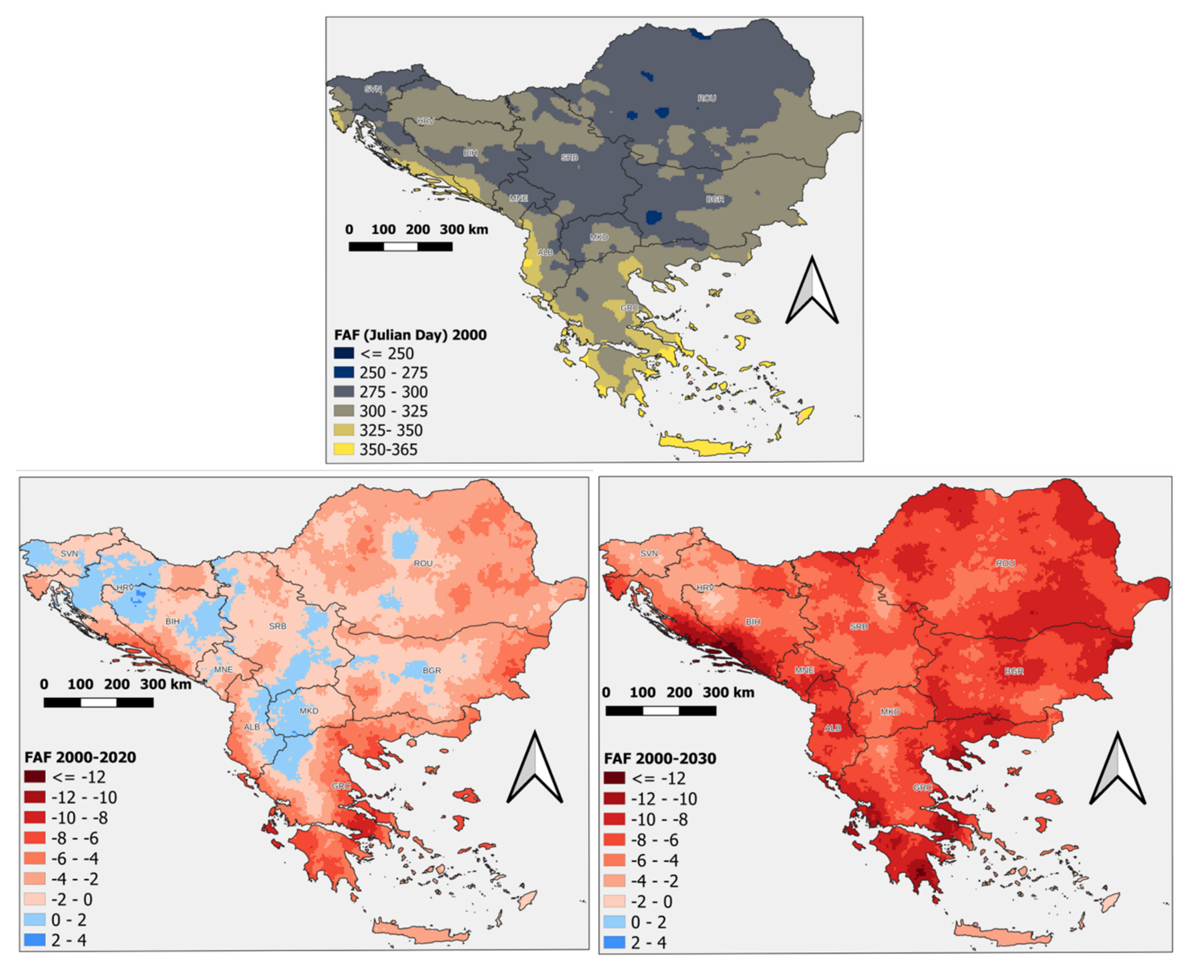
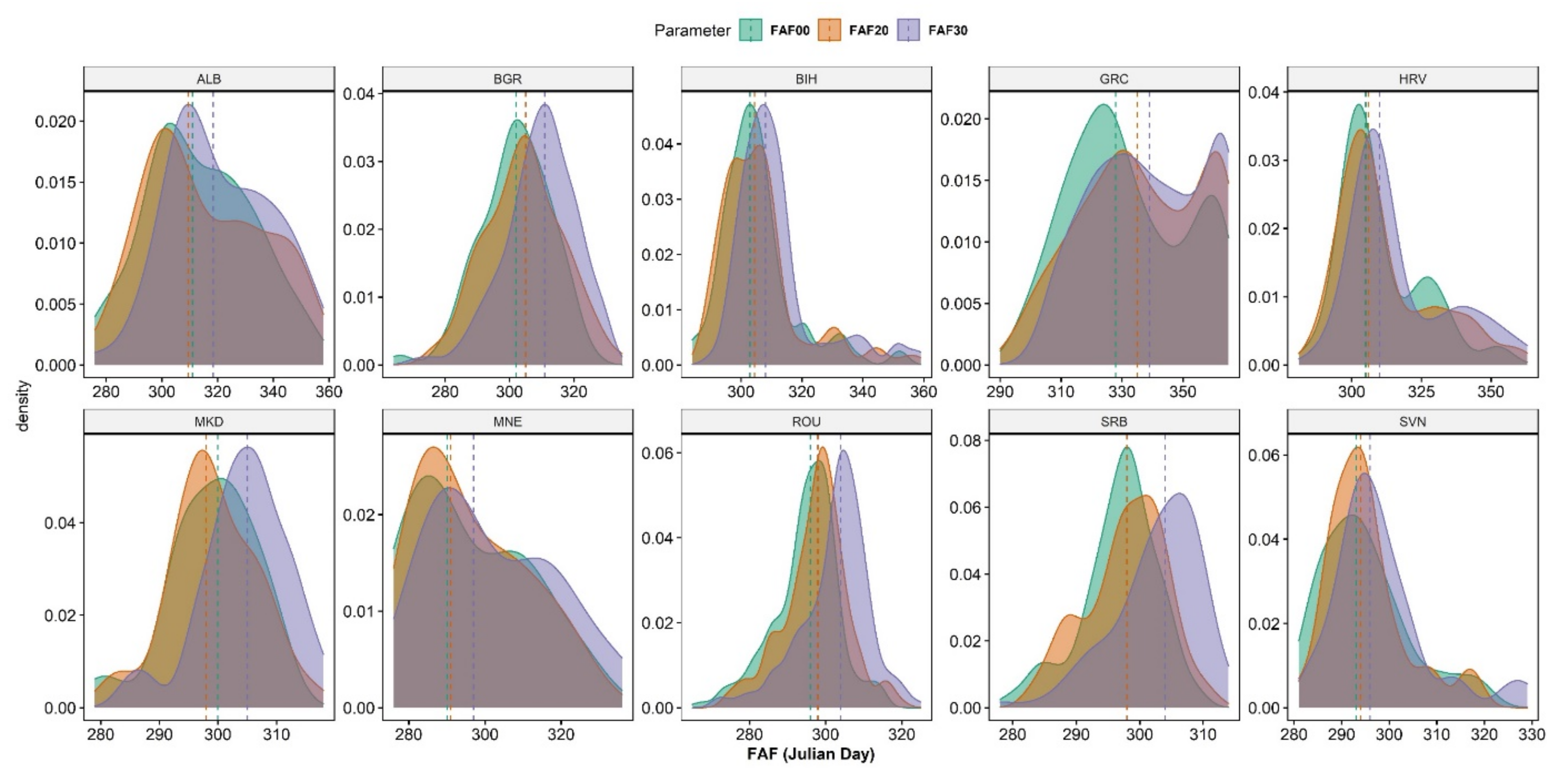
3.3. First Autumn Frost (FAF)

The First Autumn Frost (FAF) indicates the end of the growing season in a specific area and the beginning of the low temperatures. Figure 8 shows the spatial distribution of FAF in Julian days during the RP in the upper central image, along with the difference between the reference period and the H2020 (down right) and the difference between the reference period and the H2030 (down left), respectively.
The highest FAF values occur over coastal Greece and over the Adriatic seashore (particularly in Albania and Croatia), indicating a relationship between the altitude and the FAF values. Over these areas, the first frost following the summer period is anticipated after the mid of December. Over the adjacent areas with higher altitudes the first frost (FAF) occurs after the 21 November. The third category of the FAF spatial distribution, which covers most of the study area, represents the time period from 27 October to 20 November.
This category covers the half-eastern part of Bulgaria, the mountainous part of Greece and Albania, the southern part of North Macedonia and the plain areas of Serbia, Croatia and Bosnia and Herzegovina. The next earlier category (275–300 Julian days) represents the period between 2 October and 27 October covering the higher areas in terms of altitude, in which the agricultural activity is more sparce. Thus, during the reference period, the first autumn frost is not so close to the summer period (when the plants are more biologically active).
The image depicting the difference between the H2000 and the H2020 (Figure 8, left down) reveals that most of the study area is under negative values. This means that the FAF value is becoming higher from the H2000 to the H2020. Thus, the evolution of the areas under this regime indicates an extension of the growing season due to climate change. The areas expected to be subjected to this characteristic evolution involve the coastal countries, particularly Greece and the Adriatic shoreline of Albania and Croatia, along with the lowland of the examined countries.
On the contrary, over the areas with higher altitudes, a positive difference between H2000 and H2020 has been calculated, indicating a reduction of the FAF values. This means that over these areas, the potential growing season will become shorter. On the other hand, the image with the difference between RP and H2030 indicates an increase over all the studied areas. The phenomenon of the delayed autumn frost is more evident in southern Peloponnese, in western Greece and over the Adriatic coastal areas of Croatia and Bosnia and Herzegovina. High negative values have been recorded over the southern Romanian plain area.
In Figure 9, the density plots of the FAF per time horizon and per country are displayed, and in Table 1, the medians of these distributions are listed. It is worth noting that in most countries, the median is becoming lower from the RP to the H2020; after that, to the H2030, there is a slight increase. Specifically, in the case of Romania, the FAF median is 97 for the reference period, becomes equal to 93 for the H2020 and then returns to 97 Julian days for the H2030.
According to Table 1 and Table 2, only Albania and North Macedonia demonstrate positive median values, as shown by the difference in the reference period and the H2020, which means that in the near future, the FAF is expected to occur earlier. On the contrary, the highest negative values have been recorded for Greece (−2.1%) and Bulgaria (−1.0%). The related differences between the reference period and the H2030 reveal negative values for all the studied countries, with higher values of −3.4%, −3%, −2.7% for Greece, Bulgaria and Romania, respectively). The FAF distributions’ general image reveals that south-eastern Europe will experience delayed FAF due to climate change, thus facing reduced related risk and enlengthening the growing season.
The above results align well with the findings of the previously published research by Ruml et al. [59], which concluded that in the Serbian viticultural areas, the (FAF is expected to occur a few days later, even in mountainous areas. Similar results in terms of the FAFs spatial distributions over the same area have been found by Charalampopoulos [17], in which the trends of the FAFs increase in the near future are demonstrated.

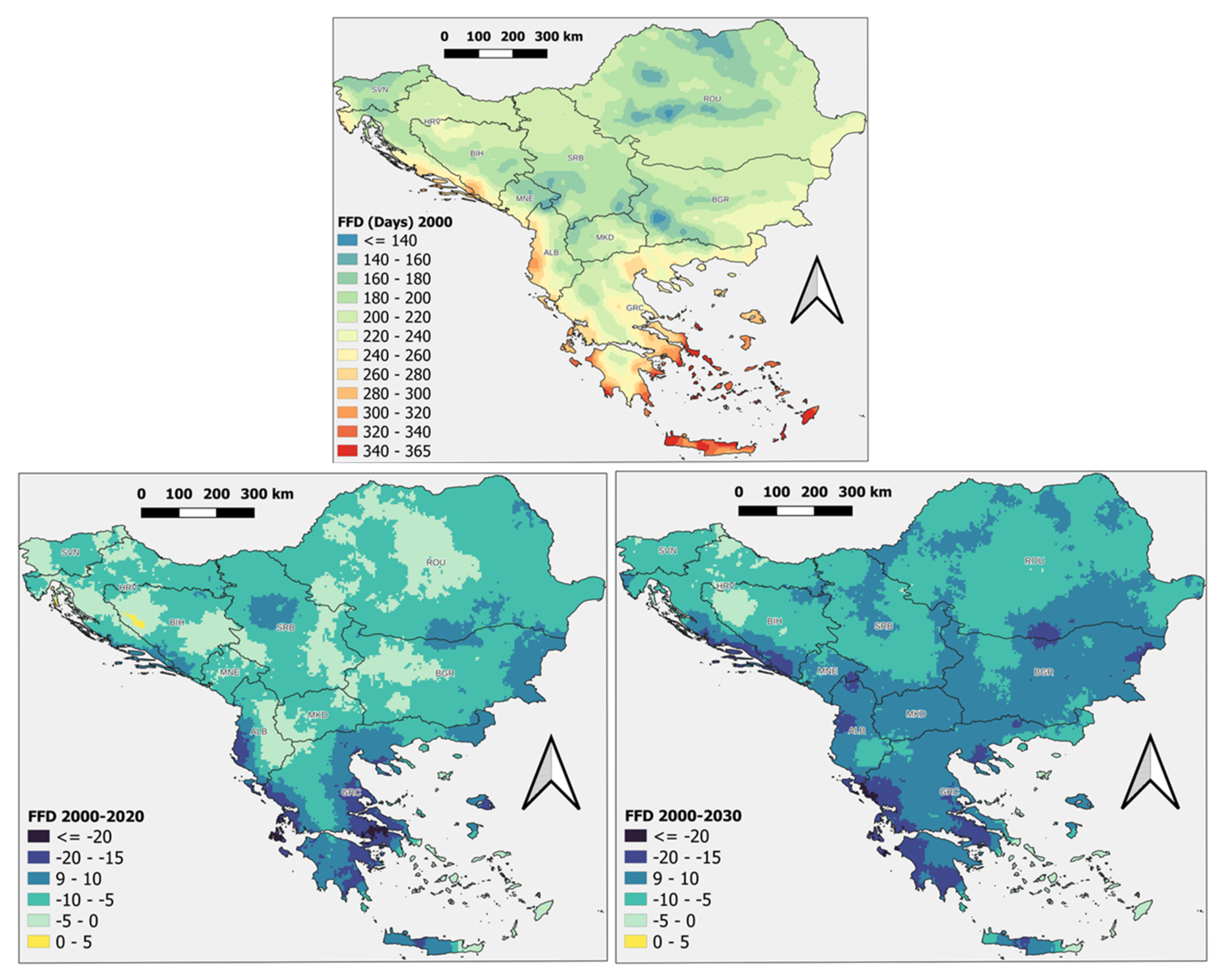
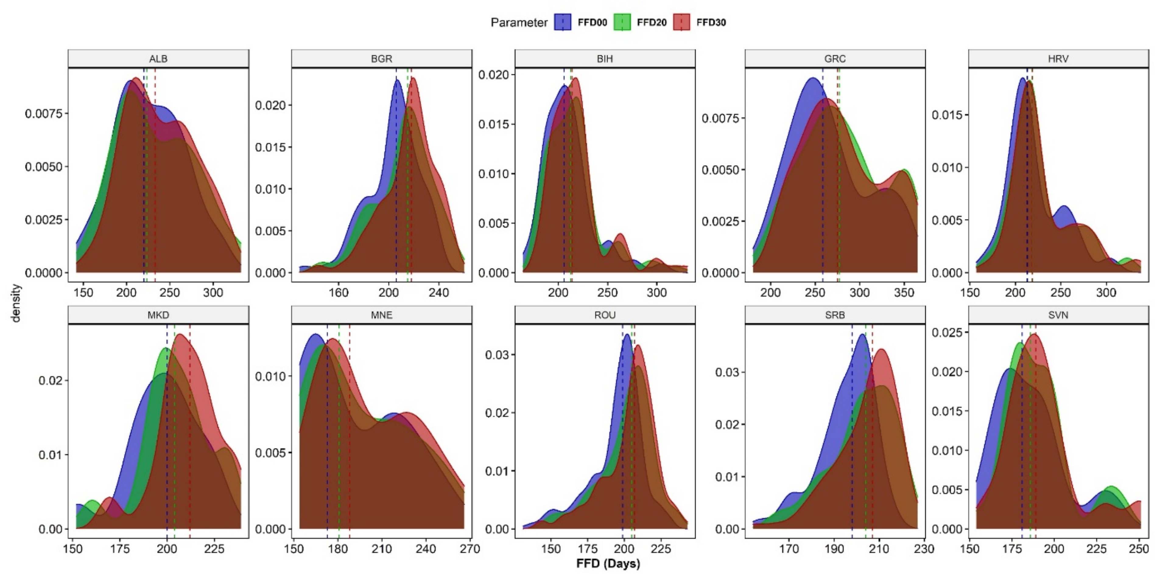
3.4. Free of Frost Days (FFD)

The Free of Frost Days (FFD) indicates a time span of an uninterrupted growing season from the frost phenomenon and is calculated as the number of consecutive days without frost.
The following, Figure 10 is depicted the spatial distribution of FFD values for the RP in the upper image, the spatial distribution of the difference between the reference period and the H2020 in the lower left image and the spatial distribution of the difference between the reference period and the H2030 in the lower right image.
As anticipated, a higher amount of FFDs during the reference period is recorded over the south-eastern part of the study area. Especially the islands of the Aegean Sea and the southern Peloponnese are annually almost free of frost conditions. High FFD values (<270 days) are spotted in Thessaloniki’s plain (northern Greece), on the central Albanian shoreline, in the coastal area of Croatia and over Bosnia and Herzegovina. The median values displayed in Table 1 and Table 2 at the country level reveal recorded annual values of 258.5 days for Greece, 220 days for Albania and 215 days for Croatia. On the other hand, the countries with the lower FFD values are Montenegro with 173, Slovenia with 181 and Serbia with 198 days per year.
According to the down-left image (Figure 10), negative values cover almost the total of the studied area. This means that the FFD value is anticipated to be higher at the H2020 than at the RP and indicative of a lowering frost risk in the south-eastern European area due to climate change. Only the western part of Bosnia and Herzegovina recorded a spot of a low positive difference.
The higher negative values (a relative increase from the reference period to the H2020), higher than 15 days per year, have been recorded over the central and the western part of Greece. A high increase of FFDs during H2020 has also been recorded over the coastal part of Albania. Relatively high FFDs increase has been recorded over the northeastern part of the study area in the territories of Greece and of Bulgaria.
The increasing trend of the FFDs due to climate change is evident during the H2030 (down-right graph). The overview of this distribution is an enhanced increase of the FFDs over the entire study area. Thus, during the H2030, Greece counts a median of 275 days per year (6.4% increase by the reference period), North Macedonia of 212 days per year (6.0% increase) and Albania of 233 days per year (5.9% increase). The lowest increase has been recorded in Croatia (2.6%), with a median of 218.5 days per year during the H2030. Bosnia and Herzegovina display a relatively low increase of FFDs, which counts a median of 214 days per year (3.9% increase). It is also evident that the trend of the FFDs increase is lower during the H2030 than the relative trend of the H2020, likely because of the A1B emissions scenario.
Figure 11 shows the kernel density of the FFDs of each country and displays the distribution of the values and their temporal shift with the median depicted by the vertical dashed lines. It is evident that the FFDs demonstrate the same tendency over all the selected countries in the south-eastern part of Europe owing to the employed emissions scenario.
Binomial distributions result in countries with extended coastal and mountainous zones, such as Greece and Croatia and more unified distributions in countries with balanced geography, such as Romania and Serbia. It is evident that over most of the countries, the shift of the kernel density curve is wider from the RP to the H 2020 compared with the shift from the H2020 to the H2030.
The big picture of the FFDs evolution due to climate change in south-eastern Europe is that a higher increase is expected over the Adriatic Sea and Ionian Sea (Greece) coast and in southern Greece. Some spots of the FFDs’ increase result for the plain area of northern Serbia, the plain area of the Bulgaro-Romanian borders and the coastal and northern Albania. The above findings are in alignment with the results of a previous study [40] in which it is mentioned that Bosnia and Herzegovina will face a longer free of frost period (higher number of FFDs) due to climate change.
The free of frost period is expected to be enlengthened in the traditional viticultural areas of Serbia (average prolongation of 15 days by 2030 and 45 days by 2100), according to Ruml et al. [61]. The climate change projections indicate warming over the study area along with dryer conditions [27,99,100,125,126]. The findings of this study are consistent with the previous conclusions because the rising of temperature drives to an expansion of the free of frost period.

4. Concluding Remarks

The present research aimed to explore the frost projections for south-eastern Europe via a high spatial resolution dataset containing three climate models for the three-time horizons according to the A1B emissions scenario. In order to select the most accurate model, a comparative analysis was conducted, and the Taylor diagram presents its results. The HC (METO574-HC-HadRM3Q0-HadCM3Q0) model demonstrated slightly more accuracy compared with the ETH (ETHZ-CLMHadCM3Q0) and the DMI (DMIHIRHAM5-ECHAM5) models employed for the estimation of the calculated frost indicators as shown in the Taylor diagrams.
Due to climate change over south-eastern Europe, the frost days (FD) are expected to be reduced according to the balanced A1B emissions scenario. The areas with a higher number of FDs will face the highest reduction. Thus, the mountainous and the continental regions will be most affected by facing the highest FDs decrease, followed by related ecological/agricultural consequences.
The statistics and the spatial distributions of the LSFs present a clear image of reduction for both horizons. During the H2020, a higher reduction (compared to the reference period) is expected over Greece and Albania. However, during the H2030, there was a recession of the LSFs differences, likely because of the slight emissions’ reduced rate of A1B scenario.
According to the FAFs indicator, over the lowlands and the coastal areas, during the H2020 compared with the RP, the first frost after the summer will be delayed. For the same horizon (2020), the areas with high altitudes are expected to face earlier FAF. During the H2030, all the studied areas are projected to face delayed FAF without exceptions.
In general, we demonstrated that the south-eastern European territory will face an increase in the growing season duration due to the increase of the FFDs, without exceptions. This outcome is potentially beneficial for the agricultural sector but is questionable when considering the impacts on the ecological balance of the natural and conservation areas.
Managing an extensive environmental dataset, such as Agri4Cast, allows coding (in this case, with R language) to become an essential tool for analysing and visualising the results. Finally, the analysis dataset is publicly available in an open repository for the research community’s use for future studies.

Author Contributions

Conceptualisation, I.C.; methodology, I.C.; investigation, I.C. and F.D.; resources, I.C. and F.D.; data analysis and visualisation, I.C.; writing—original draft preparation, I.C. and F.D.; writing—review and editing, I.C. and F.D.; supervision, I.C. All authors have read and agreed to the published version of the manuscript.

Funding

This research received no external funding.

Institutional Review Board Statement

Not applicable.

Informed Consent Statement

Not applicable.

Data Availability Statement

The results data presented in this study are openly available in Zenodo at https://doi.org/10.5281/zenodo.6961647 (accessed on 5 August 2022).

Conflicts of Interest

The authors declare no conflict of interest.

References

  1. Pachauri, R.K.; Allen, M.R.; Barros, V.R.; Broome, J.; Cramer, W.; Christ, R.; Church, J.A.; Clarke, L.; Dahe, Q.; Dasgupta, P. Climate Change 2014: Synthesis Report. Contribution of Working Groups I, II and III to the Fifth Assessment Report of the Intergovernmental Panel on Climate Change; IPCC: Geneva, Switzerland, 2014; ISBN 92-9169-143-7. [Google Scholar]
  2. Leal Filho, W.; Trbic, G.; Filipovic, D. Climate Change Adaptation in Eastern Europe: Managing Risks and Building Resilience to Climate Change; Springer: Berlin/Heidelberg, Germany, 2018; ISBN 3-030-03383-X. [Google Scholar]
  3. Nastos, P.T.; Zerefos, C.S. Spatial and Temporal Variability of Consecutive Dry and Wet Days in Greece. Atmos. Res. 2009, 94, 616–628. [Google Scholar] [CrossRef]
  4. Bindi, M.; Olesen, J.E. The Responses of Agriculture in Europe to Climate Change. Reg. Environ. Chang. 2011, 11, 151–158. [Google Scholar] [CrossRef]
  5. Knez, S.; Štrbac, S.; Podbregar, I. Climate Change in the Western Balkans and EU Green Deal: Status, Mitigation and Challenges. Energy Sustain. Soc. 2022, 12, 1. [Google Scholar] [CrossRef]
  6. Županić, F.Ž.; Radić, D.; Podbregar, I. Climate Change and Agriculture Management: Western Balkan Region Analysis. Energy Sustain. Soc. 2021, 11, 51. [Google Scholar] [CrossRef]
  7. Lelieveld, J.; Hadjinicolaou, P.; Kostopoulou, E.; Chenoweth, J.; El Maayar, M.; Giannakopoulos, C.; Hannides, C.; Lange, M.A.; Tanarhte, M.; Tyrlis, E.; et al. Climate Change and Impacts in the Eastern Mediterranean and the Middle East. Clim. Chang. 2012, 114, 667–687. [Google Scholar] [CrossRef] [PubMed]
  8. Gaál, L.; Beranová, R.; Hlavčová, K.; Kyselý, J. Climate Change Scenarios of Precipitation Extremes in the Carpathian Region Based on an Ensemble of Regional Climate Models. Adv. Meteorol. 2014, 2014, e943487. [Google Scholar] [CrossRef]
  9. Oikonomou, C.; Flocas, H.A.; Hatzaki, M.; Asimakopoulos, D.N.; Giannakopoulos, C. Future Changes in the Occurrence of Extreme Precipitation Events in Eastern Mediterranean. Glob. NEST J. 2008, 10, 255–262. [Google Scholar]
  10. Olesen, J.E.; Bindi, M. Consequences of Climate Change for European Agricultural Productivity, Land Use and Policy. Eur. J. Agron. 2002, 16, 239–262. [Google Scholar] [CrossRef]
  11. Trajkovic, S.; Milanovic, M.; Milicevic, D.; Gocic, M. The Assessment of Exposure to Climate Change in South-Eastern Serbia Regions. Int. Multidiscip. Sci. GeoConference SGEM 2020, 20, 491–498. [Google Scholar]
  12. Droulia, F.; Charalampopoulos, I. A Review on the Observed Climate Change in Europe and Its Impacts on Viticulture. Atmosphere 2022, 13, 837. [Google Scholar] [CrossRef]
  13. European Environment Agency Climate Change. Impacts and Vulnerability in Europe 2016: An Indicator-Based Report; Publications Office: Luxembourg, 2017. [Google Scholar]
  14. Custovic, H.; Ðikic, M.; Ljusa, M.; Zurovec, O. Effect of Climate Changes on Agriculture of the Western Balkan Countries and Adaptation Policies. Poljopr. Sumar. 2012, 58, 127. [Google Scholar]
  15. Unkašević, M.; Tošić, I. Trends in Temperature Indices over Serbia: Relationships to Large-Scale Circulation Patterns. Int. J. Climatol. 2013, 33, 3152–3161. [Google Scholar] [CrossRef]
  16. Burić, D.; Luković, J.; Ducić, V.; Dragojlović, J.; Doderović, M. Recent Trends in Daily Temperature Extremes over Southern Montenegro (1951–2010). Nat. Hazards Earth Syst. Sci. 2014, 14, 67–72. [Google Scholar] [CrossRef] [Green Version]
  17. Vuković, A.; Vujadinović Mandić, M. Study on Climate Change in the Western Balkans Region; Bosnia and Herzegovina; Regional Cooperation Council Secretariat: Sarajevo, Bosnia and Herzegovina, 2018. [Google Scholar]
  18. Bucur, G.M.; Dejeu, L. Researches on Situation and Trends in Climate Change in South Part of Romania and Their Effects on Grapevine. Sci. Pap. Ser. B Hortic. 2017, 61, 243–247. [Google Scholar]
  19. Kostopoulou, E.; Jones, P.D. Assessment of Climate Extremes in the Eastern Mediterranean. Meteorol. Atmos. Phys. 2005, 89, 69–85. [Google Scholar] [CrossRef]
  20. Charalampopoulos, I. Agrometeorological Conditions and Agroclimatic Trends for the Maise and Wheat Crops in the Balkan Region. Atmosphere 2021, 12, 671. [Google Scholar] [CrossRef]
  21. Doderović, M.; Burić, D.; Ducić, V.; Mijanović, I. Recent and Future Air Temperature and Precipitation Changes in the Mountainous North of Montenegro. J. Geogr. Inst. Jovan Cvijic SASA 2020, 70, 189–201. [Google Scholar] [CrossRef]
  22. Popov, T.; Gnjato, S.; Trbić, G. Changes in Temperature Extremes in Bosnia and Herzegovina: A Fixed Thresholds-Based Index Analysis. J. Geogr. Inst. Jovan Cvijic SASA 2018, 68, 17–33. [Google Scholar] [CrossRef]
  23. Bonacci, O. Air Temperature and Precipitation Analyses on a Small Mediterranean Island: The Case of the Remote Island of Lastovo (Adriatic Sea, Croatia). Acta Hydrotech. 2019, 32, 135–150. [Google Scholar] [CrossRef]
  24. Doko, A.; Krasniqi, S.; Fyshku, A.; Topi, I.; Kopali, A. Analysis of Climatic Variability and Determination of Thermal and Pluviometric Limits in Albania’s Southwestern Lowland Area (Vlora). Mech. Agric. Conserv. Resour. 2020, 66, 184–189. [Google Scholar]
  25. Dumitrescu, A.; Bojariu, R.; Birsan, M.-V.; Marin, L.; Manea, A. Recent Climatic Changes in Romania from Observational Data (1961–2013). Theor. Appl. Climatol. 2015, 122, 111–119. [Google Scholar] [CrossRef]
  26. Ionita, M.; Chelcea, S.; Rimbu, N.; Adler, M.-J. Spatial and Temporal Variability of Winter Streamflow over Romania and Its Relationship to Large-Scale Atmospheric Circulation. J. Hydrol. 2014, 519, 1339–1349. [Google Scholar] [CrossRef]
  27. Pörtner, H.-O.; Roberts, D.C.; Adams, H.; Adler, C.; Aldunce, P.; Ali, E.; Begum, R.A.; Betts, R.; Kerr, R.B.; Biesbroek, R. Climate Change 2022: Impacts, Adaptation and Vulnerability; Cambridge University Press: Cambridge, UK; New York, NY, USA, 2022. [Google Scholar]
  28. Snyder, R.L.; de Melo-Abreu, J. Frost Protection: Fundamentals, Practice and Economics; Environment and Natural Resources Service Series; FAO: Rome, Italy, 2005; Volume 1, pp. 1–240. [Google Scholar]
  29. Papagiannaki, K.; Lagouvardos, K.; Kotroni, V.; Papagiannakis, G. Agricultural Losses Related to Frost Events: Use of the 850 HPa Level Temperature as an Explanatory Variable of the Damage Cost. Nat. Hazards Earth Syst. Sci. 2014, 14, 2375–2386. [Google Scholar] [CrossRef]
  30. Semenov, M.A.; Shewry, P.R. Modelling Predicts That Heat Stress, Not Drought, Will Increase Vulnerability of Wheat in Europe. Sci. Rep. 2011, 1, 66. [Google Scholar] [CrossRef] [PubMed]
  31. Porter, J.R.; Challinor, A.J.; Henriksen, C.B.; Howden, S.M.; Martre, P.; Smith, P. Invited Review: Intergovernmental Panel on Climate Change, Agriculture, and Food—A Case of Shifting Cultivation and History. Glob. Chang. Biol. 2019, 25, 2518–2529. [Google Scholar] [CrossRef]
  32. Trnka, M.; Rötter, R.P.; Ruiz-Ramos, M.; Kersebaum, K.C.; Olesen, J.E.; Žalud, Z.; Semenov, M.A. Adverse Weather Conditions for European Wheat Production Will Become More Frequent with Climate Change. Nat. Clim. Chang. 2014, 4, 637–643. [Google Scholar] [CrossRef]
  33. Ray, D.K.; Gerber, J.S.; MacDonald, G.K.; West, P.C. Climate Variation Explains a Third of Global Crop Yield Variability. Nat. Commun. 2015, 6, 5989. [Google Scholar] [CrossRef]
  34. Moale, C. Influence of Winter Frosts on Some Peach Cultivars of Dobrogea. Sci. Pap. Ser. B Hortic. 2013, 57, 213–217. [Google Scholar]
  35. Nesheva, M.; Bozhkova, V. Spring Frost Damages of Plum and Apricot Cultivars Grown in the Region of Plovdiv, Bulgaria. Sci. Pap. Ser. B Hortic. 2021, 65, 194–197. [Google Scholar]
  36. Vujadinović Mandić, M.; Vuković Vimić, A.; Ranković-Vasić, Z.; Đurović, D.; Ćosić, M.; Sotonica, D.; Nikolić, D.; Đurđević, V. Observed Changes in Climate Conditions and Weather-Related Risks in Fruit and Grape Production in Serbia. Atmosphere 2022, 13, 948. [Google Scholar] [CrossRef]
  37. Trbic, G.; Popov, T.; Djurdjevic, V.; Milunovic, I.; Dejanovic, T.; Gnjato, S.; Ivanisevic, M. Climate Change in Bosnia and Herzegovina According to Climate Scenario RCP8.5 and Possible Impact on Fruit Production. Atmosphere 2022, 13, 1. [Google Scholar] [CrossRef]
  38. Komac, B.; Pavšek, M.; Topole, M. Climate and Weather of Slovenia. In The Geography of Slovenia: Small But Diverse; Perko, D., Ciglič, R., Zorn, M., Eds.; World Regional Geography Book Series; Springer International Publishing: Cham, Switzerland, 2020; pp. 71–89. ISBN 978-3-030-14066-3. [Google Scholar]
  39. Mavromatis, T. Crop–Climate Relationships of Cereals in Greece and the Impacts of Recent Climate Trends. Theor. Appl. Climatol. 2015, 120, 417–432. [Google Scholar] [CrossRef]
  40. Zurovec, O.; Vedeld, P.O.; Sitaula, B.K. Agricultural Sector of Bosnia and Herzegovina and Climate Change—Challenges and Opportunities. Agriculture 2015, 5, 245–266. [Google Scholar] [CrossRef]
  41. Olesen, J.E.; Trnka, M.; Kersebaum, K.C.; Skjelvåg, A.O.; Seguin, B.; Peltonen-Sainio, P.; Rossi, F.; Kozyra, J.; Micale, F. Impacts and Adaptation of European Crop Production Systems to Climate Change. Eur. J. Agron. 2011, 34, 96–112. [Google Scholar] [CrossRef]
  42. Bucur, G.M.; Dejeu, L. Researches on the frost resistance of grapevine with special regard to the romanian viticulture. A review. Sci. Pap. Ser. B Hortic. 2020, 64, 238–247. [Google Scholar]
  43. Droulia, F.; Charalampopoulos, I. Future Climate Change Impacts on European Viticulture: A Review on Recent Scientific Advances. Atmosphere 2021, 12, 495. [Google Scholar] [CrossRef]
  44. Alfthan, B.; Rucevska, I.; Kurvits, T.; Schoolmeester, T. Mountain Adaptation Outlook Series: Outlook on Climate Change Adaptation in the Western Balkan Mountains; United Nations Environment Programme, GRID-Arendal and Environmental Innovations Association: Nairobi, Kenya, 2015. [Google Scholar]
  45. Djurdjevic, V.; Trbić, G.; Krzic, A.; Bozanic, D. Projected Changes in Multi-Day Extreme Precipitation Over the Western Balkan Region. In Climate Change Adaptation in Eastern Europe: Managing Risks and Building Resilience to Climate Change; Leal Filho, W., Trbic, G., Filipovic, D., Eds.; Climate Change Management; Springer International Publishing: Cham, Switzerland, 2019; pp. 15–28. ISBN 978-3-030-03383-5. [Google Scholar]
  46. Milentijević, N.; Valjarević, A.; Bačević, N.R.; Ristić, D.; Kalkan, K.; Cimbaljević, M.; Dragojlović, J.; Savić, S.; Pantelić, M. Assessment of Observed and Projected Climate Changes in Bačka (Serbia) Using Trend Analysis and Climate Modeling. Q. J. Hung. Meteorol. Serv. 2022, 126, 47–68. [Google Scholar] [CrossRef]
  47. Milovanović, B.; Schubert, S.; Radovanović, M.; Vakanjac, V.R.; Schneider, C. Projected Changes in Air Temperature, Precipitation and Aridity in Serbia in the 21st Century. Int. J. Climatol. 2022, 42, 1985–2003. [Google Scholar] [CrossRef]
  48. Vukovic, A.; Vujadinovic, M.; Ruml, M.; Rankovic-Vasic, Z.; Przic, Z.; Beslic, Z.; Matijasevic, S.; Vujovic, D.; Todic, S.; Markovic, N.; et al. Implementation of Climate Change Science in Viticulture Sustainable Development Planning in Serbia. E3S Web Conf. 2018, 50, 01005. [Google Scholar] [CrossRef]
  49. Carvalho, D.; Cardoso Pereira, S.; Rocha, A. Future Surface Temperatures over Europe According to CMIP6 Climate Projections: An Analysis with Original and Bias-Corrected Data. Clim. Chang. 2021, 167, 10. [Google Scholar] [CrossRef]
  50. Nastos, P.T.; Kapsomenakis, J. Regional Climate Model Simulations of Extreme Air Temperature in Greece. Abnormal or Common Records in the Future Climate? Atmos. Res. 2015, 152, 43–60. [Google Scholar] [CrossRef]
  51. Kitsara, G.; van der Schriek, T.; Varotsos, K.V.; Giannakopoulos, C. Future Changes in Climate Indices Relevant to Agriculture in the Aegean Islands (Greece). Euro-Mediterr. J. Environ. Integr. 2021, 6, 34. [Google Scholar] [CrossRef]
  52. Lazoglou, G.; Anagnostopoulou, C.; Koundouras, S. Climate Change Projections for Greek Viticulture as Simulated by a Regional Climate Model. Theor. Appl. Climatol. 2018, 133, 551–567. [Google Scholar] [CrossRef]
  53. Irimia, L.M.; Patriche, C.V.; Renan, L.; Herve, Q.; Cyril, T.; Sfîcă, L. Projections of Climate Suitability for Wine Production for the Cotnari Wine Region (Romania). Present Environ. Sustain. Dev. 2019, 1, 5–18. [Google Scholar]
  54. Bruci, E. Projection of Climate Change for South East Europe and Related Impacts. In Proceedings of the Global Environmental Change: Challenges to Science and Society in Southeastern Europe, Sofia, Bulgaria, 19–21 May 2008; Alexandrov, V., Gajdusek, M.F., Knight, C.G., Yotova, A., Eds.; Springer: Dordrecht, The Netherlands, 2010; pp. 161–175. [Google Scholar]
  55. Giannakopoulos, C.; Kostopoulou, E.; Hadjinicolaou, P.; Hatzaki, M.; Karali, A.; Lelieveld, J.; Lange, M.A. Impacts of Climate Change Over the Eastern Mediterranean and Middle East Region Using the Hadley Centre PRECIS RCM. In Advances in Meteorology, Climatology and Atmospheric Physics; Helmis, C.G., Nastos, P.T., Eds.; Springer: Berlin/Heidelberg, Germany, 2013; pp. 457–463. ISBN 978-3-642-29172-2. [Google Scholar]
  56. Torma, C.Z.; Kis, A. Bias-Adjustment of High-Resolution Temperature CORDEX Data over the Carpathian Region: Expected Changes Including the Number of Summer and Frost Days. Int. J. Climatol. 2022, 1–16. [Google Scholar] [CrossRef]
  57. Pongracz, R.; Bartholy, J.; Szabo, P.; Gelybo, G. A Comparison of the Observed Trends and Simulated Changes in Extreme Climate Indices in the Carpathian Basin by the End of This Century. Int. J. Glob. Warm. 2009, 1, 336–355. [Google Scholar] [CrossRef]
  58. Daničić, M.; Pejić, B.; Mačkić, K.; Lalić, B.; Maksimović, I.; Putnik-Delić, M. The Predicted Impact of Climate Change on Maize Production in Northern Serbia. Maydica 2021, 65, 10. [Google Scholar]
  59. Ruml, M.; Vuković, A.; Vujadinović, M.; Djurdjević, V.; Ranković-Vasić, Z.; Atanacković, Z.; Sivčev, B.; Marković, N.; Matijašević, S.; Petrović, N. On the Use of Regional Climate Models: Implications of Climate Change for Viticulture in Serbia. Agric. For. Meteorol. 2012, 158–159, 53–62. [Google Scholar] [CrossRef]
  60. Mihailović, D.T.; Lalić, B.; Drešković, N.; Mimić, G.; Djurdjević, V.; Jančić, M. Climate Change Effects on Crop Yields in Serbia and Related Shifts of Köppen Climate Zones under the SRES-A1B and SRES-A2. Int. J. Climatol. 2015, 35, 3320–3334. [Google Scholar] [CrossRef]
  61. Kržič, A.; Tošić, I.; Rajković, B.; Djurdjević, V. Some Indicators of the Present and Future Climate of Serbia According to the SRES-A1B Scenario. In Proceedings of the Climate Change; Berger, A., Mesinger, F., Sijacki, D., Eds.; Springer: Vienna, Austria, 2012; pp. 227–239. [Google Scholar]
  62. Burić, D.; Doderović, M. Projected temperature changes in Kolašin (Montenegro) up to 2100 according to EBU-POM and ALADIN regional climate models. Időjárás Q. J. Hung. Meteorol. Serv. 2020, 124, 427–445. [Google Scholar] [CrossRef]
  63. Zanis, P.; Katragkou, E.; Ntogras, C.; Marougianni, G.; Tsikerdekis, A.; Feidas, H.; Anadranistakis, E.; Melas, D. Transient High-Resolution Regional Climate Simulation for Greece over the Period 1960-2100: Evaluation and Future Projections. Clim. Res. 2015, 64, 123–140. [Google Scholar] [CrossRef]
  64. Giannakopoulos, C.; Kostopoulou, E.; Varotsos, K.V.; Tziotziou, K.; Plitharas, A. An Integrated Assessment of Climate Change Impacts for Greece in the near Future. Reg. Environ. Chang. 2011, 11, 829–843. [Google Scholar] [CrossRef]
  65. Angra, D.; Sapountzaki, K. Climate Change Impacts in Three Regions of Greece: Interconnections with Regional Public Perceptions and Planning Policies; 2019. In Proceedings of the AESOP, Venice, Italy, 9–13 July 2019. [Google Scholar]
  66. Akritidis, D.; Georgoulias, A.K.; Kalisoras, A.; Kapsomenakis, J.; Melas, D.; Zerefos, C.S.; Zanis, P. Climate Change Projections for Greece in the 21st Century; Copernicus Meetings; AESOP Annual Congress: Venice, Italy, 2022. [Google Scholar]
  67. Pojani, E.; Tola, M. The Effect of Climate Change on the Water Sector with a Case Study of Albania: An Economic Perspective. In Proceedings of the BALWOIS, Ohrid, Northern Macedonia, 7 May 2010. [Google Scholar]
  68. Velea, L.; Bojariu, R.; Burada, C.; Udristioiu, M.T.; Paraschivu, M.; Burce, R.D. Characteristics of Extreme Temperatures Relevant for Agriculture in the near Future (2021–2040) in Romania. Environ. Eng. 2021, 10, 70–75. [Google Scholar]
  69. Ciupertea, A.; Piticar, A.; Djurdjevic, V.; Croitoru, A.-E.; Bartok, B. Future Changes in Extreme Temperature Indices in Cluj-Napoca, Romania. Aerul Apa Compon. Mediu. 2017, 235–242. [Google Scholar] [CrossRef]
  70. Haylock, M.R.; Cawley, G.C.; Harpham, C.; Wilby, R.L.; Goodess, C.M. Downscaling Heavy Precipitation over the United Kingdom: A Comparison of Dynamical and Statistical Methods and Their Future Scenarios. Int. J. Climatol. 2006, 26, 1397–1415. [Google Scholar] [CrossRef]
  71. Wang, Y.; Leung, L.R.; McGregor, J.L.; Lee, D.-K.; Wang, W.-C.; Ding, Y.; Kimura, F. Regional Climate Modeling: Progress, Challenges, and Prospects. J. Meteorol. Soc. Japan Ser. II 2004, 82, 1599–1628. [Google Scholar] [CrossRef]
  72. Wilby, R.L.; Wigley, T.M.L. Downscaling General Circulation Model Output: A Review of Methods and Limitations. Prog. Phys. Geogr. Earth Environ. 1997, 21, 530–548. [Google Scholar] [CrossRef]
  73. Olesen, J.E.; Carter, T.R.; Díaz-Ambrona, C.H.; Fronzek, S.; Heidmann, T.; Hickler, T.; Holt, T.; Minguez, M.I.; Morales, P.; Palutikof, J.P.; et al. Uncertainties in Projected Impacts of Climate Change on European Agriculture and Terrestrial Ecosystems Based on Scenarios from Regional Climate Models. Clim. Chang. 2007, 81, 123–143. [Google Scholar] [CrossRef]
  74. Kristensen, K.; Schelde, K.; Olesen, J.E. Winter Wheat Yield Response to Climate Variability in Denmark. J. Agric. Sci. 2011, 149, 33–47. [Google Scholar] [CrossRef]
  75. Moss, R.H.; Babiker, M.; Brinkman, S.; Calvo, E.; Carter, T.; Edmonds, J.A.; Elgizouli, I.; Emori, S.; Lin, E.; Hibbard, K. Towards New Scenarios for Analysis of Emissions, Climate Change, Impacts, and Response Strategies; Pacific Northwest National Lab. (PNNL): Richland, WA, USA, 2008. [Google Scholar]
  76. IPCC. Climate Change 2001: The Scientific Basis. Contribution of Working Group I to the Third Assessment Report of the Intergovernmental Panel on Climate Change; Houghton, J.T., Ding, Y., Griggs, D.J., Noguer, N., Linden, P.J., Dai, X., Maskell, K., Johnson, C.A., Eds.; IPCC: Cambridge, UK, 2001; ISBN 0-521-80767-0. [Google Scholar]
  77. Heinrich, G.; Gobiet, A. The Future of Dry and Wet Spells in Europe: A Comprehensive Study Based on the ENSEMBLES Regional Climate Models. Int. J. Climatol. 2012, 32, 1951–1970. [Google Scholar] [CrossRef]
  78. Terando, A.; Keller, K.; Easterling, W.E. Probabilistic Projections of Agro-Climate Indices in North America. J. Geophys. Res. Atmos. 2012, 117. [Google Scholar] [CrossRef] [Green Version]
  79. Biazar, S.M.; Ferdosi, F.B. An Investigation on Spatial and Temporal Trends in Frost Indices in Northern Iran. Theor. Appl. Climatol. 2020, 141, 907–920. [Google Scholar] [CrossRef]
  80. Malinovic-Milicevic, S.; Stanojevic, G.; Radovanovic, M.M. Recent Changes in First and Last Frost Dates and Frost-Free Period in Serbia. Geogr. Ann. Ser. A Phys. Geogr. 2018, 100, 44–58. [Google Scholar] [CrossRef]
  81. Knox, J.; Daccache, A.; Hess, T.; Haro, D. Meta-Analysis of Climate Impacts and Uncertainty on Crop Yields in Europe. Environ. Res. Lett. 2016, 11, 113004. [Google Scholar] [CrossRef]
  82. Önol, B.; Semazzi, F.H.M. Regionalization of Climate Change Simulations over the Eastern Mediterranean. J. Clim. 2009, 22, 1944–1961. [Google Scholar] [CrossRef]
  83. Altieri, M.A.; Nicholls, C.I. The Adaptation and Mitigation Potential of Traditional Agriculture in a Changing Climate. Clim. Chang. 2017, 140, 33–45. [Google Scholar] [CrossRef]
  84. Van‘t Wout, T.; Sessa, R.; Pijunovic, V. Good Practices for Disaster Risk Reduction in Agriculture in the Western Balkans. In Climate Change Management; Springer: Cham, Switzerland, 2019; pp. 369–393. [Google Scholar]
  85. Popov, T.; Gnjato, S.; Trbić, G. Effects of Changes in Extreme Climate Events on Key Sectors in Bosnia and Herzegovina and Adaptation Options. In Climate Change Adaptation in Eastern Europe: Managing Risks and Building Resilience to Climate Change; Leal Filho, W., Trbic, G., Filipovic, D., Eds.; Climate Change Management; Springer International Publishing: Cham, Switzerland, 2019; pp. 213–228. ISBN 978-3-030-03383-5. [Google Scholar]
  86. Charalampopoulos, I. The R Language as a Tool for Biometeorological Research. Atmosphere 2020, 11, 682. [Google Scholar] [CrossRef]
  87. Nakicenovic, N.; Swart, R. Intergovernmental Panel on Climate Change Special Report on Emissions Scenarios; Cambridge University Press: Cambridge, UK, 2000. [Google Scholar]
  88. Jagosz, B.; Rolbiecki, S.; Rolbiecki, R.; Ptach, W.; Sadan, H.A.; Kasperska-Wołowicz, W.; Pal-Fam, F.; Atilgan, A. Effect of the Forecast Air Temperature Change on the Water Needs of Vines in the Region of Bydgoszcz, Northern Poland. Agronomy 2022, 12, 1561. [Google Scholar] [CrossRef]
  89. Zhang, J.; Gao, Y.; Leung, L.R.; Luo, K.; Wang, M.; Zhang, Y.; Bell, M.L.; Fan, J. Isolating the Modulation of Mean Warming and Higher-Order Temperature Changes on Ozone in a Changing Climate over the Contiguous United States. Environ. Res. Lett. 2022, 17, 094005. [Google Scholar] [CrossRef]
  90. Snover, A.; Mauger, G.; Whitely Binder, L.; Krosby, M.; Tohver, I. Climate Change Impacts and Adaptation in Washington State: Technical Summaries for Decision Makers; Climate Impacts Group, University of Washington: Seattle, WC, USA, 2013. [Google Scholar]
  91. Duveiller, G.; Donatelli, M.; Fumagalli, D.; Zucchini, A.; Nelson, R.; Baruth, B. A Dataset of Future Daily Weather Data for Crop Modelling over Europe Derived from Climate Change Scenarios. Theor. Appl. Climatol. 2017, 127, 573–585. [Google Scholar] [CrossRef]
  92. Christensen, J.H.; Boberg, F.; Christensen, O.B.; Lucas-Picher, P. On the Need for Bias Correction of Regional Climate Change Projections of Temperature and Precipitation. Geophys. Res. Lett. 2008, 35. [Google Scholar] [CrossRef]
  93. Jaeger, E.B.; Anders, I.; Luthi, D.; Rockel, B.; Schar, C.; Seneviratne, S.I. Analysis of ERA40-Driven CLM Simulations for Europe. Meteorol. Z. 2008, 17, 349–368. [Google Scholar] [CrossRef]
  94. Collins, M.; Booth, B.B.B.; Bhaskaran, B.; Harris, G.R.; Murphy, J.M.; Sexton, D.M.H.; Webb, M.J. Climate Model Errors, Feedbacks and Forcings: A Comparison of Perturbed Physics and Multi-Model Ensembles. Clim. Dyn. 2011, 36, 1737–1766. [Google Scholar] [CrossRef]
  95. Dosio, A.; Paruolo, P. Bias Correction of the ENSEMBLES High-Resolution Climate Change Projections for Use by Impact Models: Evaluation on the Present Climate. J. Geophys. Res. Atmos. 2011, 116. [Google Scholar] [CrossRef]
  96. IPCC. Special Report on Emissions Scenarios. In Intergovernmental Panel on Climate Change Special Reports on Climate Change; Cambridge University Press: Cambridge, UK, 2000; p. 570. [Google Scholar]
  97. Rojas, R.; Feyen, L.; Dosio, A.; Bavera, D. Improving Pan-European Hydrological Simulation of Extreme Events through Statistical Bias Correction of RCM-Driven Climate Simulations. Hydrol. Earth Syst. Sci. 2011, 15, 2599–2620. [Google Scholar] [CrossRef]
  98. Mavromatis, T.; Voulanas, D. Evaluating ERA-Interim, Agri4Cast and E-OBS Gridded Products in Reproducing Spatiotemporal Characteristics of Precipitation and Drought over a Data Poor Region: The Case of Greece. Int. J. Climatol. 2021, 41, 2118–2136. [Google Scholar] [CrossRef]
  99. Debonne, N.; Bürgi, M.; Diogo, V.; Helfenstein, J.; Herzog, F.; Levers, C.; Mohr, F.; Swart, R.; Verburg, P. The Geography of Megatrends Affecting European Agriculture. Glob. Environ. Chang. 2022, 75, 102551. [Google Scholar] [CrossRef]
  100. Di Bene, C.; Diacono, M.; Montemurro, F.; Testani, E.; Farina, R. EPIC Model Simulation to Assess Effective Agro-Ecological Practices for Climate Change Mitigation and Adaptation in Organic Vegetable System. Agron. Sustain. Dev. 2022, 42, 7. [Google Scholar] [CrossRef]
  101. Cappelli, G.A.; Ginaldi, F.; Fanchini, D.; Corinzia, S.A.; Cosentino, S.L.; Ceotto, E. Model-Based Assessment of Giant Reed (Arundo Donax L.) Energy Yield in the Form of Diverse Biofuels in Marginal Areas of Italy. Land 2021, 10, 548. [Google Scholar] [CrossRef]
  102. R Core Team R: A Language and Environment for Statistical Computing. Available online: https://www.R-project.org/ (accessed on 11 July 2022).
  103. Wickham, H.; François, R.; Henry, L.; Müller, K. Dplyr: A Grammar of Data Manipulation. Available online: https://CRAN.R-project.org/package=dplyr (accessed on 25 April 2020).
  104. Henry, L.; Wickham, H. RStudio Purrr: Functional Programming Tools. Available online: https://CRAN.R-project.org/package=purrr (accessed on 7 July 2022).
  105. Robinson, D.; Hayes, A. Broom: Convert Statistical Analysis Objects into Tidy Tibbles. Available online: https://CRAN.R-project.org/package=broom (accessed on 5 February 2022).
  106. Klik, M. Fst: Lightning Fast Serialisation of Data Frames. Available online: https://CRAN.R-project.org/package=fst (accessed on 7 July 2022).
  107. Hijmans, R.J.; van Etten, J.; Sumner, M.; Cheng, J.; Baston, D.; Bevan, A.; Bivand, R.; Busetto, L.; Canty, M.; Fasoli, B.; et al. Raster: Geographic Data Analysis and Modeling. Available online: https://CRAN.R-project.org/package=raster (accessed on 7 July 2022).
  108. Hijmans, R.J.; Bivand, R.; Forner, K.; Ooms, J.; Pebesma, E.; Sumner, M.D. Terra: Spatial Data Analysis. Available online: https://CRAN.R-project.org/package=terra (accessed on 7 July 2022).
  109. Bivand, R.; Keitt, T.; Rowlingson, B.; Pebesma, E.; Sumner, M.; Hijmans, R.; Baston, D.; Rouault, E.; Warmerdam, F.; Ooms, J.; et al. Rgdal: Bindings for the “Geospatial” Data Abstraction Library. Available online: https://CRAN.R-project.org/package=rgdal (accessed on 7 July 2022).
  110. QGIS Development Team QGIS Geographic Information System. 2009. Available online: http://qgis.osgeo.org (accessed on 7 July 2022).
  111. Erlat, E.; Türkeş, M. Dates of Frost Onset, Frost End and the Frost-Free Season in Turkey: Trends, Variability and Links to the North Atlantic and Arctic Oscillation Indices, 1950–2013. Clim. Res. 2016, 69, 155–176. [Google Scholar] [CrossRef]
  112. Zhang, Y.; Gowda, P.; Brown, D.; Rice, C.; Zambreski, Z.; Kutikoff, S.; Lin, X. Time-Varying Trends in Frost Indicators in the U.S. Southern Great Plains. Int. J. Climatol. 2020, 41, 1264–1278. [Google Scholar] [CrossRef]
  113. Anandhi, A.; Perumal, S.; Gowda, P.H.; Knapp, M.; Hutchinson, S.; Harrington, J.; Murray, L.; Kirkham, M.B.; Rice, C.W. Long-Term Spatial and Temporal Trends in Frost Indices in Kansas, USA. Clim. Chang. 2013, 120, 169–181. [Google Scholar] [CrossRef]
  114. Wypych, A.; Ustrnul, Z.; Sulikowska, A.; Chmielewski, F.-M.; Bochenek, B. Spatial and Temporal Variability of the Frost-Free Season in Central Europe and Its Circulation Background. Int. J. Climatol. 2017, 37, 3340–3352. [Google Scholar] [CrossRef]
  115. Trnka, M.; Brázdil, R.; Dubrovský, M.; Semerádová, D.; Štěpánek, P.; Dobrovolný, P.; Možný, M.; Eitzinger, J.; Málek, J.; Formayer, H.; et al. A 200-Year Climate Record in Central Europe: Implications for Agriculture. Agron. Sustain. Dev. 2011, 31, 631–641. [Google Scholar] [CrossRef]
  116. Scheifinger, H.; Menzel, A.; Koch, E.; Peter, C. Trends of Spring Time Frost Events and Phenological Dates in Central Europe. Theor. Appl. Climatol. 2003, 74, 41–51. [Google Scholar] [CrossRef]
  117. Lamichhane, J.R. Rising Risks of Late-Spring Frosts in a Changing Climate. Nat. Clim. Chang. 2021, 11, 554–555. [Google Scholar] [CrossRef]
  118. Terando, A.; Easterling, W.E.; Keller, K.; Easterling, D.R. Observed and Modeled Twentieth-Century Spatial and Temporal Patterns of Selected Agro-Climate Indices in North America. J. Clim. 2012, 25, 473–490. [Google Scholar] [CrossRef]
  119. Cressie, N.; Wikle, C.K. Statistics for Spatio-Temporal Data; John Wiley & Sons: Hoboken, NJ, USA, 2015; ISBN 1-119-24304-1. [Google Scholar]
  120. Taylor, K.E. Summarizing Multiple Aspects of Model Performance in a Single Diagram. J. Geophys. Res. Atmos. 2001, 106, 7183–7192. [Google Scholar] [CrossRef]
  121. Miao, C.; Duan, Q.; Sun, Q.; Huang, Y.; Kong, D.; Yang, T.; Ye, A.; Di, Z.; Gong, W. Assessment of CMIP5 Climate Models and Projected Temperature Changes over Northern Eurasia. Environ. Res. Lett. 2014, 9, 055007. [Google Scholar] [CrossRef]
  122. Carslaw, D.C.; Ropkins, K. Openair—An R Package for Air Quality Data Analysis. Environ. Model. Softw. 2012, 27–28, 52–61. [Google Scholar] [CrossRef]
  123. Wickham, H. Reshape2: Flexibly Reshape Data: A Reboot of the Reshape Package. Available online: https://CRAN.R-project.org/package=reshape2 (accessed on 25 April 2020).
  124. Georgoulias, A.K.; Akritidis, D.; Kalisoras, A.; Kapsomenakis, J.; Melas, D.; Zerefos, C.S.; Zanis, P. Climate Change Projections for Greece in the 21st Century from High-Resolution EURO-CORDEX RCM Simulations. Atmos. Res. 2022, 271, 106049. [Google Scholar] [CrossRef]
  125. Burić, D.; Doderović, M. Changes in Temperature and Precipitation in the Instrumental Period (1951–2018) and Projections up to 2100 in Podgorica (Montenegro). Int. J. Climatol. 2021, 41, E133–E149. [Google Scholar] [CrossRef]
  126. Peters, G.P.; Andrew, R.M.; Boden, T.; Canadell, J.G.; Ciais, P.; Le Quéré, C.; Marland, G.; Raupach, M.R.; Wilson, C. The Challenge to Keep Global Warming below 2 °C. Nat. Clim. Chang. 2013, 3, 4–6. [Google Scholar] [CrossRef]
Figure 1. The Agri4Cast grid (red colored) coverage and the study area (orange colored in the zoom section).
Atmosphere 13 01407 g001
Figure 2. The IPCC emissions scenarios (a) and the related global surface warming (b). Converted by the summary for policymakers [96].
Atmosphere 13 01407 g002
Figure 3. Models’ performance by Taylor diagrams for Frost Days (A), Free of Frost Days period (B), Last Spring Frost (C) and First Autumn Frost (D) calculations.
Atmosphere 13 01407 g003
Figure 4. The number of Frost Days (FD) during the reference period (upper image), the difference between the reference period and the 2020 horizon (down right) and the difference between the reference period and the 2030 horizon (down left).
Atmosphere 13 01407 g004
Figure 5. The density plots of the Frost Days (FD) for the reference period and the 2020 and 2030 horizons, per country. The vertical lines represent the median values.
Atmosphere 13 01407 g005
Figure 6. Last Spring Frost (LSF) in Julian days. Reference period (upper image), the difference between the reference period and the 2020 horizon (down left) and the difference between the reference period and 2030 horizon (down right).
Atmosphere 13 01407 g006
Figure 7. The density plots of the Last Spring Frost (LSF) Julian day for the reference period and the 2020 and 2030 horizons, per country. The vertical lines represent the median values.
Atmosphere 13 01407 g007
Figure 8. First Autumn Frost (FAF) in Julian days. Reference period (upper image), the difference between the reference period and the 2020 horizon (down left) and the difference between the reference period and the 2030 horizon (down right).
Atmosphere 13 01407 g008
Figure 9. The density plots of the First Autumn Frost (FAF) Julian day for the reference period and the 2020 and 2030 horizons, per country. The vertical lines represent the median values.
Atmosphere 13 01407 g009
Figure 10. Free of Frost Days (FFD). Reference period (upper image), the difference between the reference period and the 2020 horizon (down left) and the difference between the reference period and the 2030 horizon (down right).
Atmosphere 13 01407 g010
Figure 11. The density plots of the Free of Frost Days (FFD) period for the reference period and the 2020 and 2030 horizons, per country. The vertical lines represent the median values.
Atmosphere 13 01407 g011
Table 1. The median values of the frost indicators (FD, LSF, FAF, FFD) per country for the three time horizons 2000 (00), 2020 (20) and 2030 (30).
FD00FD20FD30LSF00LSF20LSF30FAF00FAF20FAF30FFD00FFD20FFD30
ALB *6852.547.586.584.585311309.5318.5220223.5233
BGR87737296.59092302305311206215218
BIH857066.5979294303304.5308206212.5214
GRC23.515.514706063328335339258.5277275
HRV7762.559928791305306310213219218.5
MKD98.586.581999494300298305200204212
MNE126115102117109111290291297173181188
ROU1079494979397296298304199205207
SRB9580781009497298298304198204207
SVN109104100111105107293294296181186189
* Country code.
Table 2. The percentage (%) difference between the reference period 2000 (00) median and the two-time horizons 2020 (20) and 2030 (30) medians for all the frost indicators (FD, LSF, FAF and FFD), per country.
FD 00-20FD 00-30LSF 00-20LSF 00-30FAF 00-20FAF 00-30FFD 00-20FFD 00-30
ALB *22.830.12.31.70.5−2.4−1.6−5.9
BGR16.117.26.74.7−1.0−3.0−4.4−5.8
BIH17.621.85.23.1−0.5−1.7−3.2−3.9
GRC34.040.414.310.0−2.1−3.4−7.2−6.4
HRV18.823.45.41.1−0.3−1.6−2.8−2.6
MKD12.217.85.15.10.7−1.7−2.0−6.0
MNE8.719.06.85.1−0.3−2.4−4.6−8.7
ROU12.112.14.10.0−0.7−2.7−3.0−4.0
SRB15.817.96.03.00.0−2.0−3.0−4.5
SVN4.68.35.43.6−0.3−1.0−2.8−4.4
* Country code.
Publisher’s Note: MDPI stays neutral with regard to jurisdictional claims in published maps and institutional affiliations.

