Article

Microphysical and Kinematic Characteristics of Anomalous Charge Structure Thunderstorms in Cordoba, Argentina

1
Department of Atmospheric and Earth Science, The University of Alabama in Huntsville, Huntsville, AL 35899, USA
2
Ann and H. J. Smead Department of Aerospace Engineering Sciences, University of Colorado Boulder, Boulder, CO 80309, USA
3
NASA Marshall Space Flight Center, Huntsville, AL 35808, USA
*
Author to whom correspondence should be addressed.
Atmosphere 2022, 13(8), 1329; https://doi.org/10.3390/atmos13081329
Submission received: 12 July 2022 / Revised: 16 August 2022 / Accepted: 18 August 2022 / Published: 21 August 2022
(This article belongs to the Special Issue Advances in Atmospheric Electricity)

Abstract

:
Some thunderstorms in Cordoba, Argentina, present a charge structure with an enhanced low-level positive charge layer, and practically nonexistent upper-level positive charge. Storms with these characteristics are uncommon in the United States, even when considering regions with a high frequency of anomalous charge structure storms such as Colorado. In this study, we explored the microphysical and kinematic conditions inferred by radar that led to storms with this unique low-level anomalous charge structure in Argentina, and compared them to conditions conducive for anomalous and normal charge structures. As high liquid water contents in the mixed-phase layer lead to positive charging of graupel and anomalous storms through the non-inductive charging mechanism, we explored radar parameters hypothesized to be associated with large cloud supercooled liquid water contents in the mixed-phase layer and anomalous storms, such as mass and volume of hail and high-density graupel, large reflectivity associated with the growth of rimed precipitation to hail size, and parameters that are proxies for strong updrafts such as echo-top and Zdr column heights. We found that anomalous storms had higher values of mass and volume of hail in multiple sub-layers of the mixed-phase zone and higher frequency of high reflectivity values. Low-level anomalous events had higher hail mass in the lower portion of the mixed-phase zone when compared to normal events. Weaker updraft proxies were found for low-level anomalous events due to the shallow nature of these events while there was no distinction between the updraft proxies of normal and anomalous storms.

1. Introduction

The understanding of storm properties and processes that induce differing charge structures is important due to its relation to storm severity [1,2,3,4], polarity of cloud-to-ground lightning which affects lightning safety [5], lightning-induced wildfires [6], NOx production [7], and severe storm nowcasting [2,8]. The region of central Argentina near Cordoba has some of the most intense thunderstorms in the world [9], and has a storm charge structure archetype uncommon in U.S. storms, with a predominance of negative intra-cloud lightning in the low-levels and no lightning-active upper positive charge layer [10]. Hence, studying charge structure in thunderstorms in different regions of the world expands our understanding of the conceptual model of thunderstorm charging.
Specific internal thunderstorm properties and processes are conducive to the distribution of regions of charge with a dominant net polarity. A region of charge is formed in the mixed-phase zone between the 0 °C and −40 °C isotherm levels of a thunderstorm, and a region of charge with the opposite polarity is formed above it, at or just above the −40 °C isotherm level. These two main regions of charge constitute the dominant dipole charge structure of a storm [11]. A third charge region with opposite polarity to the one in the mixed-phase layer is sometimes present in the lower levels, leading to a tripole charge structure [12]. A mixed-phase layer with dominant negative charge and positive charge aloft is referred to as a normal charge structure [11,13], while a net positive charge region in the mixed-phase zone with negative charge aloft is called an anomalous charge structure [14,15,16,17]. The main mechanism that induces particle-level charging is the non-inductive charging mechanism [18,19,20], which is independent of pre-existing electric field effects on particles and is able to explain the generation of the main dipole and tripole charge structures. In the mixed-phase layer, rebounding collisions of graupel (and hail) particles with ice crystals in the presence of supercooled cloud water lead to charge exchange between hydrometeors. In a mixed-phase environment with high temperature and high cloud liquid water content (LWC), rebounding collisions between graupel and ice crystals lead to net positive charging of graupel and net negative charging of ice crystals [18,19,21,22,23]. For low temperature and low LWC in the mixed-phase zone, graupel acquires negative charge, while ice crystals acquire positive charge during rebounding collisions. Additionally, particles that grow faster by diffusion during this process end up with positive charge [24,25,26]. Differential particle terminal fall speeds and vertically varying updrafts lead to storm-scale charge separation in which graupel typically resides in the mixed-phase layer, and smaller ice crystals are carried to near the cloud top, forming the main charge layers of a dipole. The lower positive charge layer of a normal tripole can be explained by this mechanism, as graupel will assume positive charge at warm temperatures [18,27].
Because cloud LWC in the mixed-phase layer is a vital ingredient in inducing a storm’s dominant charge structure, a careful exploration of this feature is needed. An increase in LWC in the mixed-phase layer can occur through kinematic and microphysical processes inside a thunderstorm. Vertical motion can induce an upward transport of liquid droplets originally formed in the warm region of the cloud. As cloud droplets can retain their liquid phase in sub-freezing temperatures, increased updraft strength is thought to be associated with an increase in the cloud LWC in the mixed-phase layer [28,29].
Graupel and hail form through accretion of cloud water droplets to an ice particle, which releases latent heat. If the rate of latent heat release is insufficient, the graupel surface remains with temperature near to 0 °C, warmer than the environmental temperature. Hence, a droplet does not freeze in contact with graupel, and the liquid water spreads out through the graupel surface, which is called the wet-growth regime. The formation of spongy hail may occur when the hail particle consists of a mix of ice and water. Under the wet-growth regime, particle density can be as high as 0.91 g cm−3 [30]. For colder temperatures and lower LWC, a droplet may immediately freeze in contact with the graupel surface, which leads to the dry-growth regime. Under dry growth, air may get trapped inside graupel/hail, reducing the density of the particle, which can be as low as 0.05 g cm−3 [31]. A particle density value of 0.55 g cm−3 can serve as a cutoff value for low-density and high-density graupel particles [32]. On the basis of the temperature and LWC conditions, the Schumann–Ludlam Limit separates the wet- and dry-growth regimes [33].
The direct quantitative estimate of cloud LWC through remote sensing means is a challenge [34], and therefore qualitative and indirect methods are often used to infer the presence of high cloud LWCs. Reflectivity (Zh) measurement by radar is proportional to the sixth power of a particle’s diameter in the Rayleigh scattering regime. Hence, the coexistence of particles of different sizes leads to a larger signal contribution from the largest particles. Graupel and hail hydrometeors that are grown from cloud liquid water or riming can be inferred from radars. The size and tumbling effects of hail [35] lead to large reflectivity and near zero differential reflectivity (Zdr) for S-band [36,37]. For C-band radars, Rayleigh scattering is not valid for particles of about 5 mm or greater in diameter, then resonance effects from large raindrops and melting hail with a water torus and stable orientation [38] causes Zdr to be greater than 3 dB, and the correlation coefficient to be lower than 0.95 [38,39,40]. The dielectric effect of water around the hail particle also contributes to the increase in Zh and Zdr. The most likely dominant hydrometeor type over a radar pixel can be obtained from hydrometeor classification algorithms [41,42]. From dual-polarization radar measurements, most current algorithms use fuzzy logic to obtain the dominant or bulk hydrometeor in the radar resolution volume such as hail, high-density graupel, low-density graupel, ice crystals, rain, and aggregates, among others [32,43].
High LWC leads to an increase in graupel and hail particles size and density. Then, in order to obtain a signal of elevated supercooled cloud LWC using dual-polarization radar data, the mass and volume of riming precipitation ice with high density are estimated. A hydrometeor classification algorithm can be used to obtain regions inside thunderstorms with dominant graupel and hail, and storm volumes and precipitation masses of graupel and hail can be calculated from the measured reflectivity [44,45]. It is hypothesized that relatively more high-density graupel and hail within the storm will indirectly indicate relatively elevated supercooled cloud LWC. On the other hand, storms with significant mass of low-density graupel would be indicative of low LWC. Hence, as high supercooled cloud LWC is thought to be associated with positive charging of graupel (and hail) in the mixed-phase layer of anomalous storms, we use these radar metrics to indirectly and qualitatively infer the presence of relatively elevated LWC and associate them with thunderstorms with archetypal charge structures [3,4]. An additional analysis of the reflectivity data from events is performed, as this radar variable is proportional to the sixth power of particle diameter, being a suitable measure of large particles that grow in benefit from high supercooled cloud LWC during riming. It is thought that anomalous storms would have higher reflectivities caused by hail grown from high LWCs, which also induced the rimer to charge positively [3,28]. Well-known metrics for updraft intensity possibly associated with the enhancement of LWC in the mixed-phase layer include echo-top height [46,47,48,49] and the identification of Zdr columns of enhanced Zdr values associated with the lifting of large oblate rain drops to sub-freezing temperatures [50,51,52,53,54]. Kinematic and microphysical conditions for the low-level anomalous storms unique to Argentina are explored and compared to other charge structure archetypes in order to understand the processes that lead to the development of this charge structure.

2. Materials and Methods

2.1. CSAPR2 Radar

For inference of the microphysical and kinematic characteristics of thunderstorms, the U.S. Department of Energy’s Atmospheric Radiation Measurement (DOE ARM) C-band CSAPR2 (Second-Generation C-band Scanning ARM Precipitation Radar) dual-polarization radar [55,56] was used in this study. This radar was installed in Villa Yacanto (−32.13° S, −64.73° W) as part of CACTI (Clouds, Aerosols, Complex Terrain Interactions) [57], a field campaign conducted in conjunction with RELAMPAGO (Remote sensing of Electrification, Lightning, And Mesoscale/microscale Processes with Adaptive Ground Observations) [58]. The following scan strategy was performed every 15 min: a 15-tilt (i.e., 15 distinct elevation angles of) plan position indicator (PPI) surveillance volume, including 360° in azimuth, 2 zenith PPI scans, and 12 hemispherical range height indicator scans. In this study, we focus on the PPI volumetric data, which were performed from 12 October to 26 December 2018, and from 21 January to 8 February 2019. The duration of each volumetric set of 15 PPIs was about 6 min and 20 s. Reflectivity calibration, data quality masks, Zdr offset calibration from birdbath scans, attenuation and differential attenuation corrections in rain, and specific differential phase (Kdp) estimates were performed [59]. CSAPR2 corrected reflectivity data agreed with GPM Dual Polarization Radar Ku-band corrected reflectivity and with CSU-CHIVO (Colorado State University C-band Hydrological Instrument for Volumetric Observations) corrected reflectivity data, also deployed during RELAMPAGO [60]. We use CSAPR2 radar only, rather than other RELAMPAGO-CACTI fixed and mobile radars, because of its consistency in terms of scan strategy and temporal availability, and because of availability of calibrated and propagation corrected data.

2.2. Lightning Mapping Array

A Lightning Mapping Array (LMA) with eleven sensors was deployed by the NASA Marshall Space Flight Center in Cordoba province from November 2018 to April 2019 [61]. VHF sources detected by at least six sensors and with χ2 goodness-of-fit function lower than five were used to minimize location errors [61,62]. Lightning flash datasets were obtained from the lmatools Python package [63] using distance threshold of 3000 m between sources, time threshold of 150 ms between sources, and a maximum flash duration of 3 s [64]. Only lightning flashes with their centroids within 100 km from the network center, and with at least 20 sources, were considered in this study, in order to optimize the charge retrieval method (see Section 2.5).

2.3. Radiosondes

Radiosondes were launched during the entirety of the RELAMPAGO-CACTI EOP [57,58,65,66]. For each day in which at least one event was defined (see Section 2.4), one sounding was chosen to associate the observed environmental temperature with the radar and lightning altitude data.

2.4. Radar Data Processing and Definition of Events

Gridding of volumetric PPI CSAPR2 radar data to a Cartesian coordinate system was performed to a 1 km resolution in horizontal and vertical using The Python ARM Radar Toolkit (Py-ART) [67]. Prior to gridding, data with co-polar correlation coefficient lower than 0.6 were removed to eliminate non-precipitation echo [68]. A Cressman weighting function [69] and a radius of influence of 1.3 km were used for gridding of dual-polarization radar variables. To obtain hydrometeor classification of gridded volumes, we used the [32] fuzzy logic method with its default weights, which is available using the csu_radartools Python package [70]. In particular, volumetric pixels of hail, high-density graupel and low-density graupel are of interest for further quantification of rimer properties, as explained in Section 2.6.
To define events, we generated composite reflectivity images, and manually identified the two-dimensional storm footprint of isolated convection, using the 30 dBZ contour from the composite reflectivity plot as a guide. In this study, each defined isolated convective cell in a given radar volume scan was a candidate event at this point. From the candidate events, the final number of events used in this study was drastically reduced due to the thresholding of the number of lightning flashes that occurred in this area in order to successfully retrieve the charge structure, as detailed in the next sub-section.

2.5. Charge Structure Retrieval

An automated method retrieving the charge layer polarity, altitude and vertical depth from a lightning flash named Chargepol [10] was used to obtain the dominant charge structure of an event. Flashes that occurred within a given storm areal footprint and within the time period for which the volume scan lasted (about 6 min and 20 s) were analyzed by the algorithm. Then, Chargepol estimated the charge layer polarity, altitude, and vertical depth for each flash, following the procedures described in [10], ultimately analyzing a subset of about 20% of all flashes with at least 20 sources. For each event, the altitude bins with the most positive and negative charge layers were then used to define the dominant dipole for that event. Figure 1a shows all 36 flashes that were analyzed for an example event. The histogram in Figure 1b shows the probability density of altitudes in which layers from each polarity occurred. In this study, probability density consists of the fraction of positive (or negative) layers estimated from flashes that propagated through that height bin. As in the example shown in Figure 1b, a peak of positive polarity in the histogram height bin (hereafter positive mode) between 10 and 11 km altitude of 0.92 means that 92% of positive layers estimated from flashes in Figure 1a propagated through that height bin. Similarly, the negative mode is the peak of negative polarity in the histogram height bin, which is between 8 and 9 km for the example shown in Figure 1b. If the positive mode altitude was located at a higher altitude than the negative mode altitude, a normal charge structure event is characterized, which is the case for the event shown in Figure 1a,b. If a negative mode altitude was found above the positive mode altitude, an anomalous charge structure event is defined, as is the case for the event shown in Figure 1c,d.
We applied a minimum threshold of at least ten positive and ten negative charge layers detected from lightning flashes, as a lower detection usually leads to a poorly defined charge structure (notice the event in Figure 1a,b had 36 positive and 28 negative layers estimated from flashes). Because the Chargepol method estimates charge layers for about 20% of flashes [10], a threshold of 10 flashes occurring in a little more than 6 min leads to a detection of storms with a minimum flash rate of 7.9 flashes min−1 (considering flashes with more than 20 sources only).
Among the anomalous events, a method to define events with enhanced dominant low-level positive charge (low-level anomalous) was applied in order to define a separate category of storm charge structure highlighted in [10]. This method is performed to verify if these storms with a unique charge structure have distinct microphysical and kinematic characteristics when compared to other storm archetypes. The top two altitudes with more positive charge layers detected from flashes were retrieved. If any of these two altitudes had its center at a temperature warmer than −10 °C, and had probability density values greater than 0.5, i.e., more than half of flashes with detected positive layer went through that altitude, a storm with the so-called low-level anomalous charge structure (LLA) was defined. An example of this case is shown in Figure 1e,f, where its positive altitude mode has its center (5.5 km height) colder than −10 °C, but the second altitude with more positive has its center (4.5 km height) warmer than −10 °C and with probability density greater than 0.5. In this study, we argue that lightning characteristics between the anomalous storm shown in Figure 1c,d and the event in Figure 1e,f are substantially different, justifying the need to classify them in different categories. Ten low-level anomalous events were defined, along with 10 anomalous events, and 36 normal events. All events consist of isolated convection that occurred on different dates throughout the austral warm season, from November 2018 to April 2019.

2.6. Calculation of Mass and Volume of Graupel and Hail

As an event’s area and charge structure were defined using the procedures described above, the full radar vertical extent of the event was retrieved in order to define the full storm volume. From the storm volume, hydrometeor classification was calculated from the dual-polarization radar data. Volumes of all different hydrometeor types were obtained for the defined storm at different sub-layers of the mixed-phase zone: between the 0 °C and −10 °C isotherm altitudes, between 0 °C and −20 °C, above the −20 °C isotherm altitude, and above 0 °C. These sub-layers were chosen in order to highlight features in different parts of the mixed-phase layer, which are thought to be significantly distinct between charge structure categories. For example, anomalous storms are thought to have larger mass and volume of high density rimer particles in the upper half and the entirety of the mixed-phase layer when compared to normal storms, while LLA events are thought to have important features in the lower half of the mixed-phase zone. The total volume of each hydrometeor type was obtained by simply summing up the number of pixels in the storm volume and mixed-phase sub-layers, as each pixel has a volume of 1 km3.
As we obtained the most likely hydrometeor type present in a given pixel, mass of graupel and mass of hail were calculated from pixels classified in these categories. This was achieved by applying the measured linear reflectivity (in mm6 m−3) in the following Z-M relationships: M = 0.0052Z0.5 for mass of graupel and M = 0.000044Z0.71 for mass of hail, where mass content is in g m−3 [45,71]. Mass content was then converted to kg km−3 and multiplied by the volume of that pixel (1 km3) to obtain mass in kg. Then, mass of a given hydrometeor type within each pixel was summed up for the entire storm volume comprised by the storm area and the vertical extension of the mixed-phase sub-layers defined above.

2.7. Contoured Frequency by Altitude Diagrams

Contoured frequency by altitude diagrams (CFAD) [72] was calculated for each event as an additional metric for supercooled cloud LWCs. It is thought that mixed-phase zones with large cloud LWC would support the growth of rimed precipitation, resulting in elevated reflectivities from large ice particles, including hail. Hence, we hypothesize that anomalous storms would have larger frequencies of high reflectivities in the mixed-phase zone. The CFAD method consists of obtaining the frequency of binned radar reflectivity in relation to a constant altitude. Units of frequency data is dBZ−1 km−1, and a reflectivity bin size of 3 dB was used. CFADs were calculated for each event for reflectivities ranging from 10 to 70 dBZ and altitudes from 0 to 20 km. All events from the same charge structure category were combined by averaging frequency values at a given reflectivity-altitude space.

2.8. Calculation of Kinematic Parameters from Radar

Kinematic parameters thought to be related to updraft strength were obtained. The first updraft proxy is echo-top height, which was calculated for each event using two different reflectivity thresholds (20 and 30 dBZ) [46,47,48,49]. Another kinematic proxy associated with updraft strength is the maximum altitude of the Zdr column above the 0 °C height [50,51,52,53,54]. To obtain this parameter programmatically, we identified grid pixels at 0 °C height that had Zdr greater than 1 dB and Zh greater than 30 dBZ, and progressively checked if pixels immediately above it also had these values. This process continued until we found the maximum altitude reached by a single column with enhanced Zdr above the 0 °C height. This method is similar to the one used by [73].

2.9. Statistical Tests

Statistical tests were calculated in order to compare datasets of events in different charge structure categories [74]. The Mann–Whitney U-Statistic was calculated for all parameters being compared, for which the p value can be interpreted as the likelihood of rejection of the null hypothesis that the samples are drawn from the same distribution. The advantage of using test is that it is a nonparametric test; i.e., it can be applied for any datasets, independent of the its parent distribution.

3. Results

3.1. Mass and Volume of Rimer Particles Estimated by Radar

Figure 2 shows the mass of hail for each event in different sub-layers of the mixed-phase zone and above. Anomalous storms have larger mass of hail in the mixed-phase layer than other categories of events, as was expected. This likely means that higher supercooled cloud LWC in the mixed-phase layer led to a higher mass of hail and positive charging of rimer particles residing in the mixed-phase layer. Differences between anomalous datasets (blue in Figure 2) and other datasets are more significant when compared to normal events (red in Figure 2). Mann–Whitney test p values for these comparisons are lower than 0.05 (Table A1), which means these anomalous and normal datasets for mass of hail are statistically different. Low-level anomalous events (LLA) have lower mass of hail than anomalous events, but we observe that only above the −20 °C isotherm height (Figure 2c) show a statistically different dataset, with a Mann–Whitney test p value of 0.007 (Table A1). The mass of hail in LLA events is generally similar to that of the normal events, except for the layer between 0 °C and −10 °C (Figure 2a). In this layer, the mean of hail mass for LLA storms is about twice the mean of normal storms, and the LLA inter-quartile range is slightly higher than for the normal dataset, although with a Mann–Whitney test p value larger than 0.05 (0.091, Table A1). Even not being statistically different, this result implies that a larger supercooled cloud LWC in the lower portion of the mixed-phase zone may be necessary for sufficient charging in this layer, which leads to the development of a region of positive charge in the low levels.
Figure 3 shows the mass of both hail and high-density graupel combined, for each of the sub-layers of the mixed-phase zone. Results shown in Figure 3 reflect results from mass of hail only in Figure 2, as a similar behavior is evident. For all mixed-phase sub-layers, anomalous storms have larger mass when compared to other events. Statistical p values are higher than in the mass of hail though for most of dataset comparisons (Table A2), meaning differences between datasets are less pronounced.
Fraction of mass of high-density rimer particles (e.g., hail and high-density graupel) in relation to total mass of all rimer particles (hail, high-density graupel, and low-density graupel combined) is thought to provide an important signature for identifying the likely presence of elevated supercooled cloud LWCs. For high LWCs, we hypothesize it would be less likely for low-density graupel to form, then a larger fraction of rimer mass would be from a high-density rimer. Figure 4 shows the fraction of mass of hail in relation to total mass of all rimer particles. In general, the anomalous dataset of the fraction of mass of hail was larger than other datasets, especially above −20 °C (Figure 4c), where Mann–Whitney test p values were low (Table A3). This finding is related to anomalous storms being stronger and more convectively developed, which leads to greater generation of hail in the colder half of the mixed-phase layer. LLA datasets (green in Figure 4) were not statistically different from normal datasets (red in Figure 4), although the LLA fraction of mass of hail below −20 °C (Figure 4a,b) presented higher mean, median, and inter-quartile ranges than normal events.
For fraction of high-density graupel and hail in relation to total rimer mass, no statistical differences were observed between datasets below −20 °C (Figure 5a,b) and when considering the entirety above 0 °C (Figure 5d). On the other hand, the normal dataset above −20 °C showed lower values than the two anomalous datasets (Figure 5c), with a low Mann–Whitney test p value (Table A4). This is an indication that a higher fraction of rimer mass above −20 °C is composed of low-density graupel, which is likely due to relatively low supercooled cloud LWC, which is associated with negative charging of rimer particles, which leads to normal charge structure storms.
Results from the fraction of the volume of hail in relation to the volume of all rimer particles (Figure 6) have a similar behavior to the mass and fraction of mass of high-density rimers shown previously. The fraction of the volume of hail is larger for anomalous storms, especially above −20 °C (Figure 6c), with a low Mann–Whitney test p value (Table A5). The LLA and normal datasets above −20 °C show similar values among them, and lower values than the anomalous dataset, which is consistent with the idea that these two sets of events (LLA and normal) would not have significant volume of hail and large supercooled cloud LWC in the colder half of the mixed-phase layer and would not generate positive charge in this region. For the warmer half of the mixed-phase layer (Figure 6a,b), the LLA dataset presented a slightly larger fraction of hail volume than normal (but not statistically significant at a low Mann–Whitney test p value of 0.05 or below), which is a possible indication of positive charging in the low-levels being more favored for LLA storms.
For the fraction of volume of high-density graupel and hail in relation to the total rimer volume (Figure 7), normal events presented lower values than LLA events for the entirety above 0 °C (Figure 7d) and lower than both anomalous datasets above −20 °C (Figure 7c). These results are consistent with a larger volume of low-density graupel above −20 °C for normal storms, likely resulting from lower supercooled cloud LWC, which likely led to negative charging of these rimer particles. For this parameter, relations between datasets for other layers did not produce statistically significant differences (Table A6).

3.2. Analysis of Contoured Frequency by Altitude Diagrams

Figure 8 shows the average of CFADs for each of the three charge structure categories, while Figure 9 shows differences between the CFADs of the charge structure categories. Anomalous storms presented larger frequencies of high reflectivities for all altitudes when compared to LLA (blue in Figure 9a) and normal storms (red in Figure 9b). These results confirm the hypothesis that anomalous storms have greater frequencies of high reflectivity, possibly caused by large supercooled cloud LWC that produced rimed precipitation with large sizes, including hail. A comparison of LLA events and normal events shows that normal events have higher frequencies of strong reflectivity than LLA (red in Figure 9c), possibly due to the small vertical development of LLA storms (c.f., echo-top results in the next sub-section).

3.3. Kinematic Conditions Estimated by Radar

Figure 10 shows radar-inferred parameters that are proxies for updraft strength. Echo-top heights using 20 and 30 dBZ thresholds [46,47,48,49] and Zdr column maximum altitude above 0 °C [50,51,52,53,54] were obtained for this analysis. Anomalous and normal categories were not distinct from each other for any of the proxies for updraft strength (Table A7). On the other hand, LLA events had lower echo top and Zdr column height values when compared to the anomalous and normal categories. For most comparisons, the differences were significant, as suggested by the Mann–Whitney test p values (Table A7). These results suggest that weaker updrafts for LLA events contributed to low mass of hail in the upper half of the mixed-phase layer (above −20 °C, Figure 2c), compared to values for normal events. For LLA events, the inferred presence of high supercooled cloud LWC was limited to the lower portion of the mixed-phase layer, as seen in the fraction of mass and volume of hail from 0 °C to −20 °C (Figure 4b and Figure 6b). Hence, rimer charging and electrification were limited to warmer temperatures, developing a low-level positive charge region. Weak updrafts were insufficient for the generation of a positive charge at mid-levels in the mixed-phase layer (i.e., generating anomalous storms), or for a development of an upper positive charge region more active than the lower positive charge (i.e., generating normal storms).

4. Discussion

In this study, we made the assumption that elevated supercooled cloud LWC in the mixed-phase layer encourages more high-density graupel and hail, which contributes to their total mass and storm volumes. Hence, the mass and volume of high-density rimer particles would be a signature of high supercooled cloud LWCs. Because supercooled cloud LWC is thought to contribute to the charging polarity of ice particles through the non-inductive charging mechanism [18,19,20], we hypothesized that these radar-inferred parameters would indirectly indicate LWCs leading to storms with anomalous or normal charge structure. An investigation of the statistical distribution of reflectivity data for each charge structure archetype was also performed, since reflectivity is closely associated with the diameter of hydrometeors. We hypothesized that high values of reflectivity would be associated with large hail production as grown in the presence of elevated supercooled cloud LWC [36,37,40], which would therefore favor positive charging of rimed precipitation ice and the formation of anomalous charge structures in the mixed-phase layer. Radar-inferred kinematic proxy parameters of updraft strength, namely echo top and Zdr column heights, were also explored. These are hypothesized to contribute to the lifting of cloud liquid water to the mixed-phase layer [28,29], the growth of high-density graupel and hail in the mixed-phase layer, positive charging of the rimers, and the generation of anomalous charge structures.
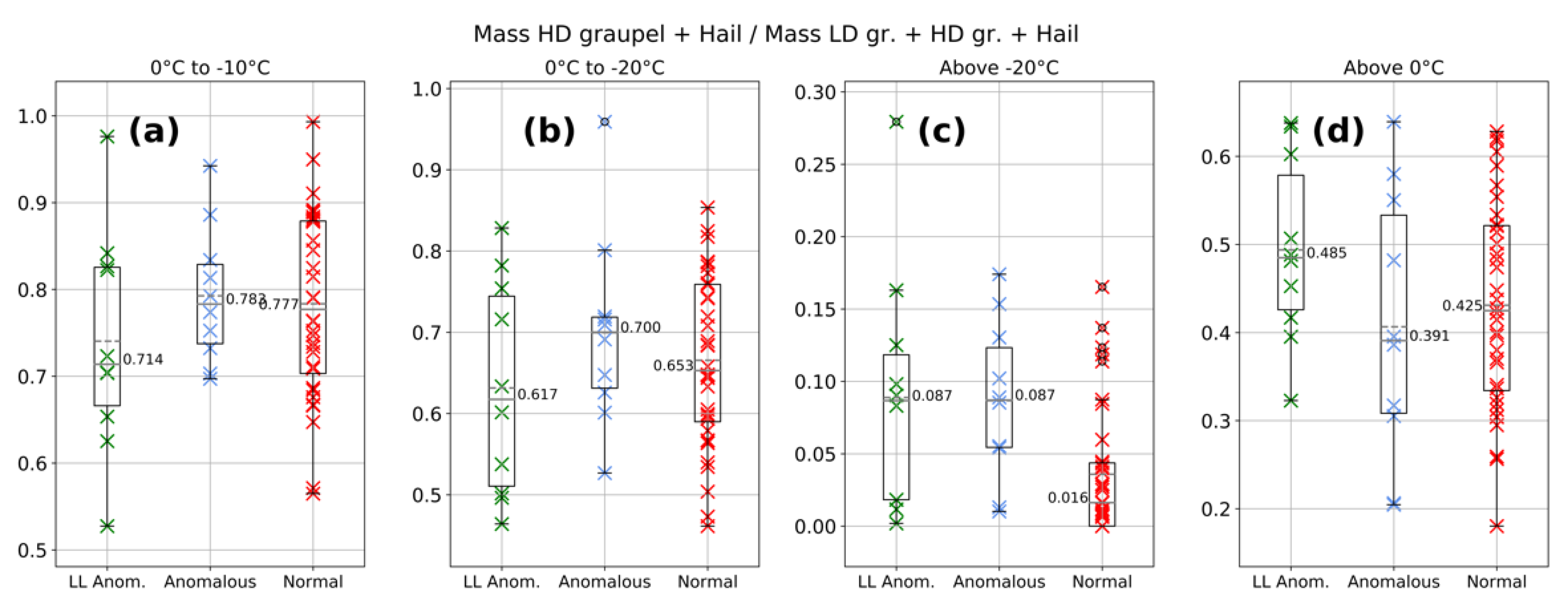
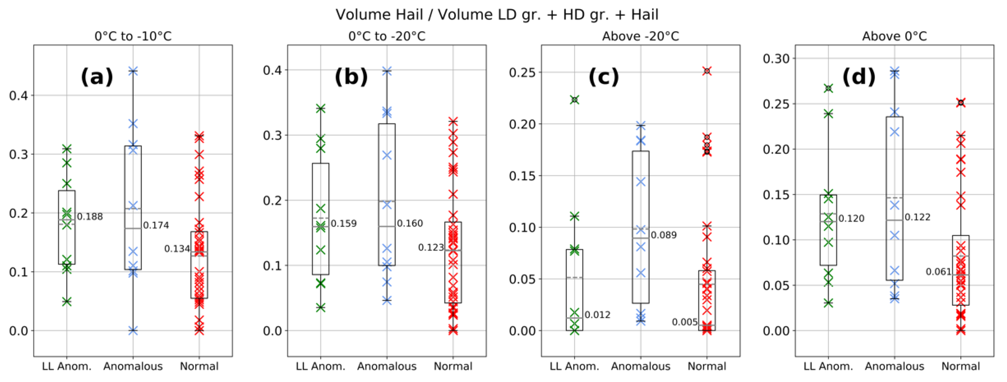
Anomalous datasets for mass of hail, fraction of hail mass in relation to all rimer particles, and volume of hail presented larger values than low-level anomalous and normal datasets, most of them with high statistical confidence. When considering high-density graupel together with hail in these parameters, similar results were obtained, but with lower statistical confidence, i.e., the differences between datasets were less clear. Other studies found the co-location of positive charging in the mixed-phase zone associated with rimer particles [75] or ice mass possibly associated with graupel [3]. In this study, hail was found to be a better signature for inferring the presence of high supercooled cloud LWCs than considering high-density graupel together with hail. This finding is consistent with the hypothesis that anomalous storms have higher LWC in the mixed-phase layer, leading to hail growth and positive charging of these and other rimed particles.
Low-level anomalous datasets presented similar values to anomalous datasets, and higher-than-normal values for the following parameters: mass of hail from 0 °C to −10 °C, fraction of mass and volume of hail from 0 °C to −20 °C, fraction of mass of high-density graupel and hail above −20 °C, fraction of volume of hail from 0 °C to −10 °C and above 0 °C, and fraction of volume of high-density graupel and hail above −20 °C and above 0 °C. These results suggest that sufficiently elevated supercooled cloud LWCs charge rimed precipitation in the lower region of the mixed-phase zone for LLA, while for normal storms, lower LWC favors the growth of low-density graupel in the mixed-phase layer, which contributes to negative charging of rimed precipitation. Some parameters indicated LWCs for low-level positive charging for LLA storms. The elevated temperatures also contribute to positive charging of rimer particles in the lower portion of the LLA mixed-phase layer, but elevated LWC increases the magnitude of positive charging to rimer particles [18,20,27].
Anomalous storms presented a higher frequency of high reflectivity values at all altitudes when compared to LLA and normal storms, as displayed in the CFAD analysis. With a similar outcome, Ref. [76] found that Colorado storms with flash rate mode in the mixed-phase layer (anomalous) had higher reflectivity values in this layer. This was an expected result, as higher supercooled cloud LWC contributes to the growth of large hail and positive charging in the mixed-phase layer for these events. LLA storms presented lower frequency of large reflectivities when compared to normal storms due to the shallow nature of these events.
Kinematic proxy parameters showed that LLA storms had weaker updrafts than other charge structure categories. This result is reasonable, because the transport of liquid water from the warm cloud depth to the mixed-phase layer is limited to the lower portion of this zone, contributing to charging of graupel and hail in that region. No strong vertical development occurs for these events, which contributes to limited or absent upper positive charge being developed. Ref. [77] analyzed the environmental conditions in Argentina that contributed to LLA storms, and they also found weak inferred updrafts from the convective available potential energy (CAPE) parameter, although their LLA sample size was small. In [77], no distinction between anomalous and normal storm datasets was found for kinematic proxy parameters indicative of updraft strength using both soundings and reanalysis datasets. Past studies observed that anomalous charge structure storms have stronger updrafts than normal storms [28,78], while for an environmental analysis of storms in Argentina based on radiosonde data, anomalous storms had lower CAPE than normal storms [77]. Kinematic effects shown in this study alongside the results presented in [77] suggest that updrafts are not an important factor for inducing high LWCs in the mixed-phase zone and anomalous storms, but other factors such as dry low-level humidity and shallow warm cloud depth are more crucial in suppressing growth of droplets in the warm cloud depth, leading to more small droplets that can be lifted, contributing to positive charging of rimer particles in the mixed-phase zone, and anomalously charged thunderstorms to develop.
Figure 11 shows the schematics of normal, anomalous, and LLA storms near Cordoba, Argentina, with their main regions of charge, hydrometeors, and updrafts. Concepts explained above such as anomalous storms having larger amounts of cloud supercooled liquid water caused by higher LCL, lower 0 °C height, and shallower warm cloud depth [77], leading to higher precipitation ice mass and positive charging of rimer particles, can be observed. For all charge structure archetypes, rimer particles (graupel and hail) were the main carriers of charge for the lower charge region of the main dipole, while ice crystals were the carriers of charge for the upper charge region of the dipole. Charging on other particles and possible extra charge layers are speculated to be secondary in relation to the main carriers of charge on the two regions of charge.
Due to the unique occurrence of LLA storms in Argentina, their main characteristics are hereby emphasized (Figure 11), with weaker updrafts, and higher LWC in the lower portion of the mixed-phase layer, leading to higher precipitation ice mass and positive charging of rimer particles in this layer compared to normal storms.
The microphysical and kinematic characteristics of LLA events were explored in relation to anomalous and normal storms. As pointed out by [10], this charge structure is uncommon in U.S. storms; hence, continued investigation of these events is justified. In the future, we will perform a careful case study of a well-observed storm with this charge structure that was within the dual-Doppler lobes of mobile radars operating during the RELAMPAGO intensive operational period [58].

Author Contributions

Conceptualization, B.M. and L.C.; methodology, B.M. and L.C.; software, B.M.; validation, B.M.; formal analysis, B.M. and L.C.; investigation, B.M. and L.C.; resources, L.C. and T.L.; data curation, B.M.; writing—original draft preparation, B.M.; writing—review and editing, L.C., W.D. and T.L.; visualization, B.M.; supervision, L.C., W.D. and T.L.; project administration, L.C., W.D. and T.L.; funding acquisition, L.C. and W.D. All authors have read and agreed to the published version of the manuscript.

Funding

This research was funded by National Science Foundation Award AGS 1661785 and NASA MSFC Grant NNM11AA01A. RELAMPAGO LMA funding was provided by the NOAA GOES-R Program and the NASA Lightning Imaging Sensor (LIS) project.

Institutional Review Board Statement

Not applicable.

Informed Consent Statement

Not applicable.

Data Availability Statement

CSAPR2 data are available at http://www.arm.gov/research/campaigns/amf2018cacti (accessed on 14 June 2021). Radiosonde data are available on the NCAR-Earth Observing Laboratory RELAMPAGO archive at https://data.eol.ucar.edu/master_lists/generated/relampago/ (accessed on 11 February 2021). LMA data are available via https://doi.org/10.5067/RELAMPAGO/LMA/DATA101 (accessed on 5 October 2020).

Acknowledgments

We would like to thank the institutions, universities and individuals who contributed to data collection during RELAMPAGO-CACTI. Special thanks to Faculdad de Matematica, Astronomia, Fisica y Computacion (Universidad Nacional de Cordoba), Eldo Avila, Rodolfo Pereyra, Richard Blakeslee, Jeff Burchfield, Matthew Wingo, Steven Goodman, Michael Solomon, Joy Marich, Phillip Bitzer, Jacquelyn Ringhausen, and Lena Heuscher.

Conflicts of Interest

The authors declare no conflict of interest.

Appendix A

Tables with the Mann–Whitney U-statistic p values are shown below.
Table A1. Mann–Whitney U-statistic p values between datasets for mass of hail. p values are bolded if less than or equal to 0.05.
0 °C to −10 °C0 °C to −20 °CAbove −20 °CAbove 0 °C
LLA-Anomalous0.4270.3070.0070.241
Anomalous-Normal0.0490.0390.0120.034
LLA-Normal0.0910.1620.5730.305
Table A2. Same as Table A1 but for mass of high-density graupel and hail.
0 °C to −10 °C0 °C to −20 °CAbove −20 °CAbove 0 °C
LLA-Anomalous0.3450.2120.0260.140
Anomalous-Normal0.1320.1260.0060.096
LLA-Normal0.3050.3180.4940.372
Table A3. Same as Table A1 but for fraction of mass of hail in relation to mass of all rimer particles.
0 °C to −10 °C0 °C to −20 °CAbove −20 °CAbove 0 °C
LLA-Anomalous0.9700.6230.0530.850
Anomalous-Normal0.1500.1070.0220.179
LLA-Normal0.1130.2160.9450.139
Table A4. Same as Table A1 but for fraction of mass of high-density graupel and hail in relation to mass of all rimer particles.
0 °C to −10 °C0 °C to −20 °CAbove −20 °CAbove 0 °C
LLA-Anomalous0.3850.3850.8500.186
Anomalous-Normal0.8000.5140.0050.622
LLA-Normal0.2260.4170.0310.154
Table A5. Same as Table A1 but for fraction of volume of hail in relation to volume of all rimer particles.
0 °C to −10 °C0 °C to −20 °CAbove −20 °CAbove 0 °C
LLA-Anomalous0.7340.6780.0880.850
Anomalous-Normal0.1190.1010.0100.064
LLA-Normal0.1010.1260.7940.060
Table A6. Same as Table A1 but for fraction of volume of high-density graupel and hail in relation to volume of all rimer particles.
0 °C to −10 °C0 °C to −20 °CAbove −20 °CAbove 0 °C
LLA-Anomalous0.1040.2120.2730.273
Anomalous-Normal0.2580.1320.0050.622
LLA-Normal0.4720.6040.0940.050
Table A7. Same as Table A1 but for kinematic proxies.
Echo Top 20 dBZEcho Top 30 dBZZdr Column Max. Altitude
LLA-Anomalous0.0430.0110.094
Anomalous-Normal0.7980.9670.602
LLA-Normal0.001<0.0010.007

References

  1. Carey, L.D.; Rutledge, S.A.; Petersen, W.A. The relationship between severe storm reports and cloud-to-ground lightning polarity in the contiguous United States from 1989 to 1998. Mon. Weather Rev. 2003, 131, 1211–1228. [Google Scholar] [CrossRef]
  2. Carey, L.D.; Rutledge, S.A. Electrical and multiparameter radar observations of a severe hailstorm. J. Geophys. Res. Atmos. 1998, 103, 13979–14000. [Google Scholar] [CrossRef]
  3. Fuchs, B.R.; Rutledge, S.A.; Dolan, B.; Carey, L.D.; Schultz, C. Microphysical and kinematic processes associated with anomalous charge structures in isolated convection. J. Geophys. Res. Atmos. 2018, 123, 6505–6528. [Google Scholar] [CrossRef] [PubMed]
  4. Wiens, K.C.; Rutledge, S.A.; Tessendorf, S.A. The 29 June 2000 supercell observed during STEPS. Part II: Lightning and charge structure. J. Atmos. Sci. 2015, 62, 4151–4177. [Google Scholar] [CrossRef]
  5. Curran, E.B.; Holle, R.L.; López, R.E. Lightning casualties and damages in the United States from 1959 to 1994. J. Clim. 2000, 13, 3448–3464. [Google Scholar] [CrossRef]
  6. Anderson, K. A model to predict lightning-caused fire occurrences. Int. J. Wildland Fire 2002, 11, 163–172. [Google Scholar] [CrossRef]
  7. DeCaria, A.J.; Pickering, K.E.; Stenchikov, G.L.; Ott, L.E. Lightning-generated NOx and its impact on tropospheric ozone production: A three-dimensional modeling study of a Stratosphere-Troposphere Experiment: Radiation, Aerosols and Ozone (STERAO-A) thunderstorm. J. Geophys. Res. Atmos. 2005, 110, D14303. [Google Scholar] [CrossRef]
  8. MacGorman, D.R.; Burgess, D.W. Positive cloud-to-ground lightning in tornadic storms and hailstorms. Mon. Weather Rev. 1994, 122, 1671–1697. [Google Scholar] [CrossRef] [Green Version]
  9. Zipser, E.J.; Cecil, D.J.; Liu, C.; Nesbitt, S.W.; Yorty, D.P. Where are the most intense thunderstorms on Earth? Bull. Am. Meteorol. Soc. 2006, 87, 1057–1072. [Google Scholar] [CrossRef] [Green Version]
  10. Medina, B.L.; Carey, L.D.; Lang, T.J.; Bitzer, P.M.; Deierling, W.; Zhu, Y. Characterizing Charge Structure in Central Argentina Thunderstorms during RELAMPAGO Utilizing a New Charge Layer Polarity Identification Method. Earth Space Sci. 2021, 8, e2021EA001803. [Google Scholar] [CrossRef]
  11. Williams, E.R. Large-scale charge separation in thunderclouds. J. Geophys. Res. Atmos. 1985, 90, 6013–6025. [Google Scholar] [CrossRef]
  12. Williams, E.R. The tripole structure of thunderstorms. J. Geophys. Res. Atmos. 1989, 94, 13151–13167. [Google Scholar] [CrossRef]
  13. Dye, J.E.; Jones, J.J.; Winn, W.P.; Cerni, T.A.; Gardiner, B.; Lamb, D.; Pitter, R.L.; Hallet, J.; Saunders, C.P.R. Early electrification and precipitation development in a small, isolated Montana cumulonimbus. J. Geophys. Res. Atmos. 1986, 91, 1231–1247. [Google Scholar] [CrossRef]
  14. Bruning, E.C.; Weiss, S.A.; Calhoun, K.M. Continuous variability in thunderstorm primary electrification and an evaluation of inverted-polarity terminology. Atmos. Res. 2014, 135, 274–284. [Google Scholar] [CrossRef]
  15. Emersic, C.; Heinselman, P.L.; MacGorman, D.R.; Bruning, E.C. Lightning activity in a hail-producing storm observed with phased-array radar. Mon. Weather Rev. 2011, 139, 1809–1825. [Google Scholar] [CrossRef] [Green Version]
  16. Marshall, T.C.; Rust, W.D.; Stolzenburg, M. Electrical structure and updraft speeds in thunderstorms over the southern Great Plains. J. Geophys. Res. Atmos. 1995, 100, 1001–1015. [Google Scholar] [CrossRef]
  17. Rust, W.D.; MacGorman, D.R. Possibly inverted-polarity electrical structures in thunderstorms during STEPS. Geophys. Res. Lett. 2002, 29, 12-1–12-3. [Google Scholar] [CrossRef]
  18. Takahashi, T. Riming electrification as a charge generation mechanism in thunderstorms. J. Atmos. Sci. 1978, 35, 1536–1548. [Google Scholar] [CrossRef]
  19. Saunders, C.P.R.; Keith, K.W.; Mitzeva, R.P. The effect of liquid water on thunderstorm charging. J. Geophys. Res. Atmos. 1991, 96, 11007–11017. [Google Scholar] [CrossRef]
  20. Saunders, C.P.R.; Bax-Norman, H.; Emersic, C.; Avila, E.E.; Castellano, N.E. Laboratory studies of the effect of cloud conditions on graupel/crystal charge transfer in thunderstorm electrification. Q. J. R. Meteorol. Soc. 2006, 132, 2653–2673. [Google Scholar] [CrossRef]
  21. Berdeklis, P.; List, R. The ice crystal–graupel collision charging mechanism of thunderstorm electrification. J. Atmos. Sci. 2001, 58, 2751–2770. [Google Scholar] [CrossRef] [Green Version]
  22. Pereyra, R.G.; Avila, E.E.; Castellano, N.E.; Saunders, C.P. A laboratory study of graupel charging. J. Geophys. Res. Atmos. 2000, 105, 20803–20812. [Google Scholar] [CrossRef]
  23. Saunders, C.P.R.; Peck, S.L. Laboratory studies of the influence of the rime accretion rate on charge transfer during crystal/graupel collisions. J. Geophys. Res. Atmos. 1998, 103, 13949–13956. [Google Scholar] [CrossRef]
  24. Baker, B.; Baker, M.B.; Jayaratne, E.R.; Latham, J.; Saunders, C.P.R. The influence of diffusional growth rates on the charge transfer accompanying rebounding collisions between ice crystals and soft hailstones. Q. J. R. Meteorol. Soc. 1987, 113, 1193–1215. [Google Scholar] [CrossRef]
  25. Dash, J.G.; Mason, B.L.; Wettlaufer, J.S. Theory of charge and mass transfer in ice-ice collisions. J. Geophys. Res. Atmos. 2001, 106, 20395–20402. [Google Scholar] [CrossRef]
  26. Emersic, C.; Saunders, C.P.R. Further laboratory investigations into the relative diffusional growth rate theory of thunderstorm electrification. Atmos. Res. 2010, 98, 327–340. [Google Scholar] [CrossRef]
  27. Jayaratne, E.R.; Saunders, C.P.R.; Hallett, J. Laboratory studies of the charging of soft-hail during ice crystal interactions. Q. J. R. Meteorol. Soc. 1983, 109, 609–630. [Google Scholar] [CrossRef]
  28. Fuchs, B.R.; Rutledge, S.A.; Bruning, E.C.; Pierce, J.R.; Kodros, J.K.; Lang, T.J.; MacGorman, D.R.; Krehbiel, P.R.; Rison, W. Environmental controls on storm intensity and charge structure in multiple regions of the continental United States. J. Geophys. Res. Atmos. 2015, 120, 6575–6596. [Google Scholar] [CrossRef]
  29. Ziegler, C.L.; MacGorman, D.R.; Dye, J.E.; Ray, P.S. A model evaluation of noninductive graupel-ice charging in the early electrification of a mountain thunderstorm. J. Geophys. Res. Atmos. 1991, 96, 12833–12855. [Google Scholar] [CrossRef]
  30. Braham, R.R., Jr. Some measurements of snow pellet bulk-densities. J. Appl. Meteorol. Climatol. 1963, 2, 498–500. [Google Scholar] [CrossRef]
  31. Locatelli, J.D.; Hobbs, P.V. Fall speeds and masses of solid precipitation particles. J. Geophys. Res. 1974, 79, 2185–2197. [Google Scholar] [CrossRef]
  32. Dolan, B.; Rutledge, S.A.; Lim, S.; Chandrasekar, V.; Thurai, M. A robust C-band hydrometeor identification algorithm and application to a long-term polarimetric radar dataset. J. Appl. Meteorol. Climatol. 2013, 52, 2162–2186. [Google Scholar] [CrossRef]
  33. Ludlam, F.H. The hail problem. Nublia 1958, 1, 13–96. [Google Scholar]
  34. Korolev, A.; McFarquhar, G.; Field, P.R.; Franklin, C.; Lawson, P.; Wang, Z.; Williams, E.; Abel, S.J.; Axisa, D.; Borrmann, S.; et al. Mixed-Phase Clouds: Progress and Challenges. Meteorol. Monogr. 2017, 58, 5.1–5.50. [Google Scholar] [CrossRef]
  35. List, R.; Rentsch, U.W.; Byram, A.C.; Lozowski, E.P. On the aerodynamics of spheroidal hailstone models. J. Atmos. Sci. 1973, 30, 653–661. [Google Scholar] [CrossRef] [Green Version]
  36. Bringi, V.N.; Chandrasekar, V. Polarimetric Doppler Weather Radar: Principles and Applications; Cambridge University Press: Cambridge, UK, 2001. [Google Scholar]
  37. Straka, J.M.; Zrnić, D.S.; Ryzhkov, A.V. Bulk hydrometeor classification and quantification using polarimetric radar data: Synthesis of relations. J. Appl. Meteorol. Climatol. 2000, 39, 1341–1372. [Google Scholar] [CrossRef]
  38. Zrnić, D.S.; Keenan, T.D.; Carey, L.D.; May, P. Sensitivity analysis of polarimetric variables at a 5-cm wavelength in rain. J. Appl. Meteorol. 2000, 39, 1514–1526. [Google Scholar] [CrossRef]
  39. Anderson, M.E.; Carey, L.D.; Petersen, W.A.; Knupp, K.R. C-band dual-polarimetric radar signatures of hail. Electron. J. Oper. Meteorol. 2011, 12, 2011-EJ2. [Google Scholar]
  40. Meischner, P.F.; Bringi, V.N.; Heimann, D.; Höller, H. A squall line in southern Germany: Kinematics and precipitation formation as deduced by advanced polarimetric and Doppler radar measurements. Mon. Weather Rev. 1991, 119, 678–701. [Google Scholar] [CrossRef] [Green Version]
  41. Liu, H.; Chandrasekar, V. Classification of hydrometeors based on polarimetric radar measurements: Development of fuzzy logic and neuro-fuzzy systems, and in situ verification. J. Atmos. Ocean. Technol. 2000, 17, 140–164. [Google Scholar] [CrossRef]
  42. Vivekanandan, J.; Zrnic, D.S.; Ellis, S.M.; Oye, R.; Ryzhkov, A.V.; Straka, J. Cloud microphysics retrieval using S-band dual-polarization radar measurements. Bull. Am. Meteorol. Soc. 1999, 80, 381–388. [Google Scholar] [CrossRef]
  43. Dolan, B.; Rutledge, S.A. A theory-based hydrometeor identification algorithm for X-band polarimetric radars. J. Atmos. Ocean. Technol. 2009, 26, 2071–2088. [Google Scholar] [CrossRef] [Green Version]
  44. Carey, L.D.; Rutledge, S.A. The Relationship between Precipitation and Lightning in Tropical Island Convection: A C-Band Polarimetric Radar Study. Mon. Weather Rev. 2000, 128, 2687–2710. [Google Scholar] [CrossRef] [Green Version]
  45. Deierling, W.; Petersen, W.A.; Latham, J.; Ellis, S.; Christian, H.J. The relationship between lightning activity and ice fluxes in thunderstorms. J. Geophys. Res. Atmos. 2008, 113, D15. [Google Scholar] [CrossRef] [Green Version]
  46. Donaldson, R.J., Jr. Radar reflectivity profiles in thunderstorms. J. Atmos. Sci. 1961, 18, 292–305. [Google Scholar] [CrossRef] [Green Version]
  47. Lakshmanan, V.; Hondl, K.; Potvin, C.K.; Preignitz, D. An improved method for estimating radar echo-top height. Weather Forecast. 2013, 28, 481–488. [Google Scholar] [CrossRef]
  48. Saunders, P.M.; Ronne, F.C. A Comparison between the Height of Cumulus Clouds and the Height of Radar Echoes Received from Them. J. Appl. Meteorol. Climatol. 1962, 1, 296–302. [Google Scholar] [CrossRef] [Green Version]
  49. Vonnegut, B.; Moore, C.B. Giant Electrical Storms. Recent Advances in Atmospheric Electricity; Pergamon Press: New York, NY, USA, 1960; pp. 399–410. [Google Scholar]
  50. Herzegh, P.H.; Jameson, A.R. Observing precipitation through dual-polarization radar measurements. Bull. Am. Meteorol. Soc. 1992, 73, 1365–1376. [Google Scholar] [CrossRef] [Green Version]
  51. Illingworth, A.J.; Goddard, J.W.F.; Cherry, S.M. Polarization radar studies of precipitation development in convective storms. Q. J. R. Meteorol. Soc. 1987, 113, 469–489. [Google Scholar] [CrossRef]
  52. Kumjian, M.R.; Khain, A.P.; Benmoshe, N.; Ilotoviz, E.; Ryzhkov, A.V.; Phillips, V.T.J. The Anatomy and Physics of ZDR Columns: Investigating a Polarimetric Radar Signature with a Spectral Bin Microphysical Model. J. Appl. Meteorol. Climatol. 2014, 53, 1820–1843. [Google Scholar] [CrossRef]
  53. Snyder, J.C.; Ryzhkov, A.V.; Kumjian, M.R.; Khain, A.P.; Picca, J. A ZDR Column Detection Algorithm to Examine Convective Storm Updrafts. Weather Forecast. 2015, 30, 1819–1844. [Google Scholar] [CrossRef]
  54. Tuttle, J.D.; Bringi, V.N.; Orville, H.D.; Kopp, F.J. Multiparameter radar study of a microburst: Comparison with model results. J. Atmos. Sci. 1989, 46, 601–620. [Google Scholar] [CrossRef] [Green Version]
  55. Hardin, J.; Hunzinger, A.; Schuman, E.; Matthews, A.; Bharadwaj, N.; Varble, A.; Johnson, K.; Giangrande, S. C-Band Scanning ARM Precipitation Radar (CSAPR2CFRPPIQC); Atmospheric Radiation Measurement (ARM) User Facility: Los Alamos, NM, USA, 2018. [Google Scholar] [CrossRef]
  56. Kollias, P.; Bharadwaj, N.; Clothiaux, E.E.; Lamer, K.; Oue, M.; Hardin, J.; Isom, B.; Lindenmaier, I.; Matthews, A.; Luke, E.P.; et al. The ARM Radar Network: At the Leading-edge of Cloud and Precipitation Observations. Bull. Am. Meteorol. Soc. 2019, 101, E588–E607. [Google Scholar] [CrossRef] [Green Version]
  57. Varble, A.C.; Nesbitt, S.W.; Salio, P.; Hardin, J.C.; Bharadwaj, N.; Borque, P.; DeMott, P.J.; Feng, Z.; Hill, T.C.; Marquis, J.N.; et al. Utilizing a storm-generating hotspot to study convective cloud transitions: The CACTI experiment. Bull. Am. Meteorol. Soc. 2021, 102, E1597–E1620. [Google Scholar] [CrossRef]
  58. Nesbitt, S.W.; Salio, P.V.; Avila, E.; Bitzer, P.; Carey, L.; Chandrasekar, V.; Deierling, W.; Dominguez, F.; Dillon, M.E.; Garcia, C.M.; et al. A storm safari in Subtropical South America: Proyecto RELAMPAGO. Bull. Am. Meteorol. Soc. 2021, 102, E1621–E1644. [Google Scholar] [CrossRef]
  59. Hardin, J.; Hunzinger, A.; Schuman, E.; Matthews, A.; Bharadwaj, N.; Varble, A.; Johnson, K.; Giangrande, S. Cacti Radar b1 Processing: Corrections, Calibrations, and Processing Report. 2020. Available online: https://arm.gov/publications/brochures/doe-sc-arm-tr-244.pdf (accessed on 14 June 2021).
  60. Arias, I.; Chandrasekar, V. Cross Validation of the Network of Ground-Based Radar with GPM during the Remote Sensing of Electrification, Lightning, and Mesoscale/microscale Processes with Adaptive Ground Observations (RELAMPAGO) Field Campaign. J. Meteorol. Soc. Jpn. Ser. II 2021, 99, 1423–1438. [Google Scholar] [CrossRef]
  61. Lang, T.J.; Ávila, E.E.; Blakeslee, R.J.; Burchfield, J.; Wingo, M.; Bitzer, P.M.; Carey, L.D.; Deierling, W.; Goodman, S.J.; Medina, B.L.; et al. The RELAMPAGO Lightning Mapping Array: Overview and initial comparison to the Geostationary Lightning Mapper. J. Atmos. Ocean. Technol. 2020, 37, 1457–1475. [Google Scholar] [CrossRef]
  62. Chmielewski, V.C.; Bruning, E.C. Lightning Mapping Array flash detection performance with variable receiver thresholds. J. Geophys. Res. Atmos. 2016, 121, 8600–8614. [Google Scholar] [CrossRef]
  63. Bruning, E.C. Lmatools: Python Code for Working with VHF Lightning Mapping Array Data, 2015. [CrossRef]
  64. Fuchs, B.R.; Bruning, E.C.; Rutledge, S.A.; Carey, L.D.; Krehbiel, P.R.; Rison, W. Climatological analyses of LMA data with an open-source lightning flash-clustering algorithm. J. Geophys. Res. Atmos. 2016, 121, 8625–8648. [Google Scholar] [CrossRef]
  65. Schumacher, R.S.; Hence, D.A.; Nesbitt, S.W.; Trapp, R.J.; Kosiba, K.A.; Wurman, J.; Salio, P.; Rugna, M.; Varble, A.C.; Kelly, N.R. Convective-storm environments in subtropical South America from high-frequency soundings during RELAMPAGO-CACTI. Mon. Weather Rev. 2021, 149, 1439–1458. [Google Scholar] [CrossRef]
  66. UCAR/NCAR–Earth Observing Laboratory. Multi-Network Composite 5 mb Vertical Resolution Sounding Composite; Version 1.3; UCAR/NCAR–Earth Observing Laboratory: Boulder, CO, USA, 2020. [Google Scholar] [CrossRef]
  67. Helmus, J.J.; Collis, S.M. The Python ARM Radar Toolkit (Py-ART), a library for working with weather radar data in the Python programming language. J. Open Res. Softw. 2016, 4, 25. [Google Scholar] [CrossRef] [Green Version]
  68. Ryzhkov, A.V.; Zrnic, D.S. Polarimetric Rainfall Estimation in the Presence of Anomalous Propagation. J. Atmos. Ocean. Technol. 1998, 15, 1320–1330. [Google Scholar] [CrossRef]
  69. Cressman, G.P. An operational objective analysis system. Mon. Weather Rev. 1959, 87, 367–374. [Google Scholar] [CrossRef]
  70. CSU-Radarmet/CSU_RadarTools; CSU Radar Meteorology Group: Fort Collins, CO, USA, 2021; Available online: https://github.com/CSURadarmet/CSU_RadarTools (accessed on 16 June 2021).
  71. Heymsfield, A.J.; Miller, K.M. Water vapor and ice mass transported into the anvils of CCOPE thunderstorms: Comparison with storm influx and rainout. J. Atmos. Sci. 1988, 45, 3501–3514. [Google Scholar] [CrossRef] [Green Version]
  72. Yuter, S.E.; Houze, R.A., Jr. Three-dimensional kinematic and microphysical evolution of Florida cumulonimbus. Part II: Frequency distributions of vertical velocity, reflectivity, and differential reflectivity. Mon. Weather Rev. 1995, 123, 1941–1963. [Google Scholar] [CrossRef]
  73. Medina, B.L.; Carey, L.D.; Amiot, C.G.; Mecikalski, R.M.; Roeder, W.P.; McNamara, T.M.; Blakeslee, R.J. A random forest method to forecast downbursts based on dual-polarization radar signatures. Remote Sens. 2019, 11, 826. [Google Scholar] [CrossRef] [Green Version]
  74. Wilks, D.S. Statistical Methods in the Atmospheric Sciences, 3rd ed.; Academic Press: Cambridge, UK, 2011. [Google Scholar]
  75. Stough, S.M.; Carey, L.D. Observations of anomalous charge structures in supercell thunderstorms in the Southeastern United States. J. Geophys. Res. Atmos. 2020, 125, e2020JD033012. [Google Scholar] [CrossRef]
  76. Fuchs, B.R.; Rutledge, S.A. Investigation of lightning flash locations in isolated convection using LMA observations. J. Geophys. Res. Atmos. 2018, 123, 6158–6174. [Google Scholar] [CrossRef]
  77. Medina, B.L.; Carey, L.D.; Lang, T.J.; Bitzer, P.M.; Deierling, W. The Relation of Environmental Conditions with Charge Structure in Central Argentina Thunderstorms. Earth Space Sci. 2022, 9, e2021EA002193. [Google Scholar] [CrossRef]
  78. Carey, L.D.; Buffalo, K.M. Environmental control of cloud-to-ground lightning polarity in severe storms. Mon. Weather Rev. 2007, 135, 1327–1353. [Google Scholar] [CrossRef] [Green Version]
Figure 1. Charge layers estimated from lightning flashes using the Chargepol method for (a) a normal charge structure event on 17 December 2018 from 174503 to 175124 UTC, (c) an anomalous event on 14 December 2018 from 001504 to 002124 UTC, and (e) a low-level anomalous event on 5 December 2018 from 193003 to 193623 UTC. Each red (blue) vertical line represents a positive (negative) charge layer estimated from a lightning flash. (b,d,f) Histograms of probability density for positive (red) and negative (blue) charge layers detected from flashes for each storm. The 0 °C and the −10 °C isotherm heights are displayed in the histogram plots.
Atmosphere 13 01329 g001
Figure 2. Mass of hail values in kg and box plots for low-level anomalous (green), anomalous (blue), and normal (red) storms for (a) 0 °C to −10 °C, (b) 0 °C to −20 °C, (c) above the height of the −20 °C isotherm, and (d) above the height of the 0 °C isotherm. Mean values are shown as gray dashed lines, and median values as gray horizontal continuous lines along with its numerical value.
Atmosphere 13 01329 g002
Figure 3. Mass of high-density graupel and hail in kg and box plots for low-level anomalous (green), anomalous (blue), and normal (red) storms for (a) 0 °C to −10 °C, (b) 0 °C to −20 °C, (c) above the height of the −20 °C isotherm, and (d) above the height of the 0 °C isotherm. Mean values are shown as gray dashed lines, and median values as gray horizontal continuous lines along with its numerical value.
Atmosphere 13 01329 g003
Figure 4. Fraction of mass of hail in relation to total rimer mass and box plots for low-level anomalous (green), anomalous (blue), and normal (red) storms for (a) 0 °C to −10 °C, (b) 0 °C to −20 °C, (c) above the height of the −20 °C isotherm, and (d) above the height of the 0 °C isotherm. Mean values are shown as gray dashed lines, and median values as gray horizontal continuous lines along with its numerical value.
Atmosphere 13 01329 g004
Figure 5. Fraction of mass of high-density graupel and hail in relation to total rimer mass and box plots for low-level anomalous (green), anomalous (blue), and normal (red) storms for (a) 0 °C to −10 °C, (b) 0 °C to −20 °C, (c) above the height of the −20 °C isotherm, and (d) above the height of the 0 °C isotherm. Mean values are shown as gray dashed lines, and median values as gray horizontal continuous lines along with its numerical value.
Atmosphere 13 01329 g005
Figure 6. Fraction of volume of hail in relation to total rimer volume and box plots for low-level anomalous (green), anomalous (blue), and normal (red) storms for (a) 0 °C to −10 °C, (b) 0 °C to −20 °C, (c) above the height of the −20 °C isotherm, and (d) above the height of the 0 °C isotherm. Mean values are shown as gray dashed lines, and median values as gray horizontal continuous lines along with its numerical value.
Atmosphere 13 01329 g006
Figure 7. Fraction of volume of high-density graupel and hail in relation to total rimer volume and box plots for low-level anomalous (green), anomalous (blue), and normal (red) storms for (a) 0 °C to −10 °C, (b) 0 °C to −20 °C, (c) above the height of the −20 °C isotherm, and (d) above the height of the 0 °C isotherm. Mean values are shown as gray dashed lines, and median values as gray horizontal continuous lines along with its numerical value.
Atmosphere 13 01329 g007
Figure 8. Average CFADs for (a) LLA, (b) anomalous, and (c) normal events. White contour lines show the difference between events equal to zero (compare it with features shown in Figure 9).
Atmosphere 13 01329 g008
Figure 9. Average CFAD differences between (a) LLA and anomalous, (b) anomalous and normal, and (c) normal and LLA.
Atmosphere 13 01329 g009
Figure 10. Values and box plots for LLA (green), anomalous (blue), and normal (red) storms for (a) echo top height of 20 dBZ, (b) echo top height of 30 dBZ, and (c) maximum altitude of a Zdr column above 0 °C, all units in km. Mean values are shown as gray dashed lines, and median values as gray horizontal continuous lines along with its numerical value. Size of Xs is proportional to the number of observations, with the smallest size being one and largest size being eight observations.
Atmosphere 13 01329 g010
Figure 11. Schematic figure with main regions of charge (+ and − signs), hydrometeors, isotherm heights, and updrafts (arrows) for normal, anomalous, and low-level anomalous charge structure storms.
Atmosphere 13 01329 g011
Publisher’s Note: MDPI stays neutral with regard to jurisdictional claims in published maps and institutional affiliations.

