A Coverage Sampling Path Planning Method Suitable for UAV 3D Space Atmospheric Environment Detection

Abstract

Air pollution affects people’s life and health, and controlling air pollution requires the collection of polluting gas information. Unmanned aerial vehicles (UAVs) have been used for environmental detection due to their characteristics. However, the limitation of onboard energy sources of UAVs will limit the coverage of the detection area and the number of gas samples collected, which will affect the assessment of pollution levels. In addition, to truly and completely reflect the distribution of atmospheric pollutants, it is necessary to sample the entire three-dimensional space. This paper proposes a three-dimensional space path planning method suitable for UAV atmospheric environment detection, which can generate a full-coverage path with optimal coverage density under energy constraints. Simulation results show that the proposed method can effectively improve the coverage density compared with other path generation methods. Field experiments show that the proposed method is reliable and accurate in the application of UAV atmospheric environment space detection.

1. Introduction

In recent years, the process of industrialization and urbanization has been accelerating, but the problems of air pollution and climate change are becoming more and more prominent, seriously affecting people’s daily life and physical health [1,2,3]. The control and traceability of air pollution require the collection of information on polluting gases [4,5]. Commonly used air pollutant monitoring equipment is mainly divided into base station air quality monitoring stations and portable air-quality monitors [6,7]. However, the former has poor flexibility and low coverage density, while the latter has a small measurement range, is limited by the measurement environment, and requires large labor costs [8]. The quadrotor is a powered autonomous aircraft that relies on the sensors and micro-control units it carries for flight control, data acquisition and information processing. It is widely used in many fields, such as photogrammetry, search and rescue missions, farmland monitoring, fire monitoring, military detection and power line inspection detection. In environmental monitoring [9], it can be used as a carrier to carry a gas sensing device to complete the collection of pollution information in three-dimensional space for specific polluted areas, such as industrial parks, sewage treatment plants, etc.

In order to obtain environmental information, mobile sensing robots equipped with gas sensors must navigate to sampling locations in the monitored area to make the necessary measurements, and higher resolution sampling covering the entire space will obviously provide real data closer to underlying environmental phenomena. However, UAVs in this field have limited onboard energy, which limits the number of data samples collected and the associated coverage. In related literature, this determination of an optimal path involving all points in a given region of interest is often referred to as the Coverage Path Planning problem (CPP). In previous work, most UAVs flew in a “Z” or lawnmower mode at a single altitude during CPP missions and did not consider whether the robot had enough power to cover the entire area. In an atmospheric environment detection mission, because the distribution of different gases at different heights is different [10,11], it is necessary for the UAV to perform a large amount of data measurement of the entire space, rather than a single height plane. Peng [12] uses a pyramid-shaped spiral flight path for atmospheric environment detection. While it can collect gas data at different altitudes, it can only collect data from space boundary points and cannot fully cover samplings from the space region, and therefore cannot reconstruct the gas distribution throughout the three-dimensional space.

CPPs can be divided into two categories [13] according to the way the regions are decomposed. One type is called grid-based decomposition, which discretizes the coverage area into a grid and then plans a path to visit each grid cell. Another type is called cell decomposition, which divides the coverage area into different units as needed. These units are then overlaid with a zig-zag flight, and finally the traveling salesman problem on adjacent decomposition units is solved to determine the sequence of access units. Methods based on grid decomposition include a spiral spanning tree [14], a wavefront algorithm based on distance transforms and an adaptive D* path planning method [15]. These methods decompose the area that needs to be covered into grid cells, such as triangles, squares [16], and hexagons, and then sample these grid cells. This paper uses this idea; the difference is that we use the hexagonal prism as the basic unit, and then use the center of the unit as the sampling point, so as to collect data samples with balanced spatial distribution in the entire study area, rather than only the data of a certain height plane. When planning access paths for grid cells, the traveling salesman problem (TSP) [17] is widely used by directly connecting all target locations. It finds the path by visiting each location exactly once, and provides the shortest path for mobile awareness. Jimenez [18] proposed a genetic algorithm with path templates to obtain paths. Of course, there are other methods. Nam [19] obtained the coverage path according to the region of interest marked by the wavefront and proposed a task execution time optimization criterion based on the length of the path. There are many CPP methods based on cell decomposition, such as boustrophedon decomposition [20], Morse decomposition [21], lawn mower path [22] and its variants [23]. Boustrophedon cell decomposition solves the problem of covered areas with known obstacles by decomposing the target area under the obstacle location and then finding the least costly route through all areas [24]. Yildirim [25] proposed an improved cell decomposition algorithm to improve the complete coverage efficiency of autonomous environmental monitoring systems. Bahnemann [26] optimized Boustrophedon coverage by using several scanning methods and combining them according to the required transition motion between obstacles and cells, and some extensions of the algorithm also took sensor feedback into account [27].

The reference [28] details how to plan a full coverage path, but most planners do not consider the energy constraints of UAVs, nor do they address or emphasize the limited total travel length. Only recently have researchers begun to consider energy constraints in full-coverage path planning [29,30,31]. Li [32] determined the total length of the voyage according to the energy limit in his work, and constructed a scalar map of monitoring parameters to assess the performance of coverage sampling. Cabreira [31] treated camera characteristics as image resolution and field of view, avoiding moving over already visited areas, and proposed an energy-aware spiral coverage path planning algorithm designed for optics. Jensen-Nau [33] proposed a dynamic path model consisting of a chained mass-spring-damper system combined with a Voronoi diagram to generate a potential field in which pre-connected path waypoints are distributed to distribute the path waypoints into a near-optimal configuration. However, it may not be optimal to address the energy shortage in planning only by limiting the total travel length. In Modare’s work [29], two main factors affecting the UAV’s energy consumption were identified through experimental measurements: distance and cornering. They found that the average power consumption of the UAVS is almost constant during flight, but when entering a turn, it typically decelerates sharply, even to zero to hover steering, leading to longer flight times and increased energy consumption.

In this paper, a UAV-based mobile sensing sampling path planning method for spatial sampling of the atmospheric environment is proposed, which integrates spatial coverage sampling design and related path planning. Based on the sampling design of the hexagonal prism, the sampling space is divided into subregions of the same size, and the sampling point is the center of the hexagonal prism. A Genetic Algorithm is used to solve the sampling path. Combined with the energy budget of UAVs, the optimum coverage density can be obtained by adjusting the side length of the hexagonal prism. by improving the genetic algorithm and combining the B-spline curve to optimize the flight path, the number of turns of the path and the speed loss of the UAV during turning are effectively reduced, and the coverage performance and data sampling density of the atmospheric environment detection missions are improved. The rest of the paper is organized as follows. Section 2 details the coverage sampling design and path planning methods. Section 3 presents the simulation and field experiments, and discusses the experimental results. The final section concludes the paper.

2. Materials and Methods

2.1. Sampling Design

To obtain the fine-grained distribution of air pollution in the detection area and to reflect the pollution status of the area to the greatest extent, the sampling points need to cover the entire space area. Considering the cruising range of the UAV, the number of sampling points needs to be limited. Therefore, it is necessary to select the appropriate number of sampling points within the range of a UAV cruise and to distribute the sampling points as evenly as possible in the detection space to improve detection coverage.

During an atmospheric environment detection mission, the study area A (space of interest) is decomposed using the hexagonal prism unit to generate points of interest covering sampling, and then the sampling path is mapped. As shown in Figure 1, the basic decomposition unit is a regular hexagonal prism with a height of $\sqrt{3}L$; its base is a regular hexagon with a side length of L and the six side edges are perpendicular to the base. The entire study area is uniformly decomposed by the basic unit of the hexagonal prism. In the vertical direction, the space of interest is divided into subspace regions of interest with the same height. The basic unit whose centroid is in the study area is called the sub-region of interest, and these centroids are the sampling locations used to collect data samples. For a given study area and L, the number N of decomposed subspace regions of interest, the set M of sub-region of interest in a single subspace and their number |M| can be obtained. When the UAV collects environmental data, the navigation path requires access to each sub-region of interest. Suppose the planned path is P and the path length is |P|, as shown in Formula (1).

$$\begin{array}{c}\begin{array}{cc}P=\left\{s_1,s_2\dots s_n\right\}& s_n\in M,n=1,2\dots N\left|M\right|\end{array}\hfill \end{array}$$

(1)

where $s_n$ represents the sampling location (waypoint) visited in path P.

2.2. Optimal Coverage Sampling Density

After the basic unit decomposition, the study space is divided evenly into sub-regions of the same size. One basic unit is a sub-region and the sampling position is its centroid. At this time, the distance between any two adjacent sub-regions of interest is equal, and the spatial sampling coverage density can be represented by this distance. Given the space and L, the spatial sampling coverage density $d=\sqrt{3}L$ and the length $\left|P\right|=d\ast (N\left|M\right|-1)$ of the generated path P can be preliminarily determined. Since the average power consumption of the UAV is almost constant during flight, we assume that the power consumption of the UAV follows the linear model $f\left(P\right)=u_e\ast \left|P\right|$, where $u_e$ is a constant control parameter, representing the energy consumption per unit length of the UAV, and $f\left(P\right)$ is the energy consumption in the path P. By adjusting the size of L, the number |M| of sub-regions of interest in the study area can be intuitively increased or decreased, and the size of |P| can be controlled. Combined with the energy budget $E_{dbt}$, the optimal parameter $L^{*}$ and the largest |M| can be found, such that the resulting coverage path has the densest coverage sampling. The optimal spatial coverage density $d^{*}$ is determined by $L^{*}$, as shown in Formula (2):

$$\begin{array}{c}{\mathrm{d}}^{*}=\sqrt{3}{L}^{*}=\underset{L}{arg max}\left|M\right|\hfill \\ \begin{array}{cc}s.t.& f\left(p\right)=u_e·\left|P\right|<E_{dbt}\end{array}\hfill \end{array}$$

(2)

2.3. Coverage Path Planning

In order to achieve full coverage sampling of the region, when planning a path, we first generate an ordered sequence of all sub-regions of interest, and the sequence represents the access order of sub-regions of interest. The coverage path is generated based on this sequence, and the UAV flies according to the path and sequentially visits each sub-region of interest to perform gas sampling operations. The Genetic Algorithm is an algorithm commonly used to solve the TSP problem in UAV path planning research [34]. It is a random global search algorithm proposed according to the theory of “survival of the fittest” in evolution theory [35], which uses coding techniques to transform optimization problems in practical fields into strings of chromosomal data. One chromosome corresponds to one possible solution. Then, according to the process of biological evolution in nature, excellent solutions are selected for genetic variation; that is, iterative optimization.

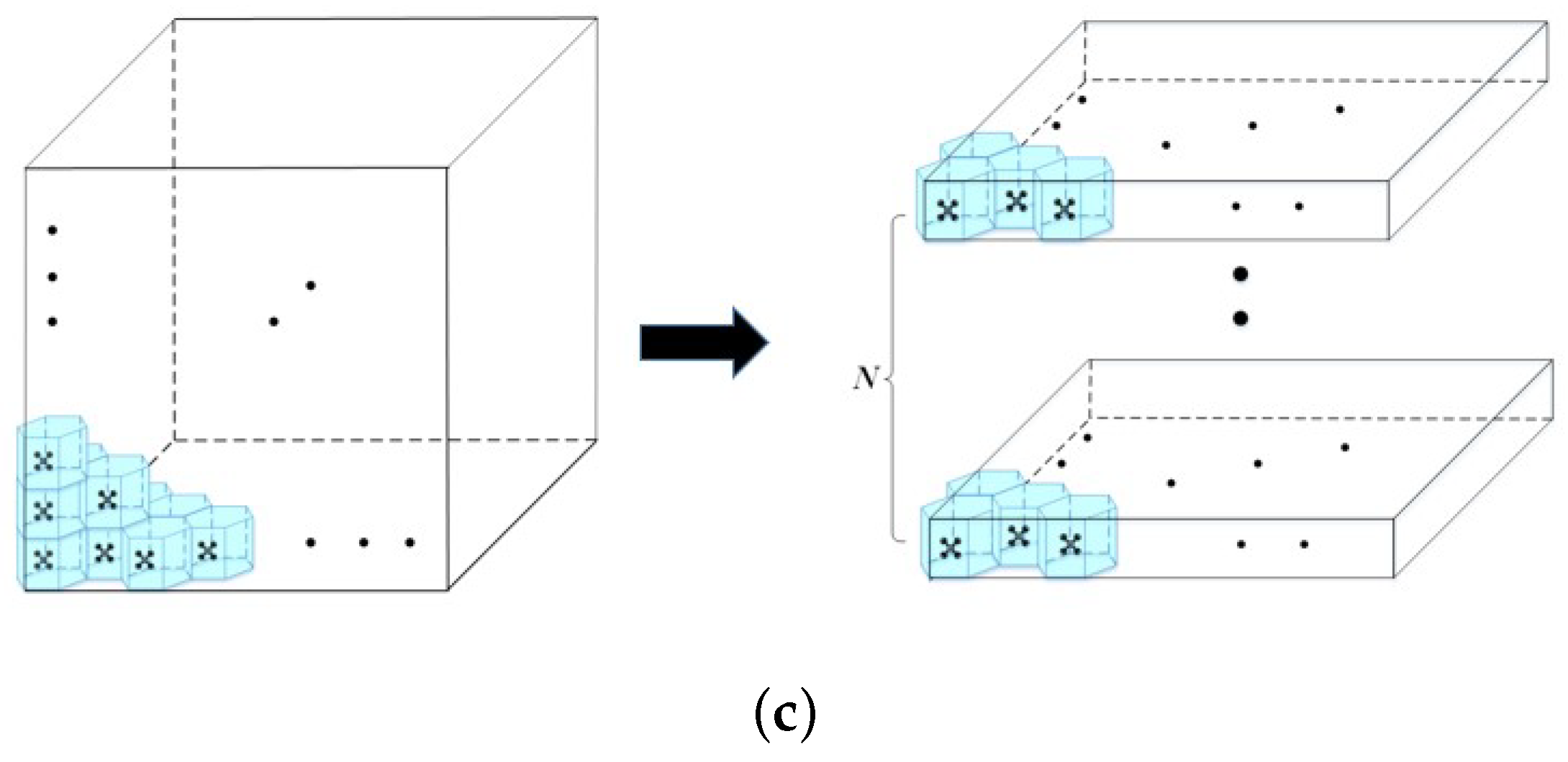
In this study, we decompose the entire study area from both horizontal and vertical perspectives, resulting in more path points than the traditional CPP algorithm. The TSP solver is non-terminal polynomial-time hard (NP-hard), and the more waypoints it takes, the more time it takes to compute. To solve this problem, we transform the path of an entire space into a path with only one interested subspace, and obtain the path of its adjacent subspace by searching for the inverse order of the path points, since the entire space is uniformly decomposed, the number of the sub-region of interest in each subspace is the same and the coordinate positions are the same except for the height. To solve this problem, we transform the path of an entire space into a path with only one interested subspace, and obtain the path of its adjacent subspace by searching for the inverse order of the path points, since the entire space is uniformly decomposed, the number of the sub-region of interest in each subspace is the same, and the coordinate positions are the same except for the height. In order to quickly plan the optimal detection path suitable for the detection task, this paper improves the population initialization method, fitness function and genetic operator based on the traditional genetic algorithm.

2.3.1. Coding

Using the genetic algorithm to solve the problem, the possible solutions to the problem need to be encoded first. Traditional optimization problems mostly use binary coding, but the chromosomes in a point planning problem are composed of subregions of interest (sampling points), so coding based on the sampling point number is sufficient and more in line with the reality of the problem. For example, a detection task has a total of seven sampling points, which can be represented by the sampling point set $P=\left\{p_i\right|i=1,2,···7\}$, then a possible solution (chromosome) of the waypoint planning problem is $p_2-p_4-p_1-p_6-p_7-p_3-p_5$, where each code (gene) represents a sampling point.

2.3.2. Population Initialization

Population initialization is more important, and it will affect whether the genetic algorithm can converge to the global optimal solution. In the case of many waypoints, the quality of the randomly generated initial population may be low, requiring too many iterations to obtain the optimal solution. Therefore, we use the nearest neighbor path as the initial population. After randomly selecting the first path point, we select the sample point closest to the current path point as the next waypoint to generate the nearest neighbor path.

2.3.3. Design of Fitness Function

The fitness function can judge the superiority and inferiority of individuals in a population, and has a great influence on the efficiency of the genetic algorithm in searching for optimal solutions. In traditional genetic algorithms, the path length is often used as the fitness function [36]. In this study, the total length of the path and the number of turns were considered from the point of view of minimizing energy loss. Aiming at the problems existing in the traditional fitness function, an improved dynamic fitness function is proposed to evaluate the length of the planned path and the turning angle of the connecting points in the path. The improved functions are as follows in Formula (3):

$$\begin{array}{c}fitness=\frac{1}{a_{1}S+a_2{\displaystyle \sum _{i=1}^{N\left|M\right|-2}}{\theta }_i}\hfill \end{array}$$

(3)

where S is the path length, determined by the Formula (4), ${\theta }_i$ is the steering angle from the i waypoint to the $i+1$ waypoint turning to the $i+2$ waypoint, as shown in Figure 2.

$$\begin{array}{c}S={\displaystyle \sum _{i=1}^{N\left|M\right|-1}}∥p_{i+1}-p_i∥\hfill \end{array}$$

(4)

$p_{\mathrm{i}}\in M$ is the waypoint on the flight path, $∥p_{i+1}-p_i∥$ is the Euclidean distance between two adjacent waypoints on the flight path.

$a_1$ and $a_2$ are weight coefficients, usually fixed constants. In this paper, they represent the influence of path length and steering angle, which determine the convergence direction of the algorithm. Throughout the flight sampling process, the flight distance consumes far more energy than the turning, and the shortest path is known in advance. In order to ensure that the iterative result satisfies the shortest path first, the algorithm preferentially converges to the shortest path during iteration by dynamically adjusting $a_1$ and $a_2$. When the number of individuals with the shortest path in a population reaches a certain critical value, the influence of steering angle increases. The specific formula is as follows (5).

$$\begin{array}{c}\begin{array}{c}{a}_1=\left\{\begin{array}{cc}{a}_{ max}-\frac{a_{ max}-a_{ min}}{n_{ max}-n_0}(n-n_0)& n>n_0\\ a_{ max}& n\le n_0\end{array}\right.\hfill \\ a_1+a_2=1\hfill \end{array}\hfill \end{array}$$

(5)

In the formula, $a_{ max}$ and $a_{ min}$ are the maximum and minimum values of $a_1$, n is the number of individuals with the shortest path in the current population, $n_0$ is the minimum critical value and $n_{ max}$ is the maximum critical value. $a_1$ is $a_{ max}$ before n is smaller than $n_0$, making the convergence direction more inclined towards the shortest path.

2.3.4. Genetic Operator Improvement

Genetic operation is divided into three parts: selection, crossover and variation, which is the core of the Genetic Algorithm. In order to determine the algorithm converge quickly and improve the planning speed, we optimize the selection operation. Before the roulette selection method selects individuals from the population for genetic operation, we sort each individual according to the fitness from high to low, select the good individuals with high fitness as the excellent population according to a certain proportion, and then use the roulette method to select individuals from the excellent population for genetic manipulation. However, this step will reduce the diversity of the population and may cause the algorithm to fall into a local optimum. Therefore, we use adaptive adjustment of the crossover operator and mutation operator and introduce a selection operator to jump out of the local optimum, so that the population as a whole maintains high fitness and evolves to higher fitness, as follows in Formulas (6)–(8).

$$\begin{array}{c}{P}_r=P_{r max}-\frac{P_{r max}-P_{r min}}{t_{ max}}t\hfill \end{array}$$

(6)

$$\begin{array}{c}{P}_c=P_{c max}-\frac{P_{c max}-P_{c min}}{t_{ max}}t\hfill \end{array}$$

(7)

$$\begin{array}{c}{P}_m=P_{m min}+\frac{P_{m max}-P_{m min}}{t_{ max}}t\hfill \end{array}$$

(8)

In the formula: $P_r$ is the selection retention ratio of excellent individuals, $P_{r max}$ and $P_{r min}$ are the maximum and minimum selection retention ratios of excellent individuals, respectively; $P_c$ is the crossover probability, $P_{c max}$ and $P_{c min}$ are the maximum and minimum crossover probability, respectively; $P_m$ is the mutation probability, $P_{m max}$ and $P_{m min}$ are the maximum and minimum mutation probability, respectively; $t_{ max}$ is the maximum number of iterations; and t is the current iteration algebra.

In the early stage of algorithm iteration, the population is quite different, rich in species and has good diversity. Selecting a larger retention ratio of excellent individuals and crossover probability can retain a richer variety of individual types and evolve new high-quality individuals at the same time. A lower mutation probability can reduce the possibility of good individuals being destroyed and increase the speed of convergence. In the later stage of iteration, the fitness of individuals in the population is concentrated, and the degree of difference is small. Reducing the retention ratio of excellent individuals and crossover probability and increasing the mutation probability can prevent the algorithm from falling into local extreme values and can search for the global optimal solution.

2.3.5. Algorithm Simulation

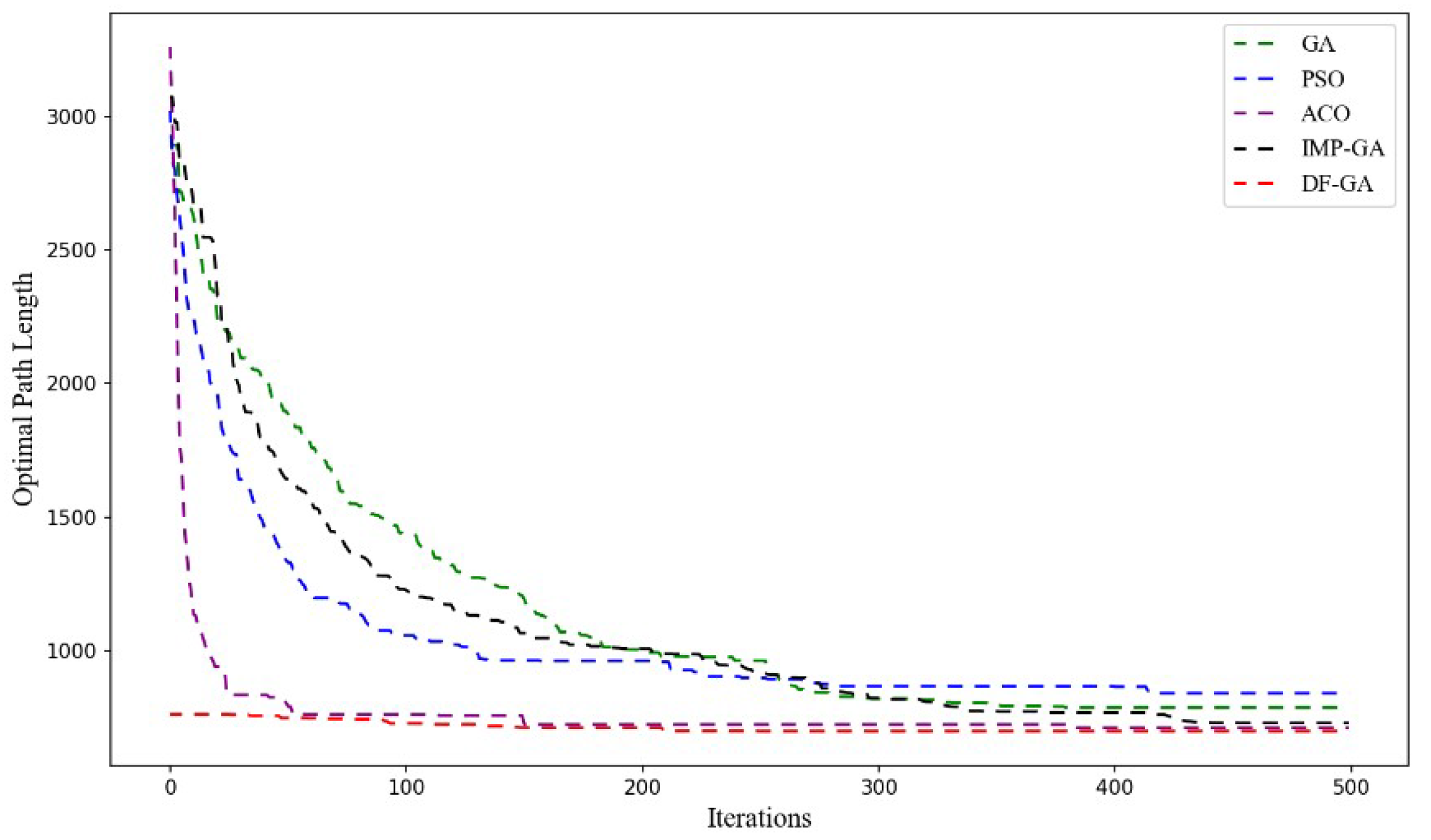
Based on the above improvements, the st70 dataset is used for validation. st70 is a dataset in the problem library TSPLIB of TSP and related problems; it contains 70 cities and their coordinate information, with an optimal path distance of 675. We use the dynamic adaptive function genetic algorithm (DF-GA) in this paper to compare and verify the algorithm with traditional genetic algorithm (GA), particle swarm optimization (PSO), ant colony optimization (ACO), and improved Genetic Algorithm (IMP-GA) [37]. Each algorithm was repeated 50 times, recording the convergence algebra and convergence value of each algorithm. The convergence curve is shown in Figure 3. At the same time, the average convergence iteration times, average convergence value and average convergence time of 50 experiments of each algorithm are calculated, and the results are shown in

Table 1. The performance of different algorithms on the st70 dataset.

Algorithm	Average Path Length (m)	Average Count of Iterations (Count)	Average Convergence Time (s)
GA	744.73	432.25	9.13
PSO	797.09	442.61	20.61
ACO	718.98	361.50	68.34
IAM-GA	738.39	417.93	21.00
DF-GA	699.04	248.35	4.32

. Note that here, the DF-GA only includes the improvement of the population initialization and the genetic operators, not improving the fitness function, as the test dataset does not consider the angle information.

As can be seen from Figure 3, the DF-GA has a better initial population and the convergence value is significantly lower than other algorithms. Combined with Table 1, our algorithm solves an average path of 699.04, which is only 3.44% different from the optimal path of 675. Compared to GA, PSO, ACO, and IMP-GA, path lengths are reduced by 6.14%, 12.30%, 2.77%, and 5.33%, respectively, significantly, and reduce convergence iteration algebra and convergence time. The results show that our Genetic Algorithm can obtain a better path in a shorter time, has fewer iterations, and can effectively avoid falling into local optimization.

In order to evaluate the performance of the algorithm after adding angle parameters to the adaptation function and dynamically adjusting the weights, we use the algorithm (DF-GA) in this paper, the algorithm in this paper with fixed weight coefficients (SF-GA), and the traditional Genetic Algorithm (GA) without angle parameters to perform path planning for the sampling design above. We performed 30 repeated experiments for each algorithm, the number of iterations was set to 500, and the relevant data in the experiment were recorded, as shown in

Table 2. Performance of different Genetic Algorithms in solving paths in study area A.

Algorithm	Optimal Path Length (m)	Optimal Angle (Rad)	Average Path Length (m)	Average Angle (Rad)	Average Count of Iterations (Count)
GA	472.85	96.34	476.08	112.76	343.52
SF-GA	472.85	87.96	474.75	98.28	407.27
DF-GA	472.85	85.87	474.75	96.13	393.35

.

It can be seen from Table 2 that the shortest path can be obtained by all three algorithms, but the dynamic and static algorithm are superior to the traditional genetic algorithm in terms of optimal angle and total average angle, which shows that increasing angle parameters can effectively reduce the number of turns of the path. The dynamic function algorithm is better than the static in terms of total average angle and optimal angle, which shows that dynamic adjustment weight is effective. The traditional function is superior in iteration numbers because it does not consider angle constraints. The dynamic function is still superior to the static function when angle constraint is considered. Figure 4 are the paths planned by the traditional genetic algorithm and dynamic function genetic algorithm, respectively. The angle of (a) is 114.14 and that of (b) is 92.15. It can also be seen from the figure that path (b) consists of more straight sections with fewer turns than (a).

2.4. Curve Fitting

By covering sampling design and genetic algorithm, the detection path with the optimal sampling resolution can be obtained under the energy limitation. However, this path does not meet the requirement of the continuous flight path of the UAV; that is, the second-order continuous differentiability. As a result, the UAV will decelerate, hover and turn at some discontinuous waypoints during the flight, which will increase mission execution time and waste a lot of energy. Path smoothing is an effective method used to obtain the actual flight path of UAVs, which can improve the safety and efficiency of UAVs. The B-spline method retains all the advantages of the Bezier method and overcomes the fact that the Bessel method cannot modify local curves and the complexity of curve splicing. The B-spline function has continuous first and second derivatives, and the curvature change is relatively uniform; it meets the requirements of the continuous change of the speed and acceleration rate of the UAV. When the B-spline curve is used for track smoothing, it can achieve a smooth transition of the intersecting parts of the track, and the B-spline curve can be partially adjusted according to the local adjustment of the track point. The new track obtained is in the convex hull, which ensures that the cost of the new track and the cost of the original track vary within a certain allowable range.

The B-spline curve is a generalized form of the Bezier curve, which is defined as the following Formula (9):

$$\begin{array}{c}\mathrm{C}\left(u\right)={\displaystyle \sum _{i=0}^n}{N}_{i,p}\left(u\right)P_i\hfill \end{array}$$

(9)

where $P_i,i\in [0,n]$ is the control point of the B-spline curve. $N_{i,p}$ is the basic function of the B-spline curve and the subscript p represents the order of the basis function. Compared with the Bezier curve, the B-spline curve introduces the node vector $U=\{u_0,u_1,u_2,\dots ,u_m\},u_0\le u_1\le u_2\le ···\le u_m$, which divides the original $u\in [0,1]$ into multiple node segments. The point $C\left(u_i\right)$ corresponding to the curve on the nodal vector is called a node, so that the entire B-spline curve is divided into many curve segments by the nodes, and each curve segment is actually a P-order Bezier curve defined on the node segment.

The definition of the basis function depends on the nodal vector, which can be obtained according to the recursive definition of De Boor–Cox, as shown in the following Formula (10):

$$\begin{array}{c}\begin{array}{c}{N}_{i,0}\left(u\right)=\left\{\begin{array}{cc}1& u_i\le u<u_{i+1}\\ 0& otherwise\end{array}\right.\hfill \\ N_{i,p}\left(u\right)=\frac{u-u_i}{u_{i+p}-u_i}{N}_{i,p-1}\left(u\right)+\frac{u_{i+p+1}-u}{u_{i+p+1}-u_{i+1}}{N}_{i+1,p-1}\left(u\right)\hfill \end{array}\hfill \end{array}$$

(10)

We use a third-order B-spline curve to smooth the path and find that when the sampling point spacing is too large, the fitted curve will deviate far from the sampling point, so that the path only covers a certain edge of the sub-region of interest. Therefore, we add supplementary waypoint interpolation before using B-spline curve fitting. As shown in Figure 5, before and after the waypoint to be turned, four new waypoints are inserted at d/2 and d/4 distances from the current waypoint, respectively, so that the new path fitted by the B-spline curve approaches the waypoint with the premise of maintaining the original constraints.

The detection path after curve fitting is shown in Figure 6. At this time, the current path distance P can be obtained, and then the optimal coverage sampling density can be obtained by Formula (2).

2.5. Discussion

This section mainly introduces the coverage sampling design and path planning methods. First, the study space is decomposed by basic units to obtain uniformly distributed spatial sampling points. Combined with the UAV energy budget, optimal coverage density can be obtained. We improved the Genetic Algorithm by introducing a dynamically adjusted fitness function and selection operator when solving the sampling path. The simulation results show that the improved algorithm has better performance, which can significantly reduce the computation time and obtain an excellent detection path. Finally, the B-spline curve is used to smooth the path curve, which reduces the energy consumption of the UAV steering and further saves energy.

3. Results and Discussion

3.1. Simulation

AirSim is an unmanned automatic control simulation platform developed by Microsoft. The entire system is based on Unreal Engine 4, with a highly restored physics engine and realistic visual scenes. AirSim supports both software-in-the-loop and hardware-in-the-loop simulation, with sensors such as lidar, camera, IMU, GPS, and more to control drones not only with python and C++ code, but also directly via remote control. Compared with Matlab, Gazebo, FlightGear, and other simulation platforms, AirSim has advantages such as strong 3D rendering, flexible control methods, fine model textures, and strong scalability.

The simulation system, shown in Figure 7, mainly includes the AirSim simulation platform, Pixhawk4 flight controller and UAV ground control station. AirSim is housed in Unreal Engine 4. As the core and hub of the system, it is connected to the Pixhawk4 flight controller through serial ports, to the ground station through UDP, and communicates with each other using the MAVLink protocol. The Pixhawk4 flight controller has PX4 firmware built in. PX4 provides a UAV control model that sends control commands to the UAV fuselage model in AirSim, enabling the UAV to follow algorithm instructions. UAV ground control station can directly control the UAV’s flight and can also set up missions that allow the UAV to fly autonomously. The entire simulation process can obtain information such as flight trajectory, visual image and position status of UAV from the ground station and Unreal Engine 4.

The energy budget determines the total flight time of the UAV. For simplicity, we use the flight time to represent energy consumption in simulations and evaluate the algorithm’s performance by measuring total flight time under different sampling coverage in the same region.

Table 3. Algorithm budgets for different coverage densities in study area A.

Algorithm	L	Path Length	Time
LMP		746.94	523.13
HGC	3.00	472.85	428.85
HGTB		451.29	358.17
LMP		563.57	381.18
HGC	4.00	367.19	304.99
HGTB		352.18	235.05
LMP		433.28	287.69
HGC	5.00	285.79	197.77
HGTB		278.33	169.95

shows the comparison information of the lawnmower path planner (LMP), the auxiliary coarse cell-based hexagonal grid coverage (HGC) sampling planner [29] and the path planner (HGTB) in this paper. Because LMP and HGC are both single-plane covering algorithms, the algorithm in this paper only considers the energy consumption of one subspace region. The lawnmower path can be regarded as a square-based unit division, so the L of the lawnmower path in the table is the side length of the square unit. It can be seen from the table that under the same coverage, HGTB takes less time, which means that with the same energy budget, HGTB can achieve longer flight sampling and obtain spatial sampling data with higher coverage.

3.2. Field Tests

To verify the practical performance of the proposed path planning method, we conduct a one-week outdoor flight test. The tests will be conducted daily between 2:00 and 3:00 at noon from 2 January 2022 to 8 January 2022 at the Western Playground of Hebei University of Technology. As shown in the red zone in Figure 8, the measurement area is a space area of about 80 m × 100 m in size and 20 to 100 m in height. There are traffic lanes around, and the buildings to the southwest are two student canteens. The four-rotor drone used is a ZD550 with a wheelbase of 550 mm and a fuselage made mainly of carbon fiber and metal, with 14-inch carbon fiber propellers. Its tripod and arm are made of hollow carbon fiber tubes, which effectively reduce its weight with the premise of ensuring hardness, with a maximum additional load of 3 kg, using a 10,000 mAh-6S power battery, and the no-load flight time is 30 min. During the test, the rotorcraft flies according to the planned path, as shown in Figure 8b. The airborne gas acquisition device collects gas data at a frequency of two times per second, and the experimental measurement is performed twice a day.

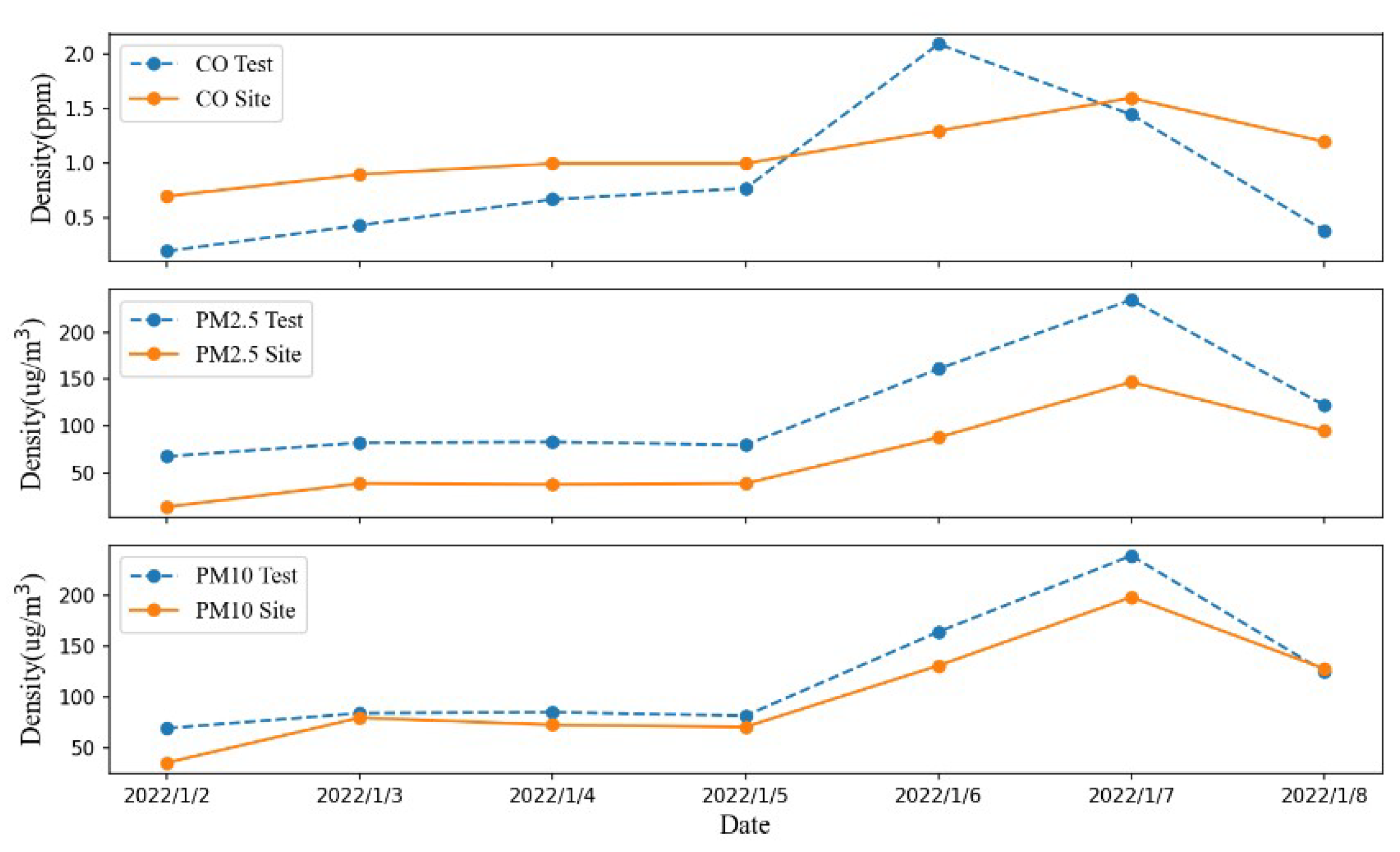
A total of 14 gas data are obtained for the experiment: 2 per day. Each measurement lasts about 20 min, and the measured air pollution components are CO, PM2.5 and PM10. The average value of the measured data for each day was selected as the atmospheric pollution gas concentration on that day, and compared with the daily air quality data released by the Huaihe Road State Control Station of the Tianjin Ecological Environment Monitoring Center (about 10 km away from Hebei University of Technology), As shown in Figure 9. The solid line is the site data, and the dashed line is the experimental result of environmental measurement. Taking mean absolute error (MAE) and root mean square error (RMSE) as evaluation indicators, the smaller the value of the evaluation indicators, the smaller the error. The results are shown in

Table 4. Comparison of evaluation index results.

Index	CO	PM2.5	PM10
MAE	0.47	53.04	19.71
RMSE	0.53	56.38	24.44

.

On the time scale, the results of the pollution gas concentration measured in this experiment are basically consistent with the monitoring results of the Huaihe Road State Control Station. Since there is a certain distance between Hebei University of Technology and the Huaihe Road State Control Station, and the real-time environmental conditions have deviations, the deviation between the experimental results and the results of the State Control Station is within an acceptable range.

We randomly selected one day’s experimental data, used the Kriging interpolation method to interpolate the gas data, and analyzed the distribution of polluted gases in the measurement space. The results of PM2.5 interpolation are shown in Figure 10. It can be seen from the interpolation results that the concentration of pollutants on the line from the southwest to the northeast of the detection space is higher than that of other areas, and the concentration gradually decreases with the increase in height and longitude. This may be the result of the spread of pollutants from road vehicles and canteens in the southwest of the detection area to the northeast.

This section performs the simulation and field tests. In the simulation, the proposed method is compared with the existing methods for coverage sampling design and path planning, including LMP and HGC. Simulation results show that our method has better coverage performance and can satisfy a wider range of measurements under the same budget. In field experiments, we use a UAV carrying gas sensors to follow a planned path and collect gas data. The results show that the proposed method can help the UAV to collect the polluted gas in the detection space, and the data can be used for gas data spatial distribution reconstruction, pollution source tracking and pollutant diffusion trend analysis.

4. Conclusions

This paper proposes a three-dimensional space path planning method suitable for UAV atmospheric environment detection. The proposed method uses hexagonal prism units to decompose space, the Genetic Algorithm to generate optimal paths and B-spline curves to fit the path curve. The detection space can be segmented by combining energy constraints to achieve dense and uniformly distributed coverage sampling, while generating a full coverage path that meets the UAV flight constraints to access each segmented unit. Simulation experiments show that this method can produce excellent coverage paths under energy constraints. In the practical application scenario, the data collected every day are in line with the changing trend of the data of the national control station, and the numerical error is small. The gas distribution in the detection space can be reconstructed according to the data, which can display the specific distribution of pollutants in the local space and be used to track pollution sources and for the analysis of pollutant diffusion trends. The field test results show that the UAV loaded with this planning method can fully cover the target space and collect complete space environment data, which has certain practical application value and significance.

The limitation of the algorithm is that when the study space is large, the sampling points of the sampling design will be reduced to meet the energy limitation, which will make the collected spatial data insufficient. In addition, to achieve optimal coverage density, a fairly accurate energy model is required to assess the endurance of the UAVs. In future work, considering that the entire study space is divided into subspaces of the same size, we plan to use multiple UAVs for collaborative measurement to increase the detection range and detection coverage density.