1. Introduction
Precipitation is an important weather phenomenon and an important part of the water cycle, which has a profound impact on all aspects of people’s lives. Extreme precipitation is one of the important factors that cause natural disasters. The accurate and timely prediction of upcoming extreme precipitation can avoid economic losses and help protect the safety of people’s lives and property. Using algorithms such as the Z–R relationship in business [
1], weather radars can effectively observe precipitation. The precipitation derived from a series of radar echoes could be used to forecast precipitation in the next 1 to 2 h and provide information on the development and change of precipitation, which is helpful to making the right decisions about the possible effects of precipitation. However, the spatiotemporal characteristics of the precipitation development process have great uncertainty, resulting in difficulties in predicting its change and movement trends. Therefore, accurately predicting the future changes of radar echoes is the key to improving the accuracy of precipitation prediction.
Convective weather nowcasting refers to the forecast of the occurrence, development, evolution and extinction of thunderstorms and other disastrous convective weather in the next few hours, which is crucial for meteorological disaster prevention and mitigation. Weather radars are the primary tool for convective weather nowcasting in 0–2 h. Currently, the operational nowcasting methods mainly include the identification and tracking of thunderstorms and the automatic extrapolation forecasting technology based on radar data, such as the single centroid method [
2], cross-correlation method [
3] and optical flow method [
4]. The traditional extrapolation methods based on radar echoes only use the shallow-level feature information of the radar images, and their application is limited to a single unit with strong radar echoes and a small range. Therefore, these methods are unreliable for predicting large-scale precipitation. The TREC (Tracking Radar Echoes by Cross-correlation) technique and its improved algorithm usually treat the echo variation as linear. However, the evolution of the intensity and shape of radar echoes is relatively complex during the generation and extinction of a convective process in the actual atmosphere. Moreover, these traditional methods have a low utilization of historical radar observations. Therefore, the forecast leading time is usually less than one hour, and the forecast accuracy can no longer meet the needs of high-precision prediction.
In recent years, artificial intelligence technology represented by deep learning has analyzed, associated, memorized, learned and inferred uncertain problems, whose applications have made significant progress in image recognition, nowcasting, disease prediction, environment changes and other fields [
5,
6,
7,
8,
9,
10]. As an advanced nonlinear mathematical model, deep learning technology contains multiple layers of neurons and has an excellent feature learning capability, which can automatically learn from massive data to extract the intrinsic characteristics and physical laws of the data and is widely used to build complex nonlinear models. Convective weather nowcasting is a sequence of forecast problems based on time and space. Some scholars have applied deep learning technology to weather nowcasting and have achieved satisfactory results [
11,
12].
Spatiotemporal forecasts based on deep learning involve two essential aspects, namely, spatial correlation and temporal dynamics, and the performance of a forecast system depends on its ability to memorize relevant structural information. Currently, there are two main types of neural network models for spatiotemporal sequence forecasting, i.e., image sequence generation methods based on a convolutional neural network (CNN) and image sequence forecast methods based on a recurrent neural network (RNN).
The CNN-based method converts the input image sequence into an image sequence of one or more frames on a certain channel, and many scholars have proposed implementation schemes based on this method [
13,
14]. For example, Kalchbrenner et al. [
15] proposed a probabilistic video model called Video Pixel Network (VPN). Xu et al. [
16] proposed a PredCNN network, which stacks multiple extended causal convolutional layers. Ayzel et al. [
14] proposed a CNN model named DozhdyaNet. Compared with traditional radar echo extrapolation methods, the CNN-based methods can use a large amount of historical radar echo observations during training and learn their variation patterns, including the enhancing and weakening processes of rainfall intensity. However, the unchanged position of the convolution structure makes the radar images show the same rainfall field transformation. Thus, the CNN-based methods have certain limitations and are not widely used in radar echo extrapolation.
The long short-term memory RNN (LSTM-RNN) [
17] with convolutional LSTM units has dramatically improved the forecast accuracy of precipitation with an intensity of more than 0.5 mm per hour. Predictive RNN with spatiotemporal LSTM units has achieved significant performance gains in practical applications. The LSTM units with a spatiotemporal memory unit have a certain ability to predict the intensity variation of the radar reflectivity factor [
18]. Shi et al. designed the Convolutional LSTM (ConvLSTM) model based on previous research, which can capture spatiotemporal motion features by replacing Hadamard multipliers with convolution operations in the internal transformation of the LSTM [
19]. A well-known variant of ConvLSTM is the Convolutional Gate Recurrent Unit (ConvGRU). However, the spatial position is unchanged due to the introduction of convolution kernels, which is a disadvantage for weather patterns with rotation and deformation. Wang et al. [
20,
21] proposed a spatial-temporal LSTM (ST-LSTM) with a zigzag connection structure model, which can transfer memory states horizontally across states and vertically transfer memory states among different layers. Shape deformation and motion trajectories can be effectively modeled by introducing spatiotemporal memory units. However, the spatial-temporal LSTM also faces the problem of vanishing gradients. For this, several scholars proposed a PredRNN++ model [
22] and Memory in Memory (MIM) method [
23], which can capture long-term memory dependencies by introducing a gradient highway unit module. Shi et al. [
24] developed the TrajGRU model to overcome the problem of spatial consistency by generating a neighborhood set with parameterized learning subnetworks for each location. Eidetic 3D LSTM(E3D-LSTM) [
25] utilizes the self-attention [
26] module to preserve the long-term spatiotemporal correlation. Jing et al. [
27] designed the Hierarchical Prediction RNN for long-term radar echo extrapolation, which can meet the needs of long-term extrapolation in actual precipitation predictions. This model employs a hierarchical forecasting strategy and a coarse-to-fine round-robin mechanism to alleviate the accumulation of forecast errors over time and therefore facilitate long-term extrapolation.
However, the extrapolation results of all existing deep learning methods inevitably suffer from blur, i.e., as the forecast leading time increases, the diffusion of forecast echoes becomes more and more serious, resulting in blur. Therefore, how to reduce the blur of the predicted echo and improve the forecast accuracy at the same time is an urgent issue to be solved in the current forecast operational applications. In this study, we propose a radar echo prediction method based on the Temporal and Spatial Generative Adversarial Network (TSGAN), which can extract the spatiotemporal features of input radar images through the three-dimensional convolution and attention mechanism module and can use a dual-scale generator and a multi-scale discriminator to restore the detailed information of the predicted echoes. Therefore, the main advantage of the proposed method is that it obviously improves the forecasts of the echo details while ensuring the accuracy of the forecast results and effectively reducing the blur of the predicted echoes.
The remainder of this manuscript is organized as follows.
Section 2 describes the basic principle of the Generative Adversarial Network. The proposed methodology for weather radar nowcasting, including the dual-scale generator, multi-scale discriminator and loss function, is introduced in
Section 3, followed by the experiments and results of two typical strong convective weather nowcasting, i.e., the squall line and typhoon. Further conclusions are offered in
Section 5, and a brief summary of this work is also given.
2. Generative Adversarial Network
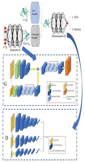
Inspired by the zero-sum game, the training process of the model in the GAN is designed as a confrontation and game between the two networks: the generative network G and the discriminant network D. The schematic diagram of the overall GAN model structure for radar echo extrapolation is as follows (
Figure 1).
In the generative network G, the random noise vector z, obeying the standard normal distribution N(0, 1), is taken as the input, and the generated image G(z) is the output. The generative network tries to generate images that make the discriminative network indistinguishable during training. The generative network G is responsible for the data generation task in the generative adversarial network. For the random distribution of the input samples, the "generated" samples are as similar as possible to the "real" samples. For the generative network G in the GAN network, a new data distribution is generated through complex nonlinear network transformation. In order to make the generated data distribution approach the real data distribution, it is necessary to minimize the difference between the generated data distribution and the real data distribution.
The role of the discriminant network D in the training process is equivalent to that of a binary classification network, which is used to distinguish the actual training image x from the generated image G(z). In this way, the two networks continue to conduct adversarial training, and both are optimized in the process of mutual confrontation. After optimization, the two networks continue to confront each other, and the generated images obtained from the generative network G become closer and closer to the actual images.
Under normal circumstances, the discriminant network assigns the label "1" to the actual image and the label "0" to the generated image. The generative network tries to make the discriminative network "misjudge" the generated image as "1". Suppose
Pr represents the data distribution of the real image
x,
Pg denotes the data distribution of the generated image G(z) and
Pz indicates the prior distribution
N(0, 1) of the random noise vector
z. G and D denote the generation network and the discriminant network, respectively. By using the cross-entropy loss function, the optimization objective of the GAN can be expressed as the following equation (Equation (1)).
where
E is the mathematical expectation. The former term
represents the probability that the discriminant model judges the real original data, and the latter term
represents the probability that the generated data is judged to be false. The GAN optimizes G and D alternately through a Max-Min game until they reach the Nash equilibrium point. Simultaneously, as the alternate optimization proceeds, D will gradually approach the optimal discriminator. When this proximity reaches a certain level, the optimization objective of the GAN is approximately equivalent to minimizing the Jensen–Shannon Divergence between the data distribution of the actual image (
Pr) and the data distribution of the generated image (
Pg). In other words, the principle of the GAN is based on the zero-sum game in game theory, which is equivalent to the optimization of the distribution distance between the actual and generated data.
For the training process of the GAN model only, D is equivalent to a binary classifier. Each update to D enhances its ability to distinguish between the actual and generated images, i.e., correctly assigning two kinds of labels to the two kinds of data and dividing the correct decision boundary between the two kinds of data. The update of G tries to classify generated images as actual images. Thus, the newly generated images are closer to the decision boundary and the actual images. As the alternate iterations continue, the generated images will continue to approach the actual images, eventually making D indistinguishable. Therefore, G can highly and realistically fit the actual data.
3. Temporal and Spatial Generative Adversarial Network (TSGAN)
The GANs are theoretically feasible through mathematical derivation, but they face many problems in the actual training process, the most important of which are gradient disappearance and mode collapse. The reason for the disappearance of the gradient is that the probability of non-negligible overlap between the real distribution and the generated distribution is very small. Therefore, the discriminant network can easily divide the generated data and the real data. The generative network can hardly obtain gradient updates, so it is difficult to optimize the network iteratively. Furthermore, the reason for the mode collapse is that the optimization of the distance between the generated data and the real data distribution is very difficult to control, resulting in the degradation of the generative model and the inability to capture all the changes in the real data distribution.
For the above reasons, inspired by Pix2PixHD [
28], the TSGAN proposed in this study consists of two parts, namely, a dual-scale generator and a multi-scale discriminator. The dual-scale generator uses two radar echo sequences with different resolutions to extract spatiotemporal features. Then, the UNet structure and attention mechanism are used to generate predicted echo sequences. The multi-scale discriminator distinguishes the generated predicted echo sequences at multiple scales. Subsequently, the dual-scale generator is guided to generate higher-quality predicted echo sequences.
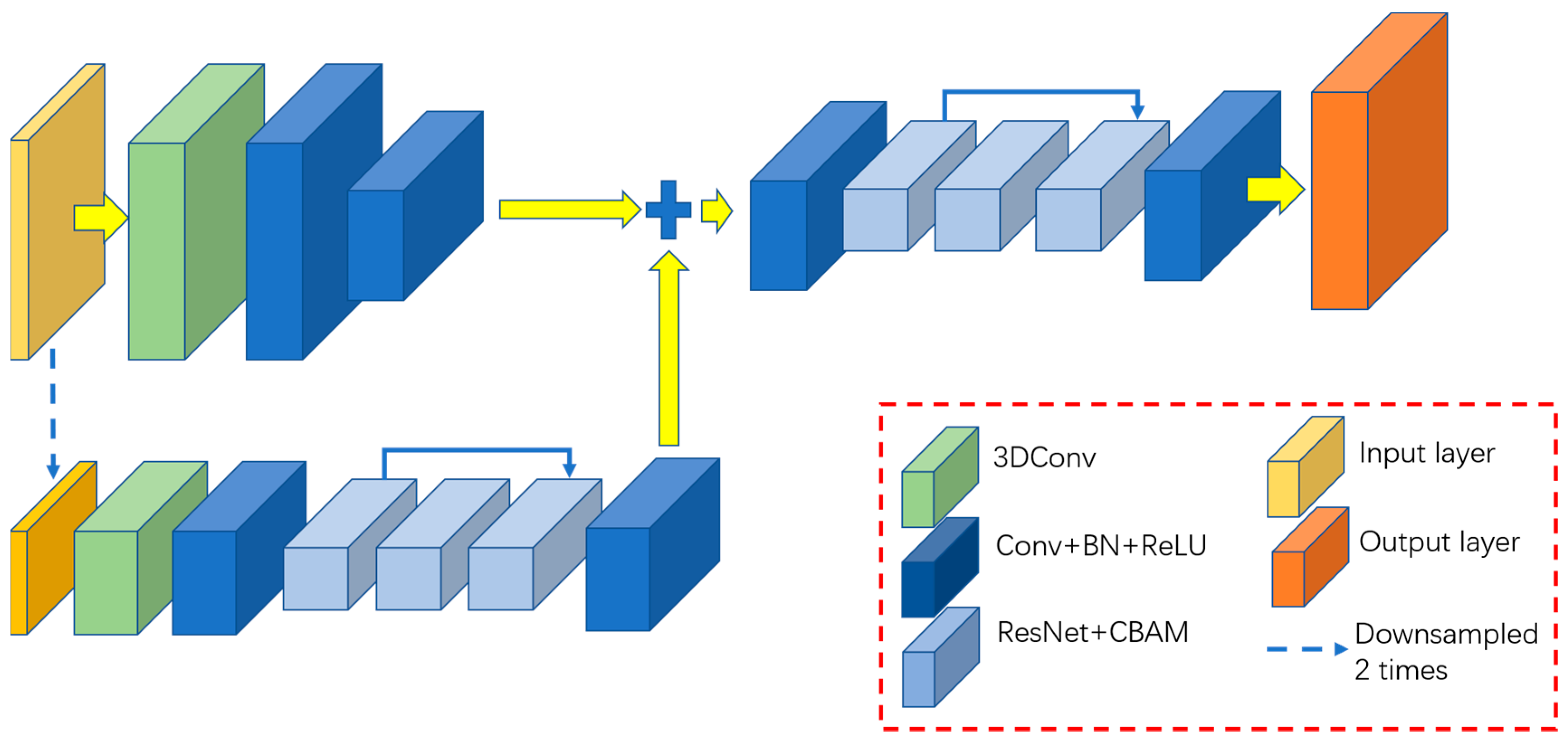
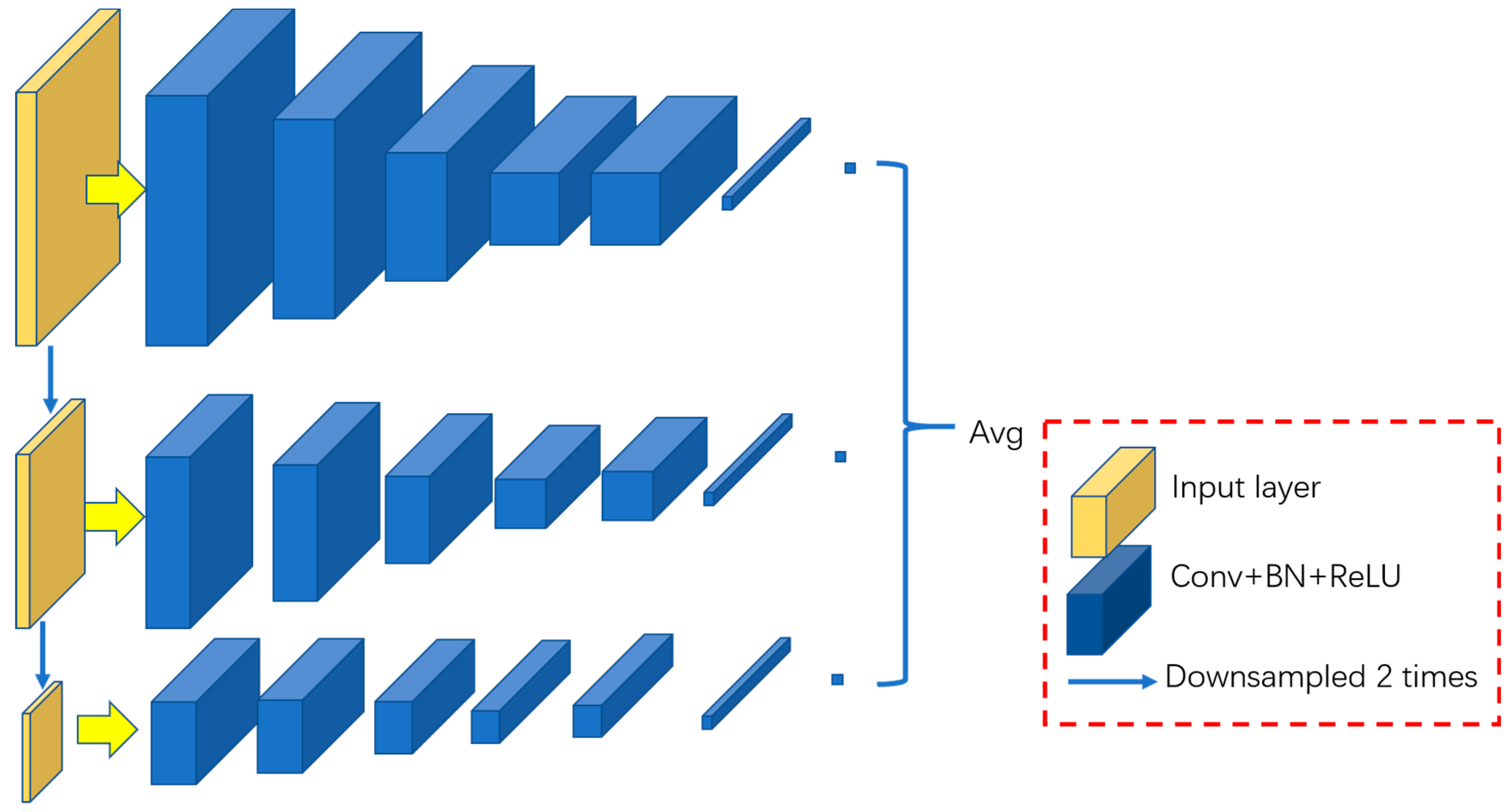
3.1. Dual-Scale Generator
The task of the generator is to use an input radar echo sequence to generate the subsequent 20 frames of the radar echo sequence while retaining as much detailed information of the echoes as possible. Therefore, the spatiotemporal features of the radar echoes need to be considered during this process. A deeper network structure can generate better sequences, but it also faces the problems of overfitting and training difficulties. Therefore, this study is conducted on two scales to take into account the generation effect and network scale. We use three-dimensional convolution to extract the spatial-temporal features of radar echo sequences and employ the UNet structure to restore the spatial details of the generated echo sequences.
The basic structure of the dual-scale generator is shown in
Figure 2:
The input of the generator is the radar echo data of 1 h before the current time. Since the time resolution is 6 min, the input is the radar echo data of 10 consecutive moments, with a size of 896 × 896 × 10 pixels. In terms of the dual-scale generator, the second scale is half of the original scale. At the original scale, the input radar echo sequence (896 × 896 × 10 pixels) passes through several three-dimensional convolutional layers and ordinary convolutional pooling layers to obtain a series of feature maps with a size of 448 × 448 pixels. At the second scale, the input radar echo sequence is down-sampled by a factor of 2, and then the size is changed to 448 × 448 × 10 pixels. The down-sampled data also pass through the three-dimensional convolutional layer and the ordinary convolutional pooling layer. Then, this sequence proceeds through a ResUNet-structured module consisting of the ResNet module [
29] and the CBAM attention mechanism [
30]. The UNet-structured module is composed of modules that resize the output feature maps to the size of the original feature maps, i.e., 448 × 448 pixels. ResUNet replaces the convolution layers in the conventional UNet model with the ResNet module, whose role is to preserve the spatial details of different feature maps as much as possible. The CBAM attention mechanism consists of spatial attention and channel attention, and its role is to preserve the more important information on the space and channel as much as possible. After adding the feature maps of the two scales, the output is restored to the size of the original input radar echoes (896 × 896 pixels) through the convolution pooling layer and the UNet structure module of another ResNet + CBAM layer. Therefore, the final 2 h predicted radar echo sequence is obtained with a size of 896 × 896 × 20.
Two scales are used in the generator. The spatial resolution of the original scale is consistent with that of the input radar echo sequence, which is conducive to retaining the spatial details of the predicted echoes. Because the original scale has the highest spatial resolution, in the process of radar echo time series prediction, almost all of the algorithms will face the problem that the predicted echo becomes more and more blurred as the forecast time increases. The main reason for this is that the spatial detail information is gradually weakened in the process of gradual extrapolation. Using the original scale data, we hope that the spatial details are preserved as much as possible in the network. Meanwhile, the spatial resolution of the second scale is half that of the input radar echo sequence, which facilitates a more thorough control of the orientation of the generator network. The reduction in spatial resolution is equivalent to increasing the receptive field of each convolution kernel, which is beneficial to the network obtaining more global information, thereby controlling the generator network to better fit the trend of future echoes. The balance between the generation effect and the network training can be achieved through the joint action of the spatiotemporal features extracted by three-dimensional convolution and the two scales, obtaining the extrapolation results that not only conform to the development law of radar echoes but also maintain the spatial details.
3.2. Multi-Scale Discriminator
The generated images have high spatial resolution and rich spatial details. Therefore, the discriminator generally needs a deeper network or a larger convolution kernel to ensure that the discriminant network has a larger receptive domain. However, the discriminator may lead to overfitting due to the excessive network capacity and requires more GPU memory for network training.
Therefore, a multi-scale discriminant network is adopted in this study to identify the generated images from different scales, i.e., three discriminators are utilized. The three discriminators all have the same network structure but operate on images of different sizes. Specifically, we down-sample the real and generated images by factors of 2 and 4, respectively, to create image pyramids at three scales. Three discriminators are trained by using different real and generated images of the three sizes. Although the structures of the discriminators are the same, the discriminator with four times down-sampling has the largest receptive field, which ensures that it has more global perspective information and can guide the generator to generate overall consistent images. Additionally, the discriminator at the original scale favors the generator to generate finer details, which also makes the training of the generator easier.
The structure of the discriminant network is shown in
Figure 3, consisting of a series of convolutional layers, pooling layers and fully connected layers. The input size of the original scale discriminator is 896 × 896, and for the second and third scales, it is 448 × 448 and 224 × 224, respectively.
3.3. Loss Function
The loss function consists of three parts, namely, adversarial loss, multi-scale feature loss and overall content loss. Assuming that the discriminator of the network has three scales, “
in” represents the input radar echo sequence, “
tar” represents the future real radar echo sequence, “G” represents the output of the generator network, and
Dk represents the output of the discriminator at the
k-th scale (
k = 1, 2, 3). The total loss function is expressed as Equation (2).
where
and
are the weights of the multi-feature loss
and the overall content loss
. The adversarial loss
in the above formula can be expressed as Equation (3)
The multi-feature loss
can be represented as Equation (4).
where
k (
k = 1, 2, 3) denotes the number of discriminators, and
i represents the
i-th layer of the discriminant network.
The overall content loss
can be obtained according to Equation (5).
where
L1 is the L1 loss, i.e., the MAE loss. The adversarial loss is mainly used to recover the detailed information of the predicted echoes. The multi-scale feature loss and the overall content loss characterize the difference in content between the predicted and observed echoes in the aspects of deep features and pixels. The joint effect of the three loss functions guides the results from the generator to gradually approach the actual radar echoes.
4. Experiments and analysis
The study area is Guangdong Province in southern China. The whole area is located at a latitude of 20°13′ to 25°31′ north and a longitude of 109°39′ to 117°19′. It belongs to the subtropical monsoon climate region. The land spans the northern tropics, the southern subtropics and the central subtropics from south to north. The airflow in this area is particularly strong, and the hot and cold flows frequently meet and collide in this area, resulting in frequent strong convective weather and abundant precipitation. There are many meteorological disasters in the region. The main disasters are: low temperature and rain, strong convection (hail, tornado, strong thunderstorm and strong wind), rainstorm and flood, typhoon, drought, cold dew wind, cold wave, etc. Among them, tropical cyclones and rainstorms have a high frequency and high intensity, ranking first in the country. Meteorological disasters have caused heavy losses to the national economy. For example, Typhoon No. 9615 caused losses of nearly CNY 17 billion to western Guangdong. Therefore, it is extremely important to improve the nowcasting technology.
In this research, the reflectivity factor mosaic data during 2015–2021 from 11 new-generation S-band Doppler radars in Guangdong are used for the experiments. The data in 2015–2019 are selected as the training dataset, the data in 2020 are selected as the validation dataset and the data in 2021 are selected as the test dataset. These original data have horizontal grid points of 700 × 900, with spatiotemporal resolutions of 1 km × 1 km and 6 min. Each sample contains the radar echo input sequence of 10 moments in 1 h and the radar echo target sequence of 20 moments in the next 2 h.
In order to verify the forecast performance of the TSGAN method on extreme convective rainfall, over 80,000 cases in 2021 every 6 min were analyzed. For the page limitation, we only select the squall line process on 4 May 2021 and the typhoon process on 8 October 2021 as study cases for radar echo extrapolation forecasts visualization. Moreover, for comparing the forecasting effectiveness of various methods, the results from the TSGAN method are compared with those from the optical flow [
4], ConvGRU [
19], PredRNN [
21] and PredRNN V2 [
21] methods, which are widely used in the existing operations. The optical flow method employs the Lucas–Kanade algorithm to calculate the optical flow and performs the extrapolation by using the semi-Lagrangian method. The ConvGRU, PredRNN and PredRNN V2 are trained by using the official codes. All of the employed methods should be evaluated by many aspects and multi-dimensions [
31,
32]. By comparing the observed radar echo images, we perform a grid-by-grid test for the prediction accuracy in this study. Additionally, the prediction ability at different radar reflectivity levels is investigated according to the radar reflectivity factors of different intensities. Finally, the critical success index (CSI) is used to evaluate the forecast results quantitatively.
The expression of the CSI is shown in Equation (6).
where
NAk denotes the number of the correct grid points,
NBk denotes the number of false grid points,
NCk denotes the number of missing grid points and k (k = 20 dBz, 30 dBz, 40 dBz and 50 dBz) denotes the threshold value of the different intensities of radar reflectivity. The validation method is adopted according to the forecast leading time and the threshold value. The calculation is performed grid-by-grid, i.e., the predicted and observed values at the same grid point are selected for testing and comparison (
Table 1).
As mentioned earlier, the results obtained by most extrapolation methods suffer from blur, i.e., as the forecast leading time increases, the predicted echoes become more and more blurred, and more details are lost. However, the TSGAN method proposed in this study can recover the detailed information of the radar echoes to a certain extent. To enrich spatial details that are characterized, two indicators, definition and spatial frequency, are introduced in this study. The expression of the definition is as follows (Equation (7)).
The spatial frequency is defined by the frequency in both vertical and horizontal directions. The frequency in the vertical direction is defined as follows (Equation (8)).
The frequency in the horizontal direction is defined as follows (Equation (9)).
Therefore, the overall spatial frequency can be expressed as Equation (10).
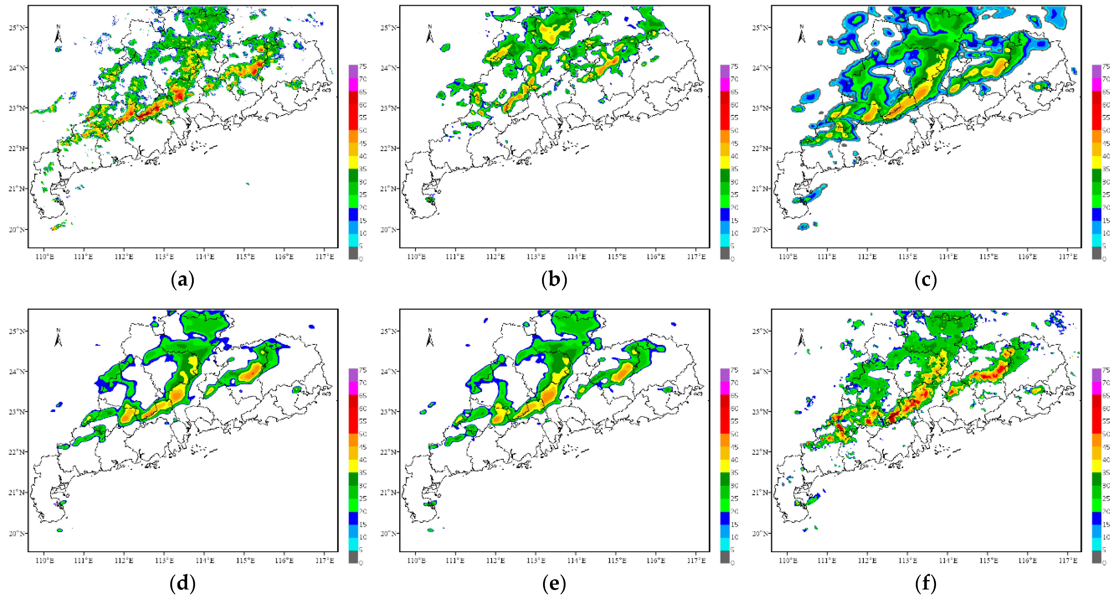
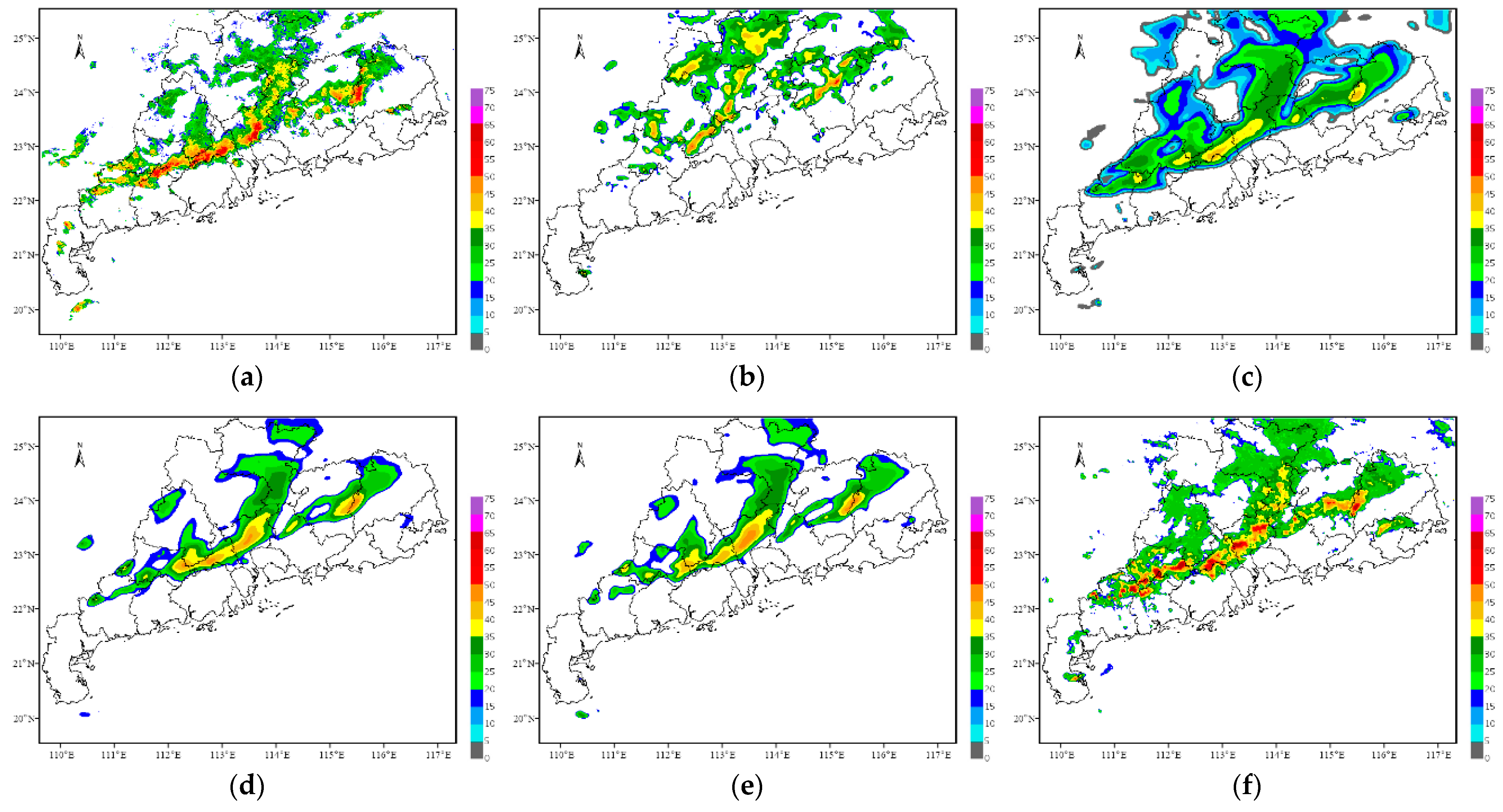
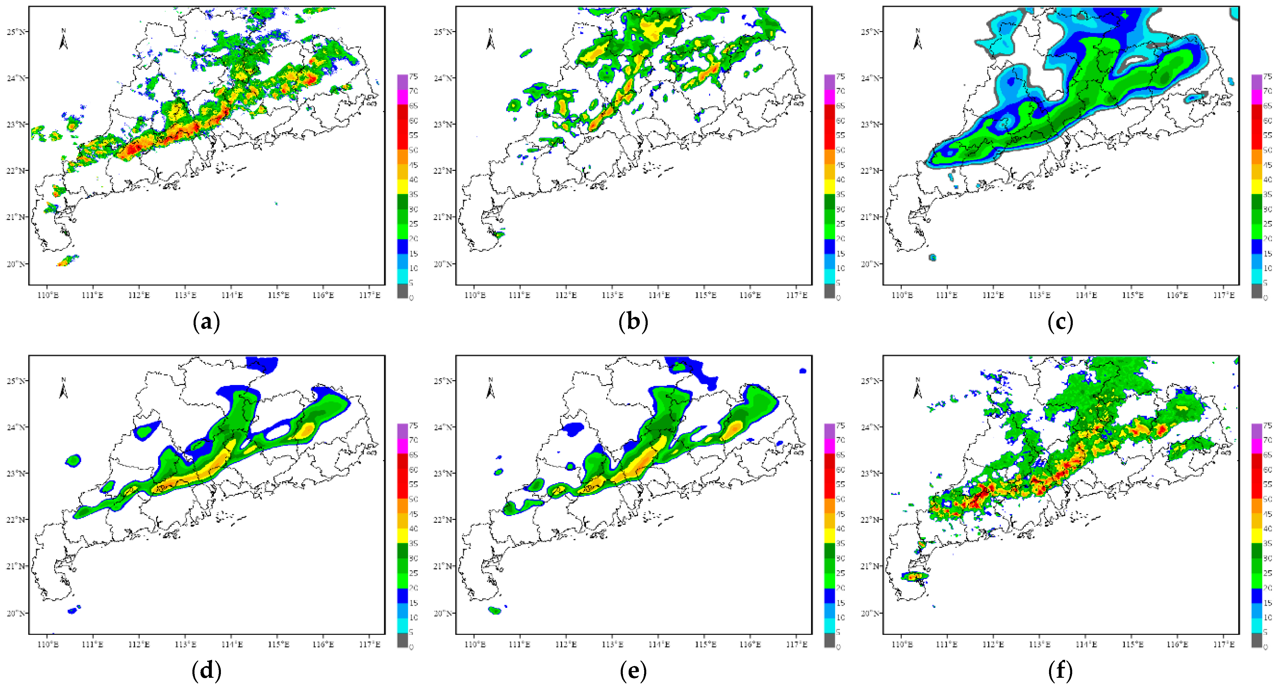
4.1. Squall Line Process on 4 May 2021
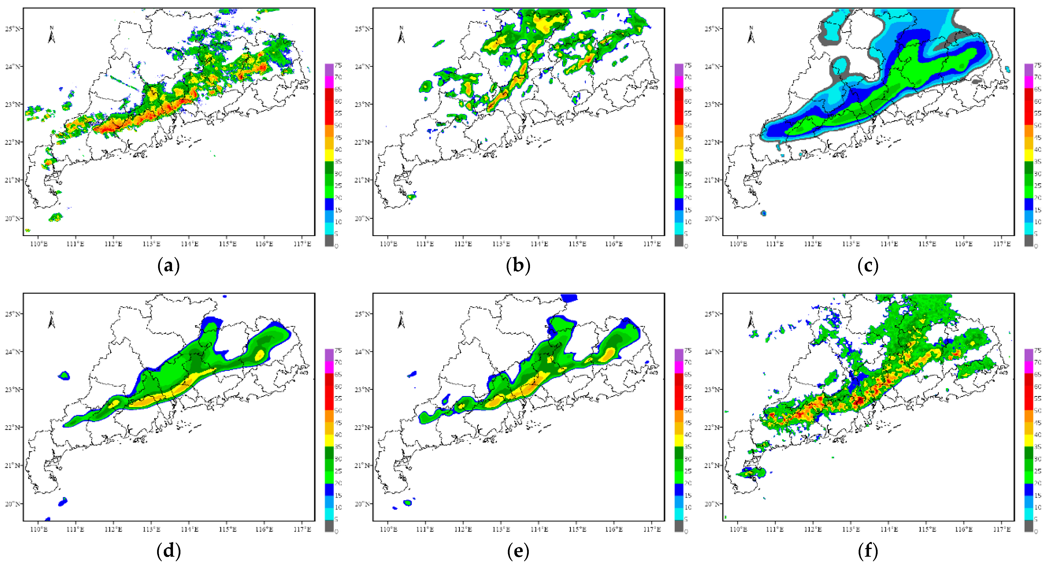
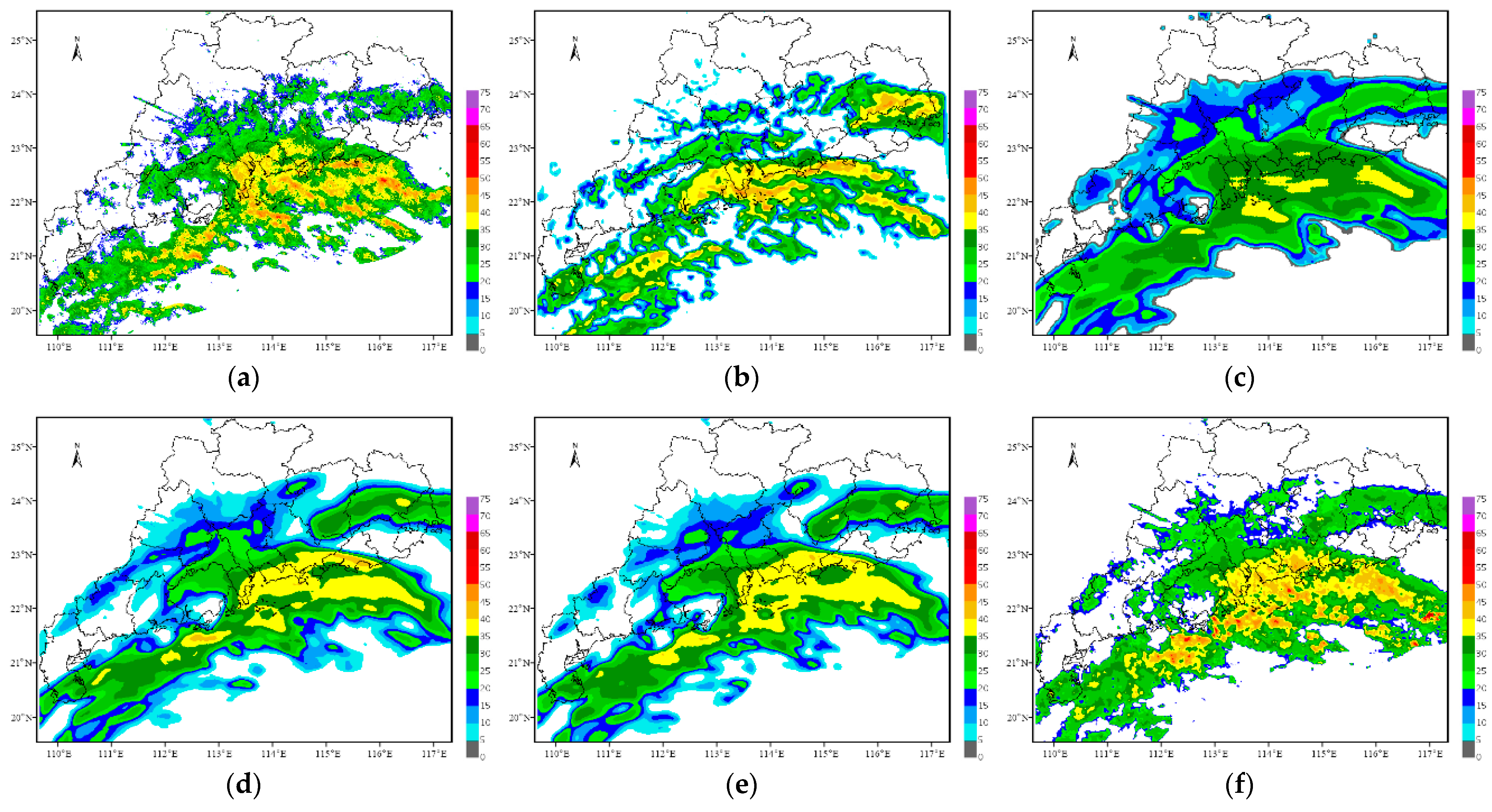
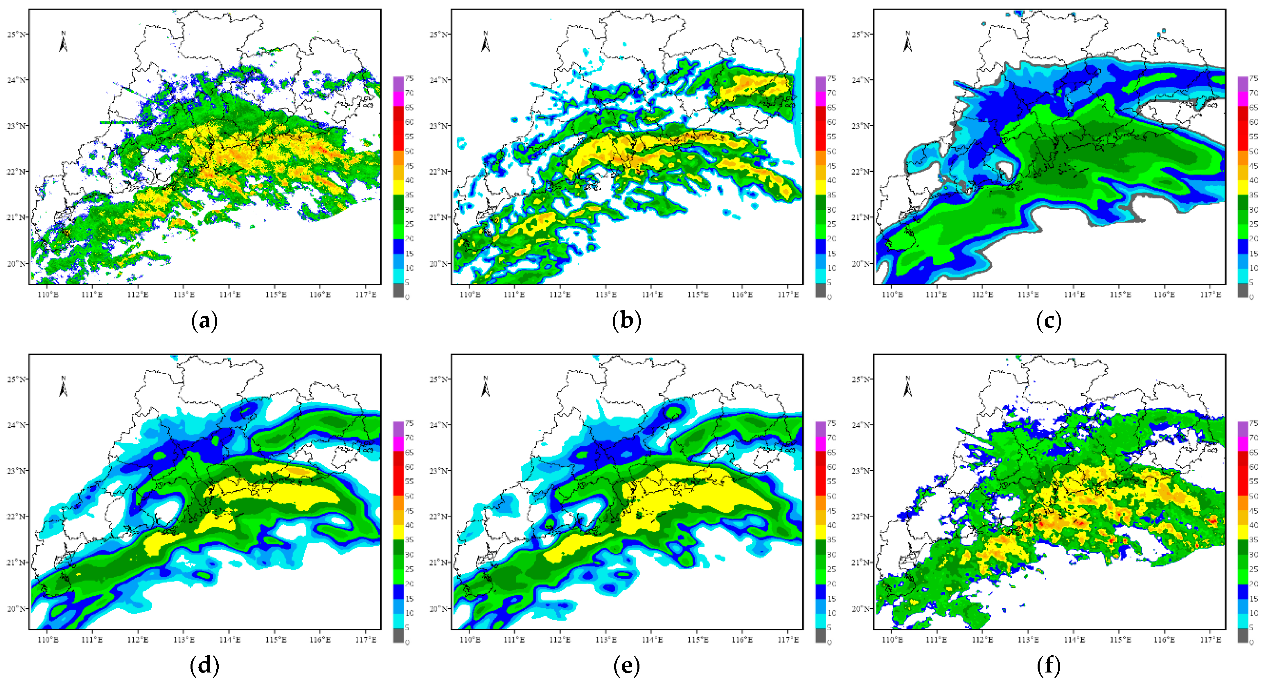
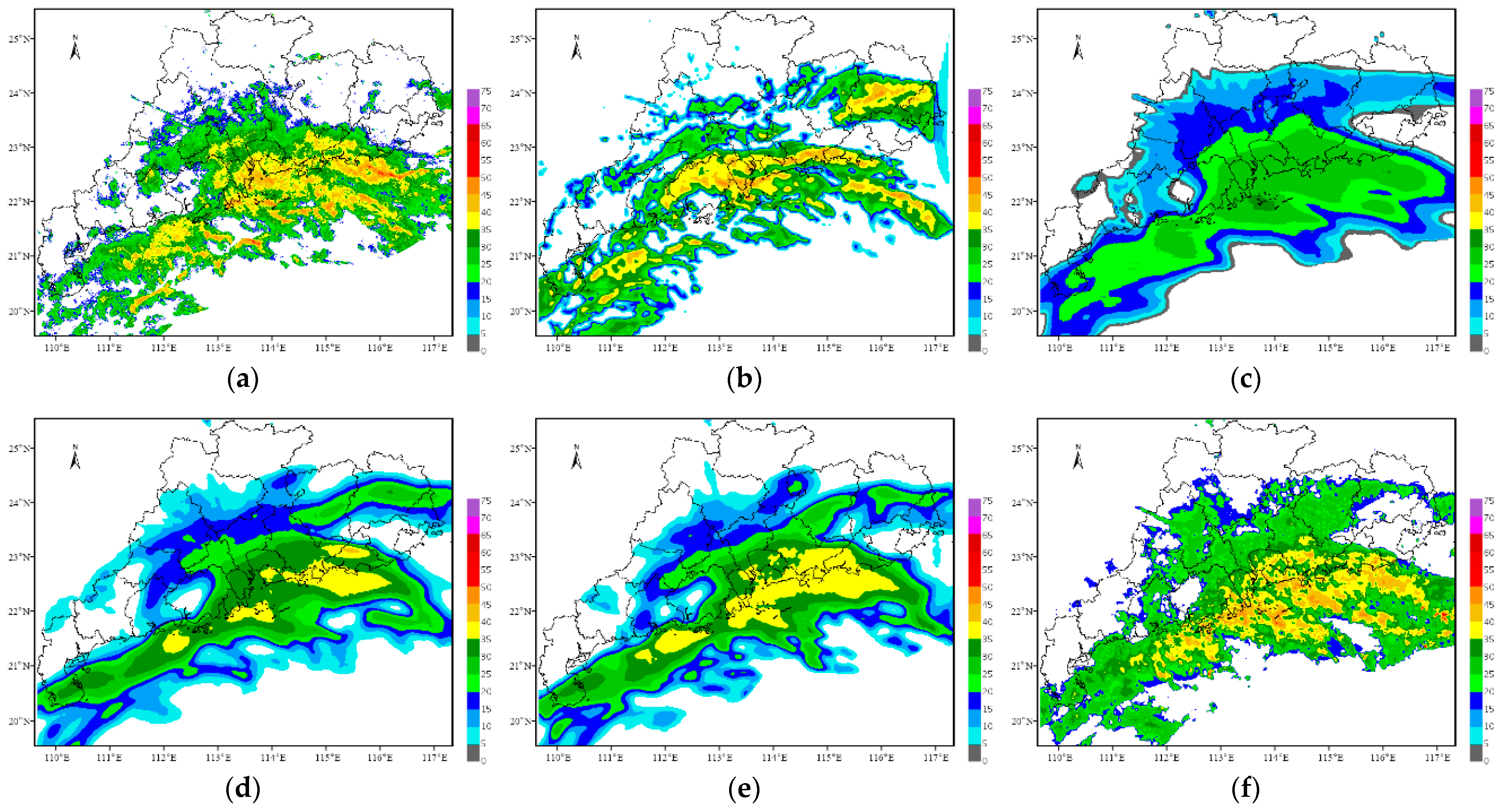
On 4 May 2021, a squall line process swept across Guangdong Province, resulting in extreme heavy rainfall in several areas. In this research, the initial forecast time is 16:00 China Standard Time (CST, same as below) on 4 May 2021, and the echoes for the next 2 h are predicted.
Figure 4,
Figure 5,
Figure 6 and
Figure 7 show the forecast results of this squall line process for the next 0.5 h, 1 h, 1.5 h and 2 h by using each method.
In terms of the overall trend, the difference between the forecast results of the optical flow method and the observations is the largest, where the echo intensity and shape are basically the same, while the difference in the spatial position is the largest among all methods. The other four methods can better grasp the evolution trend of the echoes within 2 h and can also predict the position of the strong echoes. However, except for the TSGAN method, the overall intensity predicted by all the methods decreases rapidly with increasing forecast time. For the detail retained, the forecasts of both the optical flow method and the TSGAN method can present richer detailed information, while those of the other methods become more and more blurred as the forecast time increases. The details predicted by the PredRNN V2 method are slightly better than those predicted by the PredRNN method, and the results of the ConvGRU method are the most blurred. The TSGAN method can retain richer detailed information, and its results do not become more blurred with increasing forecast time.
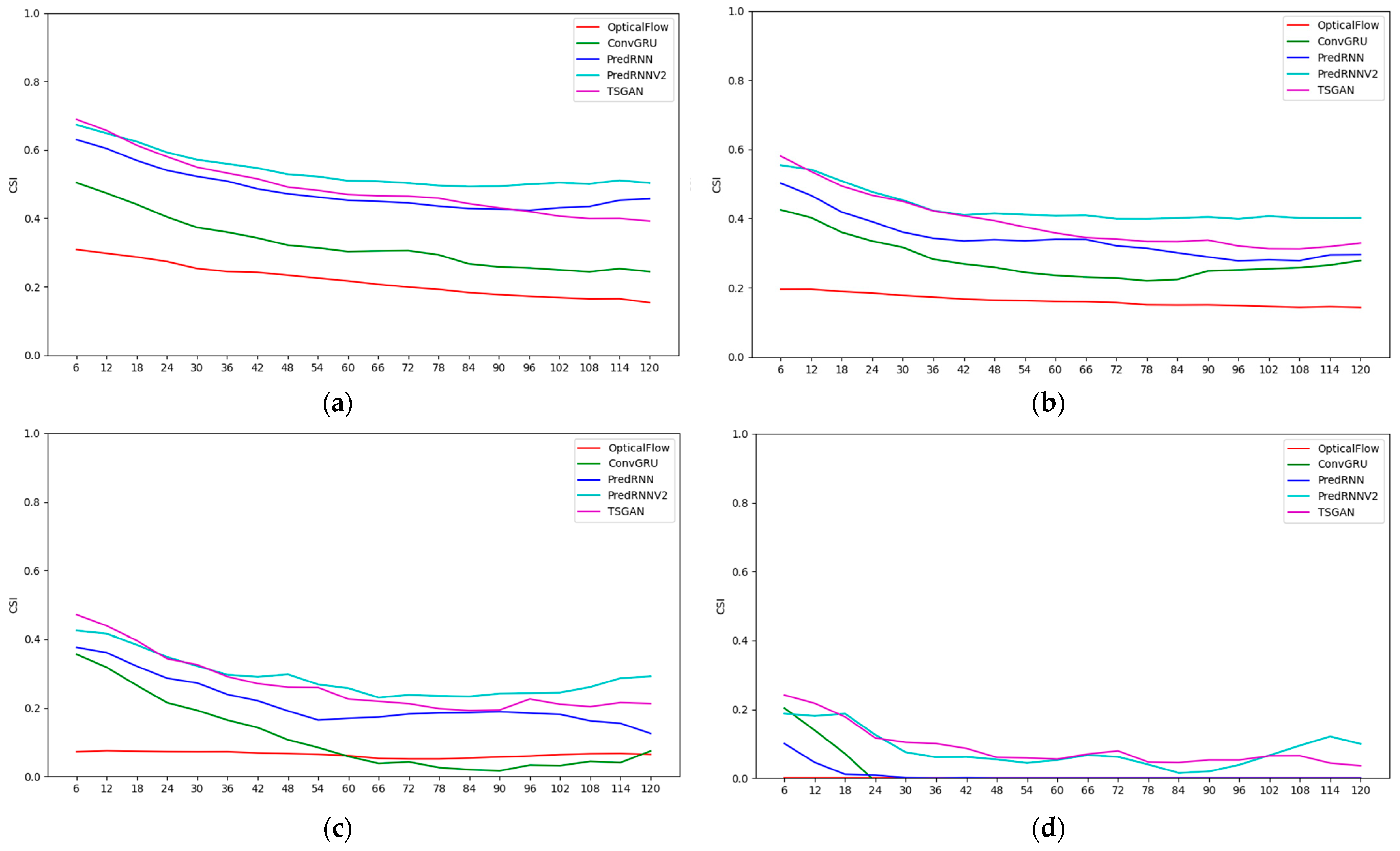
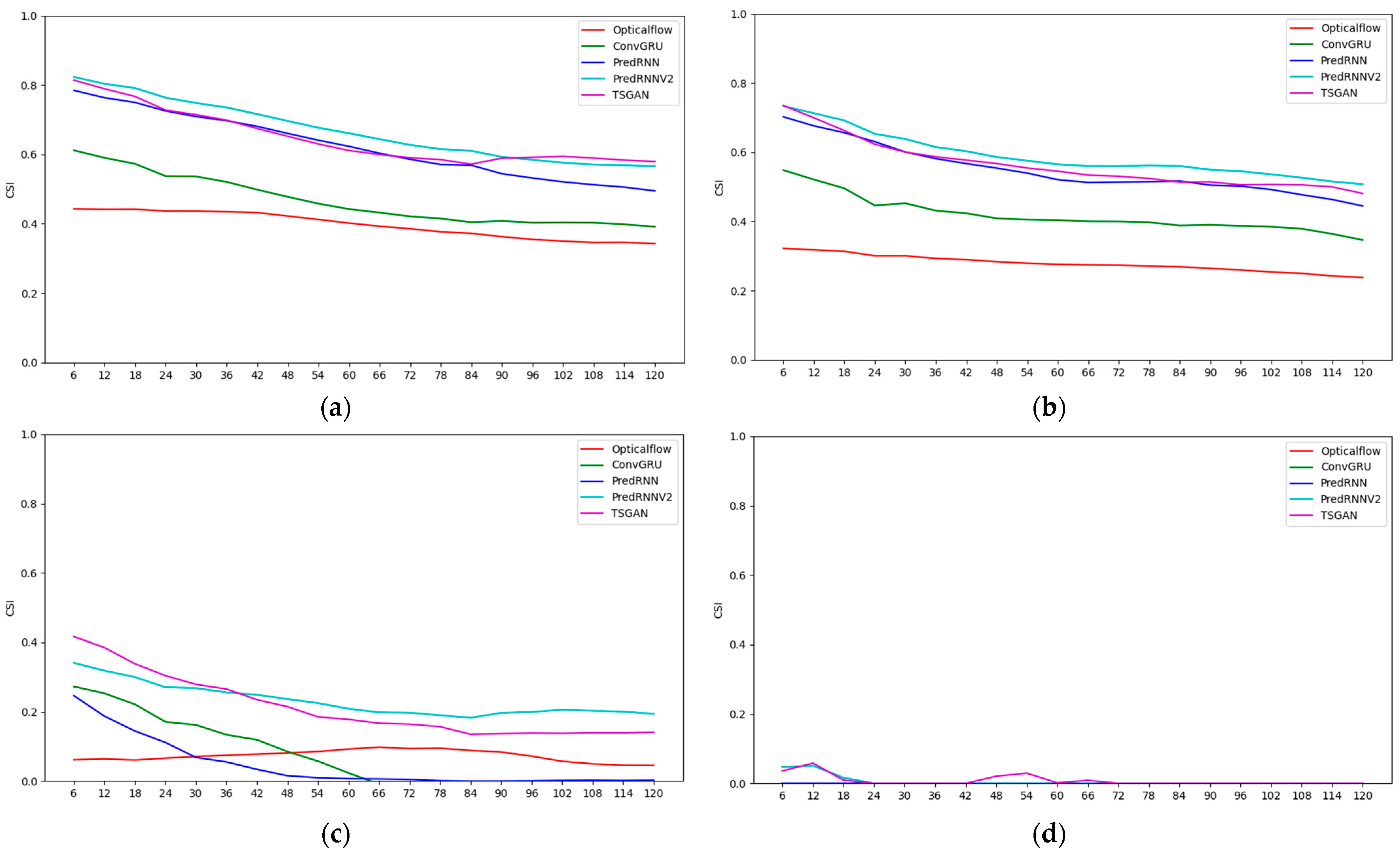
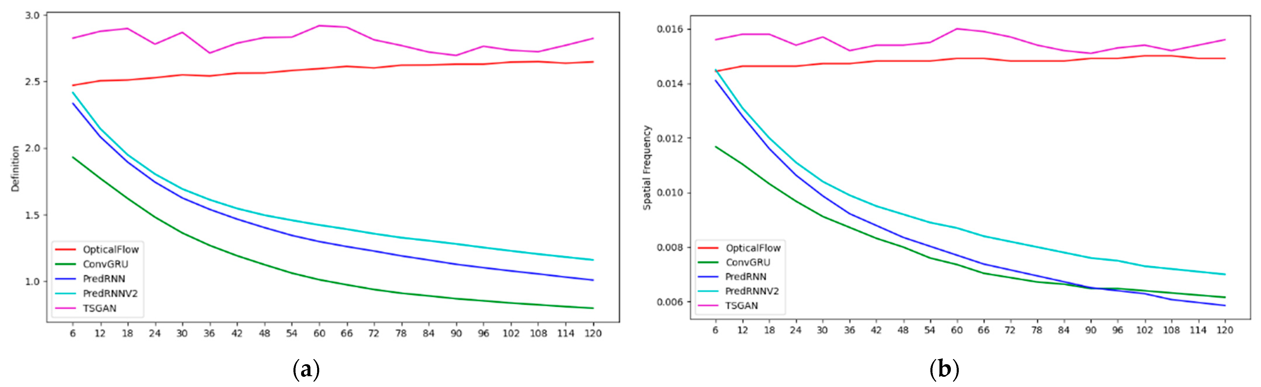
Figure 8 and
Figure 9 present the objective assessment scoring results for each method every 6 min over the 2 h period, and the labels of the horizontal axis are the prediction leading times.
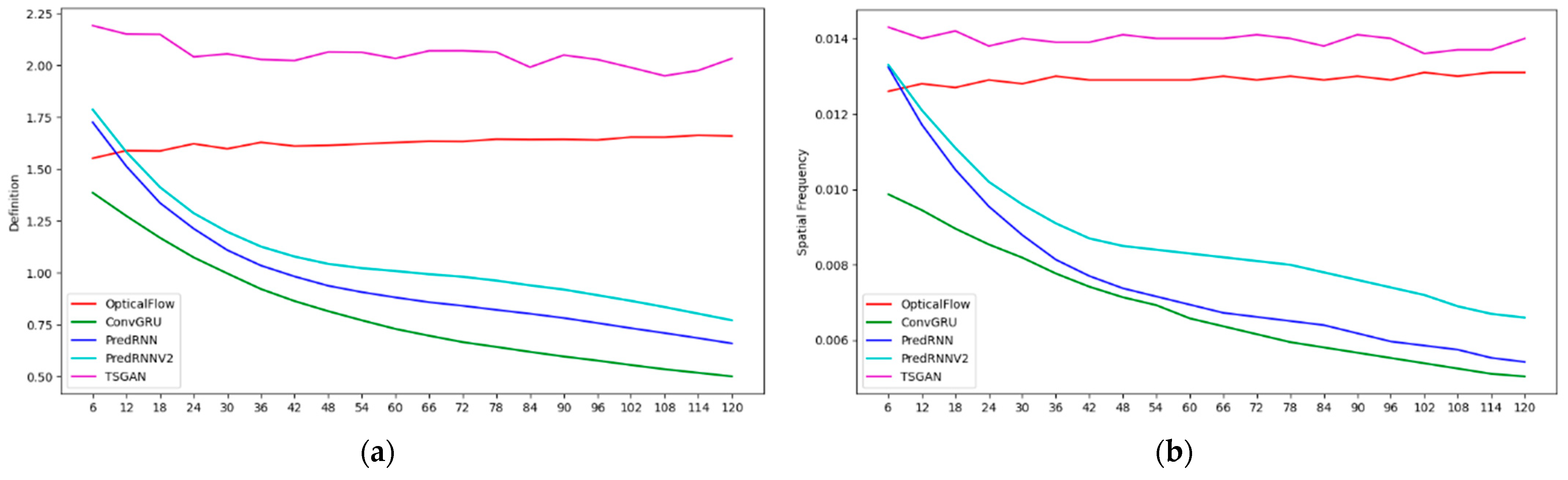
The CSI scores suggest that the CSI values of all methods decrease with the increase in the forecast time, indicating that the longer the forecast time is, the lower the forecast accuracy is. The higher the radar reflectivity is, the more dramatic the CSI value of each method decay is, which means that the longer the forecast time is, the more difficult it is to predict strong echoes. Overall, the PredRNN V2 algorithm performs the best in all reflectivity levels. The PredRNN and TSGAN methods have a little difference between each other, followed by the ConvGRU method, and the optical flow method has the lowest CSI value due to the large deviation in the predicted echo position. In terms of the high-intensity echoes at the 50 dBZ level, the CSI values of the TSGAN and PredRNN V2 differ slightly. The definition and spatial frequency indicators of the ConvGRU, PredRNN and PredRNN V2 methods all show a continuous decreasing trend with increasing forecast time, which is consistent with the fact that their results become more and more blurred. However, for the optical flow method and the TSGAN, the definition and spatial frequency indicators have no obvious decreasing trend, and the definition and spatial frequency values of the TSGAN are higher than those of the optical flow method. This finding indicates that the TSGAN method has obvious advantages in retaining spatial details. Therefore, the comprehensive analysis of the CSI and the spatial information indexes indicates that the TSGAN method performs the best in predicting the squall line process.
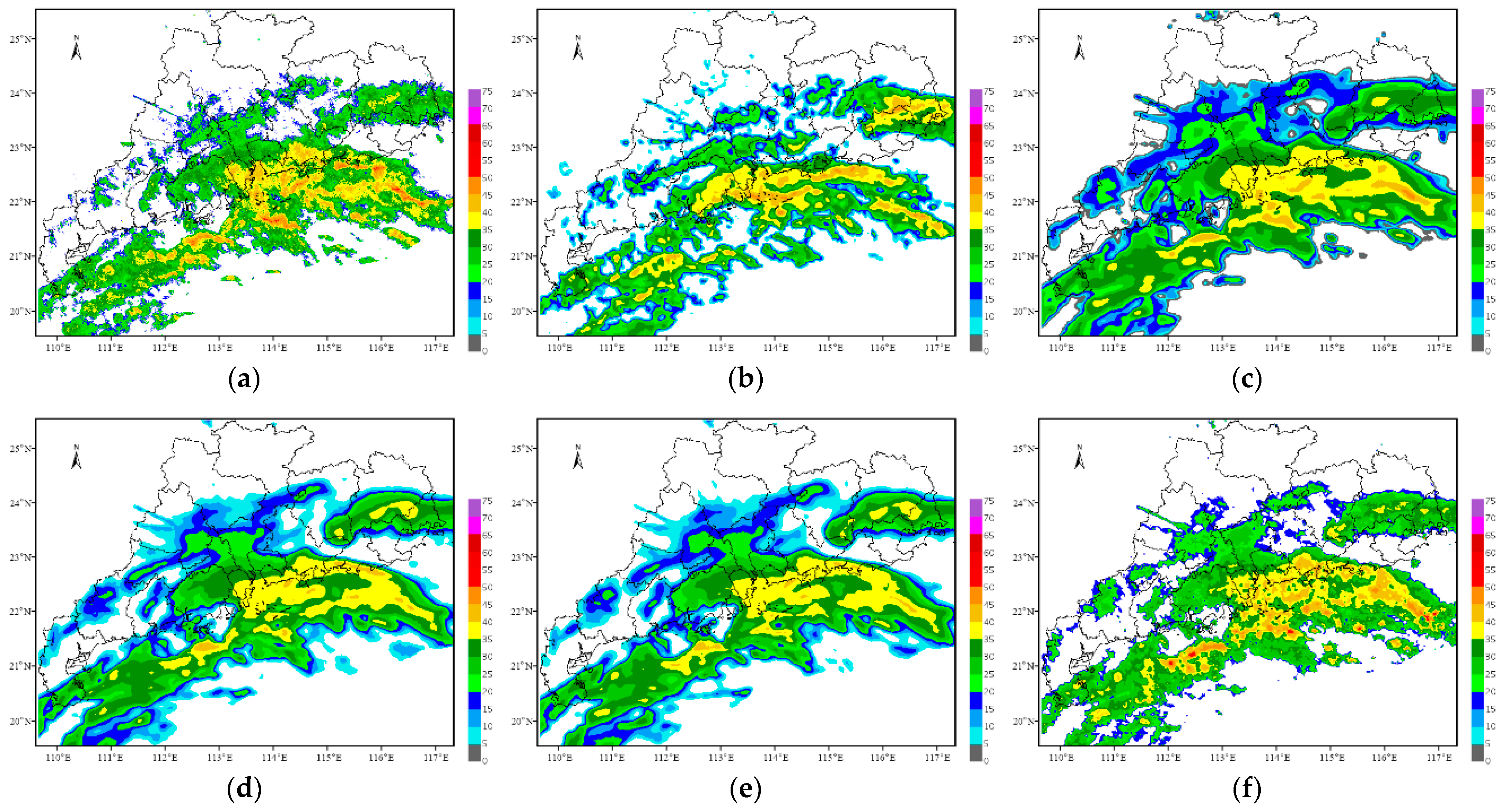
4.2. Typhoon Lion Rock on 8 October 2021
On 8 October 2021, Typhoon Lion Rock was generated, and strong wind and rainfall occurred in the east of Hainan Island and in the south of Guangdong. The precipitation within 6 h in Shenzhen and Shanwei exceeded 80 mm. Furthermore, Shanwei experienced short-term heavy rainfall from 10:00 to 11:00, and the hourly rain intensity reached 34.3 mm. In addition, gusts of 17 m s
−1 and above occurred in Qiongshan of Haikou City and Mulantou of Wenchang City in Hainan Province and in Pinghu of Shenzhen City and Jiuzhou Port of Zhuhai City in Guangdong Province.
Figure 10,
Figure 11,
Figure 12 and
Figure 13 present the forecast results of Typhoon Lion Rock. The initial forecast time is 06:00 on 8 October 2021, and the leading time is 2 h, with an interval of 6 min.
Overall, the forecast results of this typhoon case from each method can better display the development trend of typhoon echoes, and the predicted position is similar to the actual observation. Similar to the previous case on 4 May 2021, the ConvGRU, PredRNN and PredRNN V2 methods still have the problem that as the forecast time increases, the forecast results become more and more blurred, and the predicted radar intensity also weakens considerably. The PredRNN V2 method improves the results of the PredRNN method in detail but still has the problem of blur prediction results. Although the position predicted by the optical flow method changes somewhat within 2 h, the predicted intensity remains basically constant, resulting in strong echoes appearing in the east of Guangdong Province, which is determined by the principle of the optical flow method itself. The forecast results of the TSGAN method retain rich spatial details and are consistent with the observations in intensity and spatial position.
The objective assessment results of the forecasts from each method are presented in
Figure 14 and
Figure 15. The labels of the horizontal axis are the prediction leading times of the future 2 h every 6 min.
The results of the objective assessment indicators have a certain similarity with those of the squall line process. Due to the accurate predicted location and shape of radar echoes, the PredRNN V2, TSGAN and PredRNN methods show apparent advantages in the CSI scores. The spatial location of the optical flow method is not satisfactory in terms of accuracy. Thus, the CSI scores of the optical flow method are lower than those of the ConvGRU method. The PredRNN V2 method has a noticeable improvement in detail compared with the PredRNN method but still suffers from blur. In terms of definition and spatial frequency indicators, similar to the case on 4 May 2021, the TSGAN and optical flow methods can maintain stable spatial detail forecasts in each forecast time, while the other three methods become more and more blurred with increasing forecast time, resulting in more detail loss. In summary, the objective assessment suggests that the TSGAN method has certain advantages in forecasting this typhoon process while retaining more spatial details.


 ,
, 


