Article

ENSO Impact on Winter Precipitation in the Southeast United States through a Synoptic Climate Approach

1
Savannah River National Laboratory, Aiken, SC 29808, USA
2
Lamont-Doherty Earth Observatory, Columbia University, Palisades, NY 10960, USA
*
Author to whom correspondence should be addressed.
Atmosphere 2022, 13(8), 1159; https://doi.org/10.3390/atmos13081159
Submission received: 1 June 2022 / Revised: 19 July 2022 / Accepted: 21 July 2022 / Published: 22 July 2022

Abstract

:
The ENSO impact on winter precipitation in the Southeast United States was analyzed from the perspective of daily weather types (WTs). We calculated the dynamic contribution associated with the change in frequency of the WTs and the thermodynamic contribution due to changes in the spatial patterns of the environmental fields of the WTs. Six WTs were obtained using a k-means clustering analysis of 850 hPa winds in reanalysis data from November to February of 1948–2022. All the WTs can only persist for a few days. The most frequent winter weather type is WT1 (shallow trough in Eastern U.S.), which can persist or likely transfer to WT4 (Mississippi River Valley ridge). WT1 becomes less frequent in El Niño years, while the frequency of WT4 does not change much. WTs 2–6 correspond to a loop of eastward propagating waves with troughs and ridges in the mid-latitude westerlies. Three WTs with a deep trough in the Southeast U.S., which are WT2 (east coast trough), WT3 (off east coast trough) and WT6 (plains trough), become more frequent in El Niño years. The more frequent deep troughs (WTs 2, 3 and 6) and less frequent shallow trough (WT1) result in above-normal precipitation in the coastal Southeast U.S. in the winter of El Niño years. WT5 (off coast Carolina High), with maximum precipitation extending from Mississippi Valley to the Great Lakes, becomes less frequent in El Niño years, which corresponds to the below-normal precipitation from the Great Lakes to Upper Mississippi and Ohio River Valley in El Niño years, and vice versa in La Niña years. The relative contribution of the thermodynamic and dynamic contribution is location dependent. On the east coast, the two contributions are similar in magnitude.

1. Introduction

The influence of the El Niño–Southern Oscillation (ENSO) on the U.S. climate is strongest during the winter [1,2]. The problem is usually studied based on seasonal means, such as the ENSO impact on the mean precipitation in December–February [3]. As we experience in everyday life, climate and its variability are actually manifested by daily weather. Therefore, it is equally important to learn how the ENSO impacts daily weather. The problem will be examined and quantified using a weather typing (WT) analysis in the Southeast United States (SEUS) for the winter in the current study. A Similar method was applied in a study on the impact of the ENSO in other places in the world, such as in the Northeast U.S. [2,4] and in Southeast Asia [5,6,7,8], as well as on spring precipitation in the SEUS [9]. The rationale for the WT analysis and reference therein can be found in Qian el al. [9].
From the large-scale point of view, winter WTs in the SEUS are closely related to the North Atlantic Subtropical High (NASH) south of the Gulf coast (along about 30° N) and westerly winds north of 30° N, as shown in the monthly climatology in Figure 1. However, the monthly precipitation and 850 hPa circulation of the four months from November to February look almost the same, especially in the deep winter months of December to February, with the anticyclonic circulation of the NASH withdrawn further to the south. Winter rainfall is often produced by southwesterly flows ahead of a cold front that brings moisture from the warmer Gulf of Mexico. The location of precipitation should depend on the weather regime of the day, especially the longitude of the trough. However, the ridges and troughs cannot be seen from the monthly or seasonal mean figures. As will be seen shortly, the weather typing analysis brings up the dynamic view of these propagating ridges and troughs. Cold air damming east of the Appalachian Mountains can also bring cold weather to the south in the winter [10,11]. Geographically special for the east coast, the strong temperature gradient between the warm Gulf Stream off the east coast and the cold coastal land in the cold seasons also forms a baroclinic belt, which corresponds to the quasi-stational east coast trough and storm track, as seen from the heavy precipitation along the east coast in Figure 1. All these are important factors that affect winter weather in the SEUS.
In the following, we will first describe the data and method briefly, then examine the spatial pattern and frequency of the winds and precipitation of the WTs. Finally, we will use the characteristics of the WTs to interpret the ENSO impact on precipitation in the SEUS.

2. Data and Weather Typing Analysis

2.1. Data

As in Qian et al. [7,9], the 850 hPa wind components of the NCEP-NCAR Reanalysis Project-I (NRP) data [12], from 1 January 1948 to 28 February 2022, are used for the WT analysis. To examine the precipitation pattern of each of the WTs, the satellite estimated 3-hourly precipitation data from CMORPH (NOAA Climate Prediction Center-CPC Morphing Technique, 0.25° × 0.25°, 1998–2020, covering both land and sea) [13] were used to plot the precipitation maps. The CPC-unified gauge-based analysis of daily precipitation over the contiguous United States (CONUS) at quarter-degree grids in 1948–2022 (https://psl.noaa.gov/data/gridded/data.unified.daily.conus.html, accessed on 20 July 2022, covering only land area) is used for analyzing the ENSO impact on precipitation.

2.2. WT Analysis

The domain used for the WT analysis, 100–65° W and 20–45° N, is the same as was used to analyze the WTs in the warm season in the SEUS [9]. In this paper, we analyze November to February. We also extend the years of analysis by including all currently available NRP data: 1948–2022.
As in Roller et al. [2] and Qian et al. [7,9], the classifiability index (CI) is calculated to determine the optimum number of clusters for the dataset, with large CI indicating a better separation between clusters. The optimum number of clusters (k) corresponds to the peak in CI following the initial decrease. The daily weather in the SEUS in the winter can be best represented by six clusters (k = 6) (Figure 2).

3. Results

3.1. Winter Weather Types in the SEUS

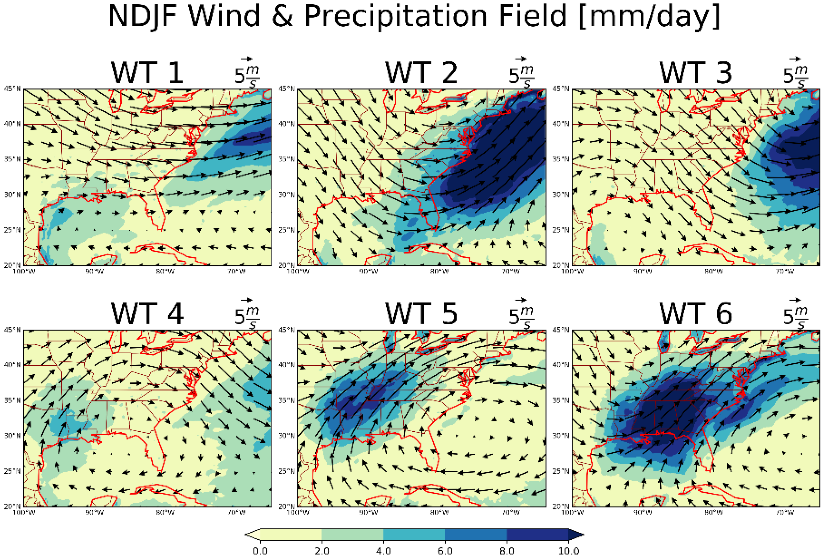
The spatial distribution of the 850 hPa winds for the six WTs, along with the associated mean precipitation of each, is shown in Figure 3 and a brief description is given in Table 1. WT1 represents a broad and shallow trough over central-east US. WT2 is an east-coast trough with precipitation ahead of the trough along the east coast from Florida to the mid-Atlantic coast, but with maximum precipitation over the costal ocean along the Gulf Stream. Behind the trough, northwesterly dry flow takes place over the Midwest and Great Plains. The Gulf coast is also quite dry. WT3 is an off-east-coast trough with maximum precipitation over the ocean, while the land in the Central and Eastern U.S. is dry. WT4 features a ridge over the Mississippi River Valley, with a trough and rainy area in the Atlantic Ocean quite far away from the east coast. The east coast and the Great Lakes area are dry. The southern Great Plains get some rainfall with moisture supplied by the southerly flow from the Gulf coast. In WT5, a trough is over the western Great Plains, with the southwesterly flow bringing forth moisture and precipitation over the Mississippi River Valley. An anticyclone is centered off the east coast of the Carolinas. The east coast is quite dry. In WT6, a deep trough is over the eastern Great Plains and the Mississippi and Missouri river valleys. The strong southwesterly flow east of the trough transports moisture from the Gulf of Mexico and dumps heavy precipitation in the Mississippi River Valley and SEUS.
Comparing the winter WTs to those WTs in March–October, given in [9], some WTs are similar to or even identical to each other. For instance, the WT2 in Figure 3 here is quite similar to the WT1 (ECT) in [9]. WT4 here in Figure 3 is almost identical to the WT2 (MRVR) in Qian et al. [9], while WT6 here in Figure 3 is similar to the WT3 (PT) in Qian et al. [9]. It is reasonable that some WTs in November–February may share similar features of the WTs in the transitioning seasons of spring and fall, contained in the period of March–October in Qian et al. [9].
WT5 bears some similarity to the WT6 (Figure 3), but with a shallower trough in the western Great Plains. WT5 is also somewhat similar to the warm season WT6 (Carolina High, [9]), but the anticyclone center in the WT5 here is off the Carolina coast, while the warm season WT6 has the Carolina High centered on the coast.
We cannot find similar warm season WTs similar to the winter WT1 and WT3; therefore, they are distinctively winter WTs. In the winter, with the contrast of cold continent and warm ocean, the general circulation favors a quasi-stationary trough along the east coast of the continents. This is manifested by the occurrence of a shallow trough in coastal land (WT1) and a deep off-shore trough (WT3).
It is also worth noting that precipitation is heavy over the Great Lakes (near the northern border of the domain in Figure 3), as compared to the surrounding lake shore region, in WTs 5 and 6, in which southwesterly flow brings moisture toward the Great Lake region. In the winter, surface temperature over the lakes should be warmer than that over the land. Therefore, moist air and the warm lake surface both work to increase the conditional instability of the atmosphere, thus, enhancing precipitation over the lakes.

3.2. Frequency of the WTs

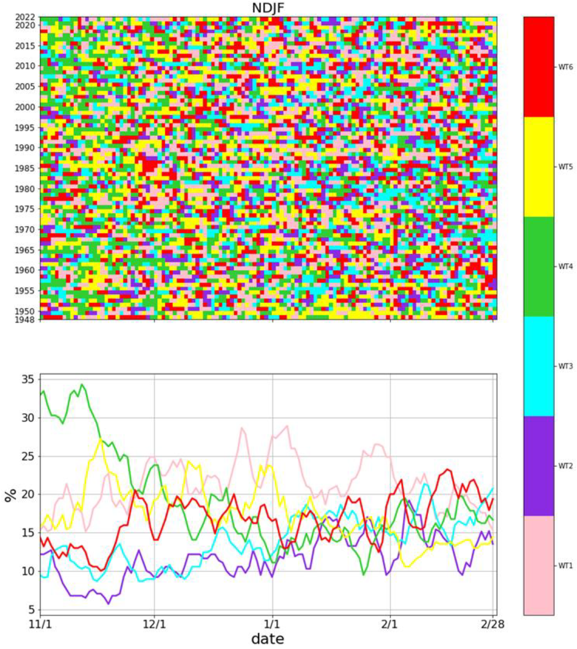
From 1 November to 28 February of 1948–2022 (120 days per year for 74 years, 8880 days in total), the percentages for the total number of days with WT 1–6 are 21.3%, 11.7%, 13.9%, 19.0%, 17.5% and 16.7%, respectively. The occurrence of the daily WTs through the season is shown in Figure 4. All six WTs sporadically occur in the winter season, as can be seen from the top panel in Figure 4. WT1, a distinctive winter WT, occurs quite frequently in every month of the winter, especially in December and January; therefore, it is the most frequent WT in the center of the winter. In the winter, westerly winds are the strongest in the mid-latitude due to the strongest baroclinicity (Figure 1), which corresponds to the quite zonal flow of WT1. WT2 (ECT), the least frequent winter WT, occurs slightly more in January and early February. As mentioned before, the WT2 (ECT) here is similar to the WT1 (also ECT) in [9] that frequently occurs in March–April. Therefore, ECT is common in the winter and spring in the SEUS. WT3 (OECT), the second least frequent winter WT, occurs more in January and February. WT4 (MRVR, the second most frequent WT) occurs more frequently in November (especially in the early part of the month) and least frequently in January. A precipitation map of WT4 indicates that it corresponds to fair weather in most of the SEUS, except for the southwest portion of the region. In other words, the fair weather in late fall in the SEUS is due to frequent WT4 (MRVR). WT5 (WPT) is more frequent in the first half of the winter (from mid-November to early January) with a contrast of rainy weather west of the Appalachian and fair weather along the east coast. Finally, WT6 is less frequent before late November and then somewhat evenly distributed after that. Comparing to the warm season WTs with a dominant summer WT (Florida High Zone that occurs about 60% of days in July, see [9]), there is no single dominant WT in the winter.
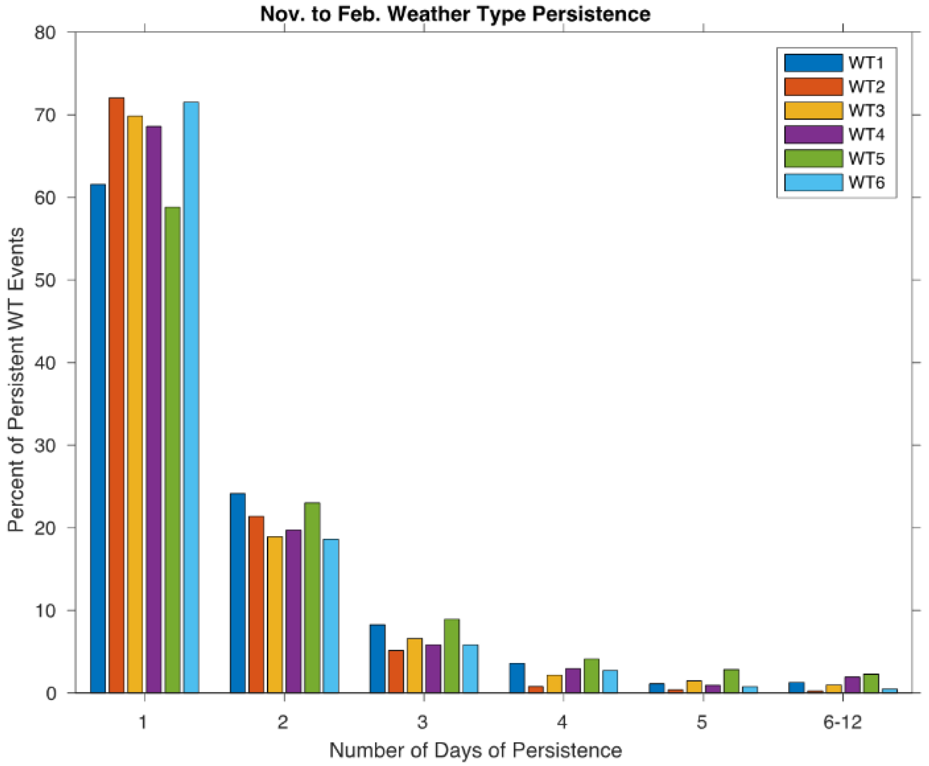
Figure 5 shows the persistence of the WTs. For all six WTs, over 50% of their respective occurrences persist for only one day (and progress to other WTs the next day) and 20% persist for 2 days, 5–10% persist for 3 days and very few can persist for 4–12 days. These are short compared to the summer WTs that can persist for up to 20 days [9]. Winter weather is mostly controlled by eastward propagating baroclinic waves and, therefore, they have short persistence and fast transition/progression from one WT to another.
The progression of the WTs is shown in Figure 6. WT1 significantly progresses to itself (i.e., persistence, due to its nearly zonal flow) and also likely progresses to WT4 (shown by red bars). Actually, persistence is statistically significant for every WT (red bar). Besides persistence, the preferred progression loop is from WT2 (ECT) to WT3 (OECT), to WT4 (MRVR), to WT5 (WPT), to WT6 (PT) and then back to WT2. The circulation patterns of WTs 2–6 (Figure 3) indicate that the above progression loop corresponds to the eastward propagation of westerly waves.
We also checked the long-term trend in the 1948–2022 time series for the frequency of each of the WTs in November to February (figure not shown) and did not find a significant trend based on the Mann–Kendall test at the 95% significance level.

3.3. ENSO Impacts on Rainfall in the SEUS in the Winter

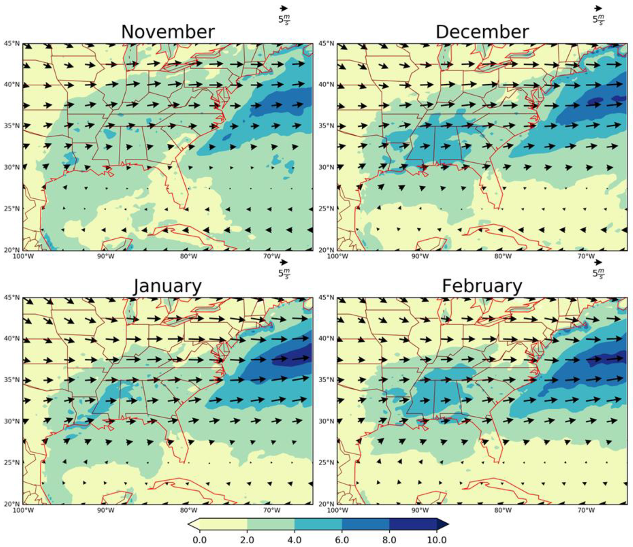
After analyzing the frequency and spatial pattern of the WTs, we can then use them to interpret the ENSO impact on the winter precipitation in the SEUS. As can be seen from Figure 1, the monthly climatology is similar among each month in deep winter months of December to February (DJF); therefore, we will focus on DJF.
As conducted by Ohba and Sugimoto in [14] for the ENSO impact on precipitation in Japan, we also quantified the dynamic and thermodynamic contributions of ENSO to the winter precipitation in the SEUS. El Niño and La Niña have the opposite impact, but may not be totally asymmetric, so we will check their impact separately. The anomalous precipitation associated with El Niño (denoted by En) can the written as:
δ P = P E n P C l i m = i = 1 K p i E n f i E n i = 1 K p i C l i m f i C l i m = δ P thermo + δ P d y n
K = 6 is the number of the WTs; P E n and P C l i m are the precipitation in El Niño years and the climatology (all year average), respectively; p i E n and p i C l i m are the precipitation of WT i (i = 1 to 6) in El Niño years and climatology, respectively; f i E n and f i C l i m are the frequency of WT i in El Niño years and climatology, respectively; and δ P t h e r m o and δ P d y n are the thermodynamic and dynamic contribution to the anomalous precipitation, respectively, as follows:
δ P t h e r m o = i = 1 K ( p i E n p i C l i m ) f i E n + f i C l i m 2
δ P d y n = i = 1 K p i E n + p i C l i m 2   ( f i E n f i C l i m )
The δ P t h e r m o in (2) is resulted from the changes in the basic (environmental) field, such as temperature and moisture. The δ P d y n in (3) is caused by the changes in frequency of the WTs. The thermodynamic and dynamic contribution to precipitation anomalies in La Niña (denoted by Ln) can be calculated similarly, by replacing En by Ln in (1) to (3).
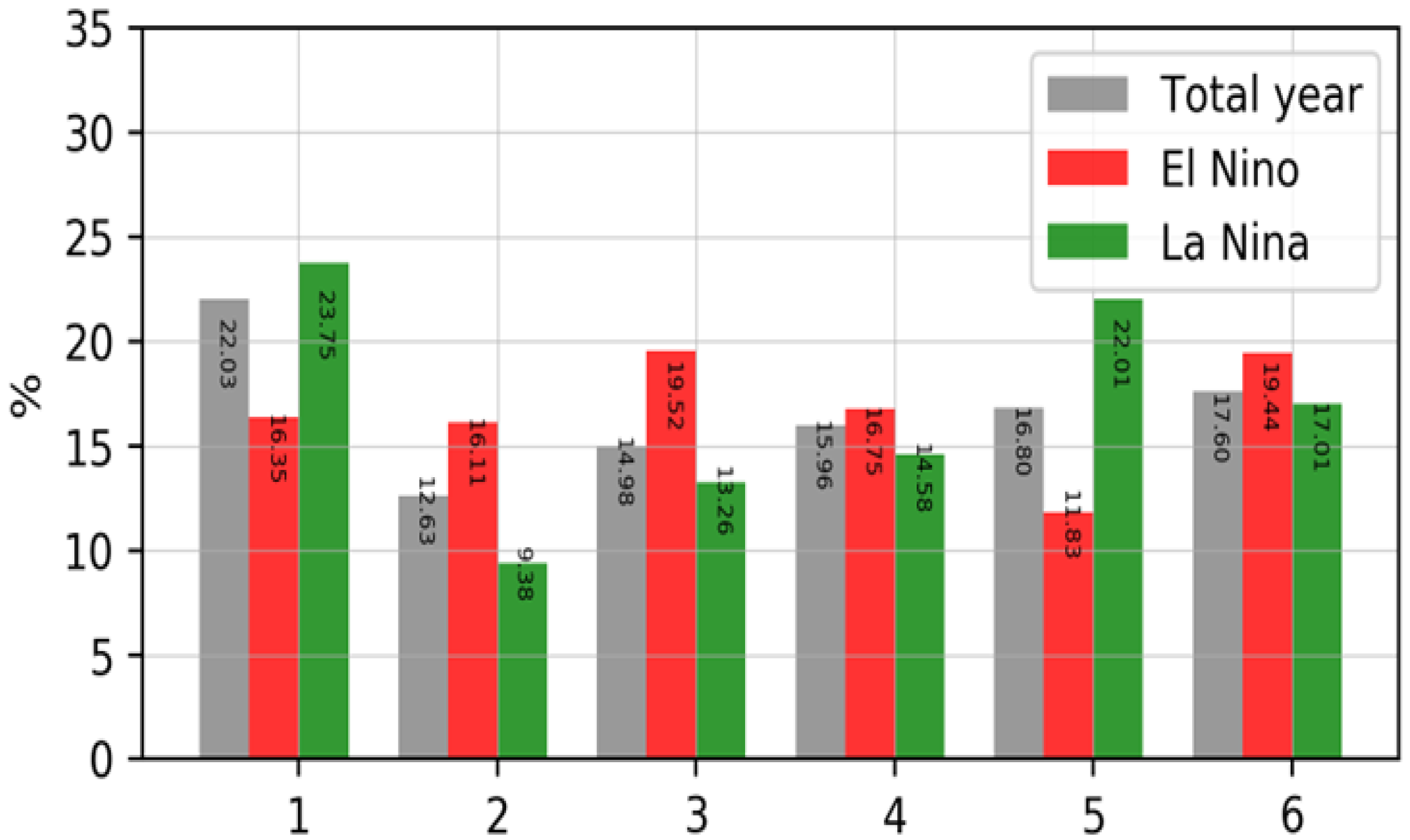
Figure 7 shows the frequencies of the winter WTs in El Niño, La Niña and all years in DJF ( f i C l i m , f i E n   and   f i L n ,   i = 1 ,   6 ) . In El Niño years, the frequencies of WTs 1 and 5 decrease, those of WTs 2, 3 and 6 increase and that of WT4 slightly increases.
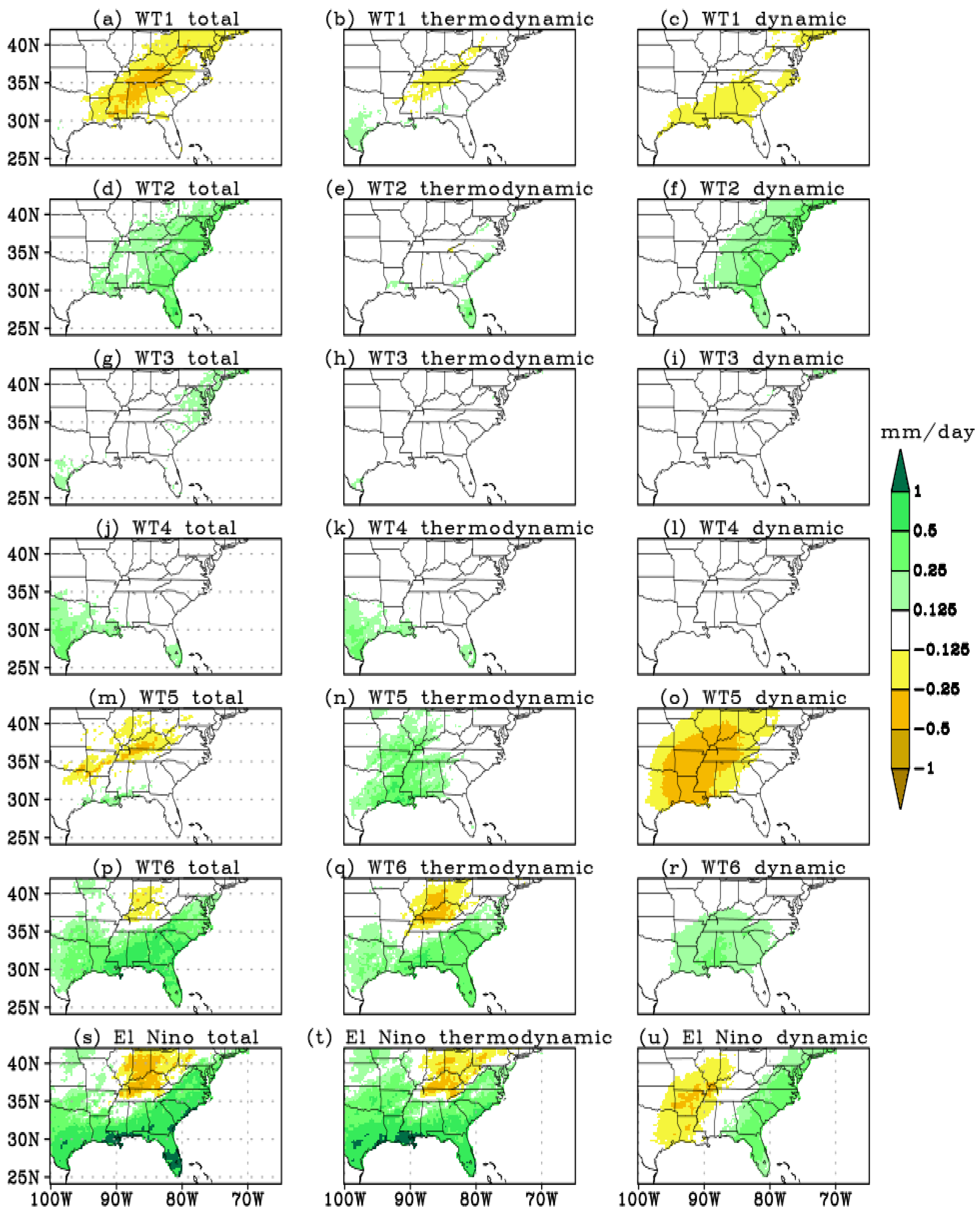
Every term in Equations (2) and (3) is calculated and shown in Figure 8. The thermodynamic contribution (Equation (2)) and dynamic contribution (Equation (3)) to the anomalous precipitation in El Niño years are shown in the middle and right column of Figure 8, respectively, and the sum of the thermodynamic and dynamic contributions by each WT is shown in the left column. The total contribution of the six WTs is shown in the bottom row.
The dynamic contribution (Equation (3)) is approximately the precipitation pattern shown in Figure 3 multiplied by the frequency difference between El Niño years and all years (red and gray bars) in Figure 7. The WTs with a shallow trough (WT1) or a trough of more western location (WT5, WPT) are less frequent, producing negative dynamic contributions from WT1 in the coastal plains and from WT5 in the Mississippi River Valley, respectively (Figure 8c,o). The WTs with deep troughs and more eastern location (WTs 2, 3, and 6) are more frequent in El Niño years. Therefore, positive dynamic contribution is in Eastern US and Southern US in WT2 and WT6, respectively (Figure 8f,r). The precipitation over land is very light in WT3 (Figure 3), so the dynamic contribution to precipitation from WT3 is also very small (Figure 8i). The frequency difference of WT4 is small (Figure 7); thus, the dynamic contribution to anomalous precipitation is small (Figure 8l). Summing up dynamic contribution from all six WTs, the total dynamic contribution to the anomalous precipitation (Figure 8u) features a dipolar pattern of a negative anomaly in the Mississippi River valley versus a positive precipitation anomaly in the east coast states.
The thermodynamic contribution is quite different among the WTs. For each WT, the thermodynamic contribution is also quite different from the corresponding dynamic one. The thermodynamic contribution of WT1 is the negative precipitation anomaly west of the Appalachian Mountain. Therefore, the total contribution of WT1 (Figure 8a) is the southwest–northeast-oriented area of negative anomalous precipitation from the Gulf coast to the Northeast U.S. The thermodynamic contribution of WT2, 3 and 4 is small, except for some localized areas in Florida and Texas. The thermodynamic contribution of WT5 is positive anomalous precipitation in the Gulf coast and Mississippi River Valley region (implying wetter air in El Niño years, Figure 8n), with the opposite sign to the dynamic contribution (Figure 8o). The latter is stronger than the former so that the total contribution of WT5 is the negative anomalous precipitation, extending from northeast Texas to southwest Pennsylvania (Figure 8m). The thermodynamic contribution of WT6 is strong (Figure 8q), with positive anomaly in the Gulf and east coast and negative anomaly in the Ohio River Valley. The combination of thermodynamic and dynamic contributions makes the total contribution of WT6 (Figure 8p) with positive precipitation in all south and east coastal states and negative precipitation anomaly within the Ohio River Valley. The pattern of the total contribution of WT6 (Figure 8p) is quite similar to the total El Niño impact shown in Figure 8s, indicating that most of the precipitation anomaly is contributed by WT6. WT2 increased the positive precipitation anomaly in the east coast, and WT1 and WT5 enhanced the negative precipitation anomaly in the Ohio River Valley.
The relative role of the thermodynamic and dynamic contribution to the precipitation anomaly, in terms of percentage, is location dependent, as seen in Figure 8s–u. For some places, such as Louisiana, the two contributions are opposite in sign. For the east coast, the two contributions both increase precipitation with slightly stronger contribution from the thermodynamic term. In the Gulf coast, the thermodynamic contribution dominates over the dynamic one, especially in the area close to the coast. In the Ohio River valley, both contributions are negative, therefore, reinforcing each other, but the thermodynamic contribution looks stronger than the dynamic one.
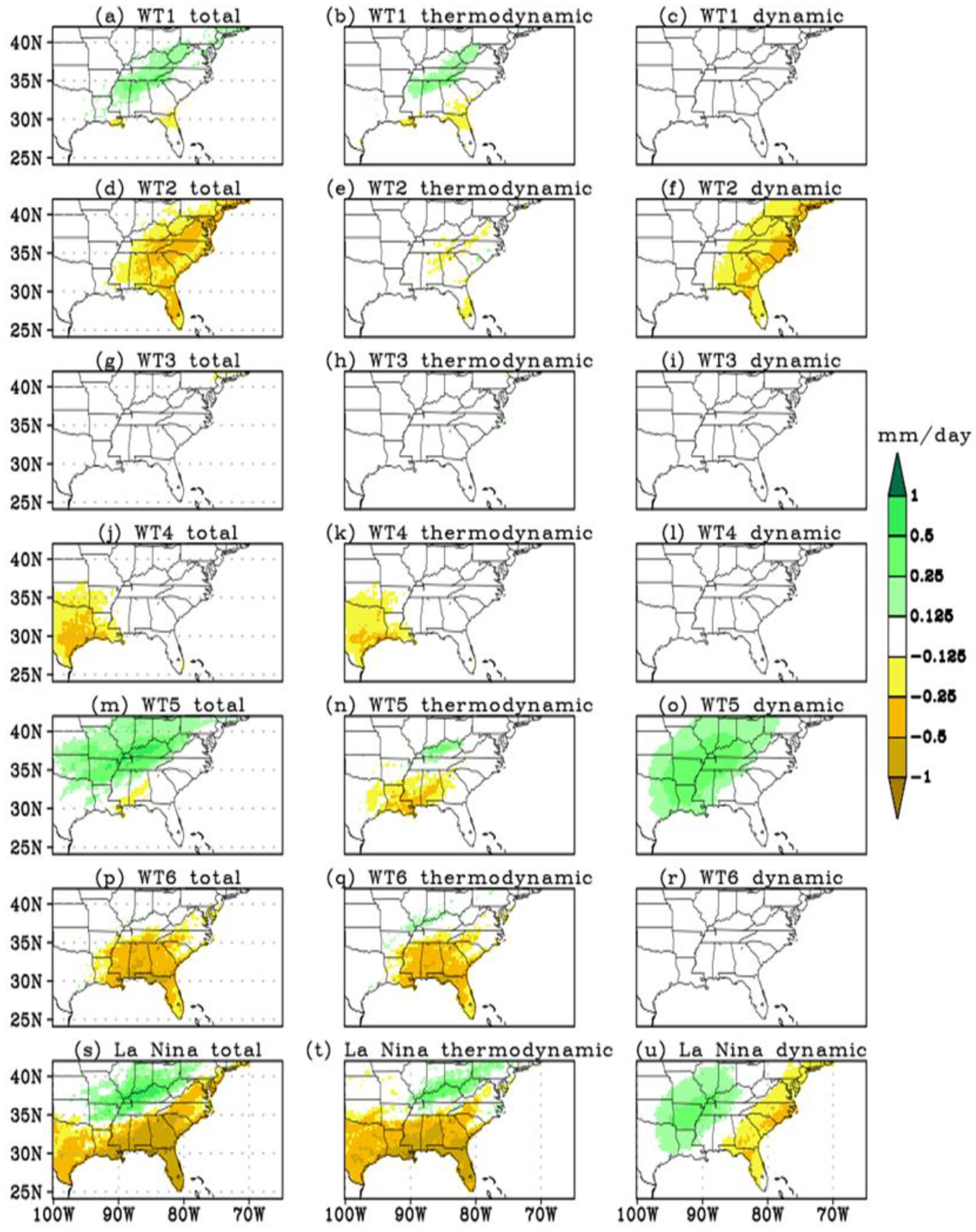
The La Niña impact on the precipitation in the SEUS is shown in Figure 9. The patterns are quite similar to the El Niño impact shown in Figure 8, but with opposite signs. However, there are some asymmetries between the El Niño and La Niña impacts. For example, the dynamic contribution of WT1 is smaller (Figure 9c), the thermodynamic contributions of WT5 seems weaker and less homogeneous (Figure 9n) and both the thermodynamic and dynamic contribution of WT6 are weaker in La Niña than those in El Niño. The area of positive precipitation anomaly in the Ohio River Valley is larger in La Niña (Figure 9s) than that in El Niño (Figure 8s).
The current result is consistent with that of Nieto Ferreira et al. [15] who found stronger mid-latitude cyclones and more intense precipitation over a large area in the SEUS during El Niño than La Niña and normal years. In contrast, negative rainfall anomalies are found in the east coast and Gulf coast areas in the SEUS in La Niña years.

4. Conclusions and Discussion

In order to link weather and climate variability associated with ENSO, we analyzed daily WTs in the SEUS. Six winter weather types were obtained using k-means clustering analysis of the NRP 850 hPa wind components in November to February of 1948–2022. These six WTs have shorter persistence as compared to the summer WTs in [9]. This is because winter weather is mostly controlled by fast propagating westerly waves. A progression loop comprising WTs 2–6 corresponds to the transient westerly waves.
In our previous study, there were six WTs in the long period of eight months from March to October [9]. Here, there are also six WTs in the short period of four months from November to February. The stronger baroclinicity in the winter generates more fast-moving WTs. In contrast, the quasi-stationary NASH produces long-lasting summer WTs.
The frequency and spatial pattern of the WTs can be effectively used to understand the ENSO impact on winter precipitation in the SEUS. We quantified the ENSO impact in terms of dynamic and thermodynamic contribution to anomalous precipitation, respectively. The dynamic contribution is due to the change in the frequencies of the WTs. There are more frequent WTs of deep east coast trough types and plains trough type (WT2, 3 and 6) and less shallow troughs (WT1) and western Plains troughs (WT5) in El Niño years. The more frequent east coast trough and plains trough produce above normal precipitation in southeast coastal plains and Gulf coastal plains. The less frequent WT5 tends to reduce rainfall from the Great Lakes southwestward, producing a negative precipitation anomaly in the Central U.S., south of the Great Lakes. The thermodynamic contribution is from the change in spatial pattern of environmental variables, such as temperature and humidity. In the SEUS, the thermodynamic contribution is as strong as, and even slightly stronger than, the dynamic contribution. Particularly, the thermodynamic term of WT6 makes the largest contribution to the anomalous precipitation associated with El Niño. In general, the thermodynamic and dynamic contribution to the anomalous precipitation in La Niña is quite similar to those in El Niño, but with the opposite sign. However, the influence from WT6 in the La Niña is weaker than that in the El Niño.
Now that we have studied both warm season WTs in March to October [9] and winter WTs in November to February in the current study, respectively, we obtained a quite complete view of the WTs in the whole year. Of course, there are some overlapping WTs between warm season and winter WTs, which may be related to the WTs in the transitioning seasons. We studied the ENSO impact on precipitation from the perspective of the WTs in spring [9] and winter, respectively. It may also be interesting to study the ENSO impacts in the summer and fall using the WTs. Impacts of climate variability on other time scales, such as the intra-seasonal Madden Julian Oscillation and the long-term trend of climate change, also warrant further investigation.

Author Contributions

Conceptualization, J.-H.Q.; Data curation, C.L.; Formal analysis, J.-H.Q. and C.L.; Methodology, J.-H.Q.; Writing—original draft, J.-H.Q.; Writing—review & editing, B.V., S.N. and D.W. All authors have read and agreed to the published version of the manuscript.

Funding

This work was produced by Battelle Savannah River Alliance, LLC under Contract No. 89303321CEM000080 with the U.S. Department of Energy. Publisher acknowledges the U.S. Government license to provide public access under the DOE Public Access Plan (http://energy.gov/downloads/doe-public-access-plan, accessed on 20 July 2022).

Data Availability Statement

The data presented in this study are available on request from the corresponding author. The data are not publicly available due to database access restrictions.

Acknowledgments

We appreciate the constructive comments by the anonymous reviewers, which greatly improved the paper.

Conflicts of Interest

The authors declare no conflict of interest.

References

  1. Ropelewski, C.F.; Halpert, M.S. North American precipitation and temperature patterns associated with the El Niño–Southern Oscillation. Mon. Weather Rev. 1986, 114, 2352–2362. [Google Scholar] [CrossRef] [Green Version]
  2. Roller, C.D.; Qian, J.-H.; Agel, L.; Barlow, M.; Moron, V. Winter weather regimes in the Northeast United States. J. Clim. 2016, 29, 2963–2980. [Google Scholar] [CrossRef]
  3. Nigam, S.; Sengupta, A. The full extent of El Niño’s precipitation influence on the United States and the Americas: The suboptimality of the Niño 3.4 SST index. Geophys. Res. Lett. 2021, 48, e2020GL091447. [Google Scholar] [CrossRef]
  4. Coe, D.; Barlow, M.; Agel, L.; Colby, F.; Skinner, C.; Qian, J.-H. Clustering analysis of autumn weather regimes in the Northeast U.S. J. Clim. 2021, 34, 7587–7605. [Google Scholar] [CrossRef]
  5. Qian, J.-H.; Robertson, A.W.; Moron, V. Interaction among ENSO, the monsoon and diurnal cycle in rainfall variability over Java, Indonesia. J. Atmos. Sci. 2010, 67, 3509–3524. [Google Scholar] [CrossRef]
  6. Qian, J.-H.; Robertson, A.W.; Moron, V. Diurnal cycle in different weather regimes and rainfall variability over Borneo associated with ENSO. J. Clim. 2013, 26, 1772–1790. [Google Scholar] [CrossRef]
  7. Qian, J.-H. Mechanisms for the dipolar patterns of rainfall variability over large islands in the Maritime Continent associated with the Madden-Julian Oscillation. J. Atmos. Sci. 2020, 77, 2257–2278. [Google Scholar] [CrossRef]
  8. Ohba, M.; Nohara, D.; Yoshida, Y.; Kadokura, S.; Toyoda, Y. Anomalous weather patterns in relation to heavy precipitation events in Japan during the Baiu season. J. Hydrometeorol. 2015, 16, 688–701. [Google Scholar] [CrossRef]
  9. Qian, J.-H.; Viner, B.; Noble, S.; Werth, D. Precipitation characteristics of warm season weather types in the southeastern United States of America. Atmosphere 2021, 12, 1001. [Google Scholar] [CrossRef]
  10. Bell, G.D.; Bozart, L.F. Appalachian cold-air damming. Mon. Weather Rev. 1988, 116, 137–161. [Google Scholar] [CrossRef] [Green Version]
  11. Rackley, J.A.; Knox, J.A. A climatology of southern Appalachian cold-air damming. Weather. Forecast. 2016, 31, 419–432. [Google Scholar] [CrossRef]
  12. Kalnay, E.; Kanamitsu, M.; Kistler, R.; Collins, W.; Deaven, D.; Gandin, L.; Iredell, M.; Saha, S.; White, G.; Woollen, J.; et al. The NCEP/NCAR 40-year reanalysis project. Bull. Amer. Meteor. Soc. 1996, 77, 437–471. [Google Scholar] [CrossRef] [Green Version]
  13. Xie, P.; Joyce, R.; Wu, S.; Yoo, S.-H.; Yarosh, Y.; Sun, F.; Lin, R. Reprocessed, bias-corrected CMORPH global high-resolution precipitation estimates from 1998. J. Hydrometeorol. 2017, 18, 1617–1641. [Google Scholar] [CrossRef]
  14. Ohba, M.; Sugimoto, S. Dynamic and thermodynamic contributions of ENSO to winter precipitation in Japan: Frequency and precipitation of synoptic weather patterns. Clim. Dyn. 2021, 1–16. [Google Scholar] [CrossRef]
  15. Nieto Ferreira, R.; Hall, L.; Richenbach, T.M. A climatology of the structure, evolution, and propagation of midlatitude cyclones in the Southeast United States. J. Clim. 2013, 26, 8406–8421. [Google Scholar] [CrossRef]
Figure 1. Monthly climatology of precipitation (shades, mm/day) and 850 hPa horizontal circulation (arrows, m/s) in winter in the Southeast U.S. The mean winds are based on the NRP reanalysis of 1948–2022. The mean precipitation is based on the CMORPH (NOAA Climate Prediction Center-CPC Morphing Technique) satellite estimated data for 1998–2020.
Atmosphere 13 01159 g001
Figure 2. The classifiability index (CI) of the k-means clustering analysis using 850 hPa zonal and meridional wind component (u and v) in the Southeast U.S. and the surrounding region (100–65° W, 20–45° N) in the winter months (November–February) of 1948–2022; the optimum number for the k-means analysis is k = 6.
Atmosphere 13 01159 g002
Figure 3. The average precipitation (shade, mm/day) and 850 hPa winds (arrows) of the six WTs. WTs 1–6 can be briefly described as Shallow Trough (ST), East Coast Trough (ECT), Off East Coast Trough (OECT), Mississippi River Valley Ridge (MRVR), Western Plains Trough (WPT) and Plains Trough (PT), respectively.
Atmosphere 13 01159 g003
Figure 4. The daily weather types (WTs) in the winter of 1948–2022 (top). The 74-year averaged frequency (percentage) of the 6 WTs from November 1 to February 28 (120 days/year); a 5-day running average was conducted (bottom). Color: WT1 (pink), WT2 (purple), WT3 (light blue), WT4 (green), WT5 (yellow), WT6 (red).
Atmosphere 13 01159 g004
Figure 5. Persistence of the 6 WTs presented by different color bars, respectively. The x-axis is the length of consecutive days with the same WT. The last group of bars is the sums of persistent events of 6 to 12 days.
Atmosphere 13 01159 g005
Figure 6. The progression of the WTs. The 95% confidence interval of the WT background frequency (the occurrence of WT transition due to chance) is shown with black shading. Frequencies significantly greater than the background frequency are shown with red bars; frequencies significantly less than the background bars are shown with blue bars.
Atmosphere 13 01159 g006
Figure 7. Frequencies of the WTs in all years (grey), El Niño years (red) and La Niña years (green) in December–February of the ENSO years.
Atmosphere 13 01159 g007
Figure 8. Precipitation anomalies in El Niño years in December–February (panel (s)). Panels (ar) are the contribution of the WTs 1–6 to the anomalous precipitation. Left, middle and right panels are the total, thermodynamic and dynamic contribution from each WT, respectively. Panels (t,u) are the sum of thermodynamic and dynamic contribution for all WTs, respectively.
Atmosphere 13 01159 g008
Figure 9. Precipitation anomalies in La Niña years in December–February (panel (s)). Panels (ar) are the contribution of the WTs 1–6 to the anomalous precipitation. Left, middle and right panels are the total, thermodynamic and dynamic contribution from each WT, respectively. Panels (t,u) are the sum of thermodynamic and dynamic contribution for all WTs, respectively.
Atmosphere 13 01159 g009
Table 1. Six weather types in the winter and their 850 hPa flow patterns.
Weather TypeDescription
WT1Shallow trough (ST) over central-east US
WT2East coast trough (ECT)
WT3Off-east-coast trough (OECT)
WT4Mississippi River Valley Ridge (MRVR)
WT5Western plains trough (WPT)/Off coast Carolina high (OCCH)
WT6Plains trough (PT)
Publisher’s Note: MDPI stays neutral with regard to jurisdictional claims in published maps and institutional affiliations.

