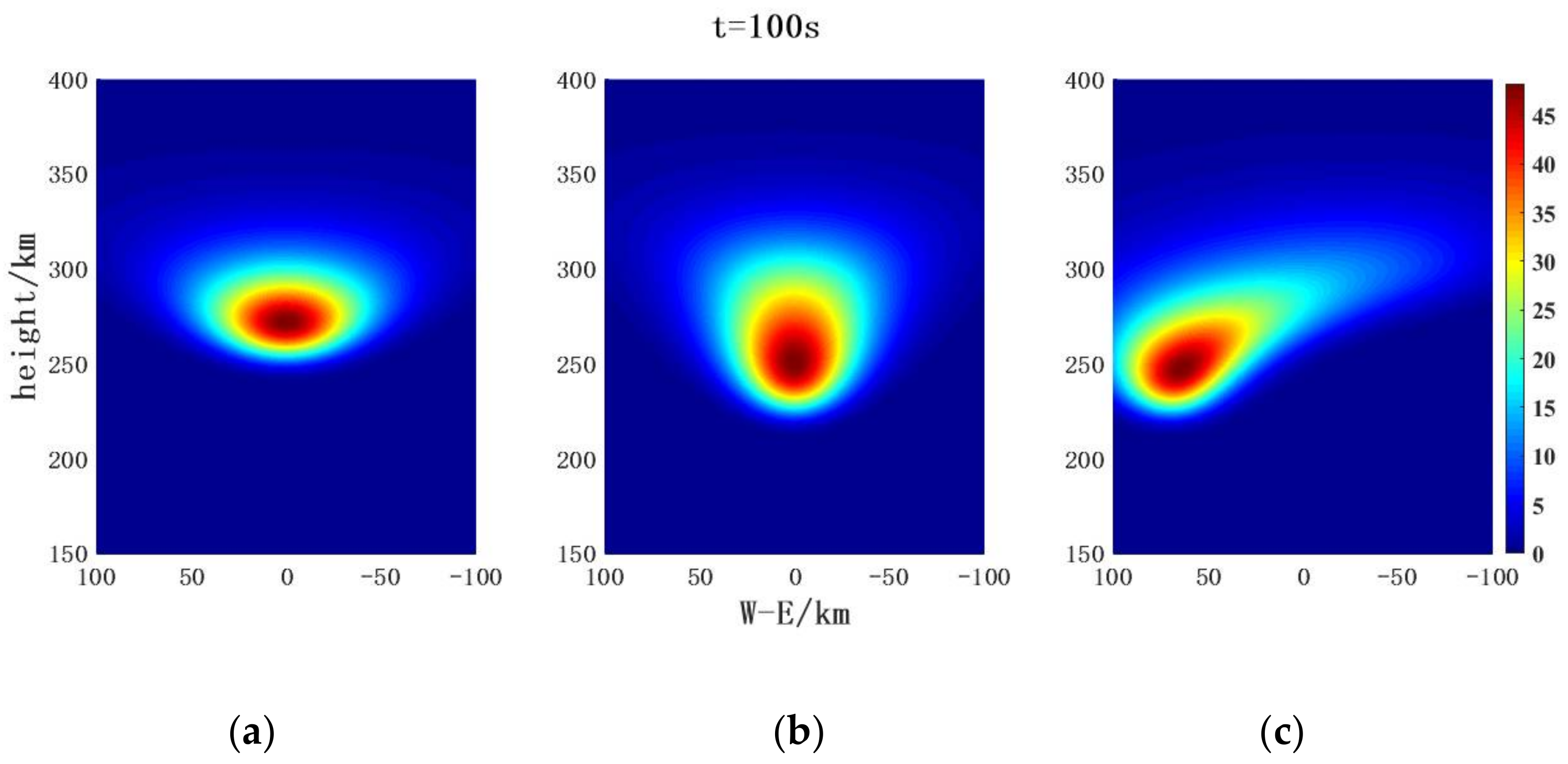
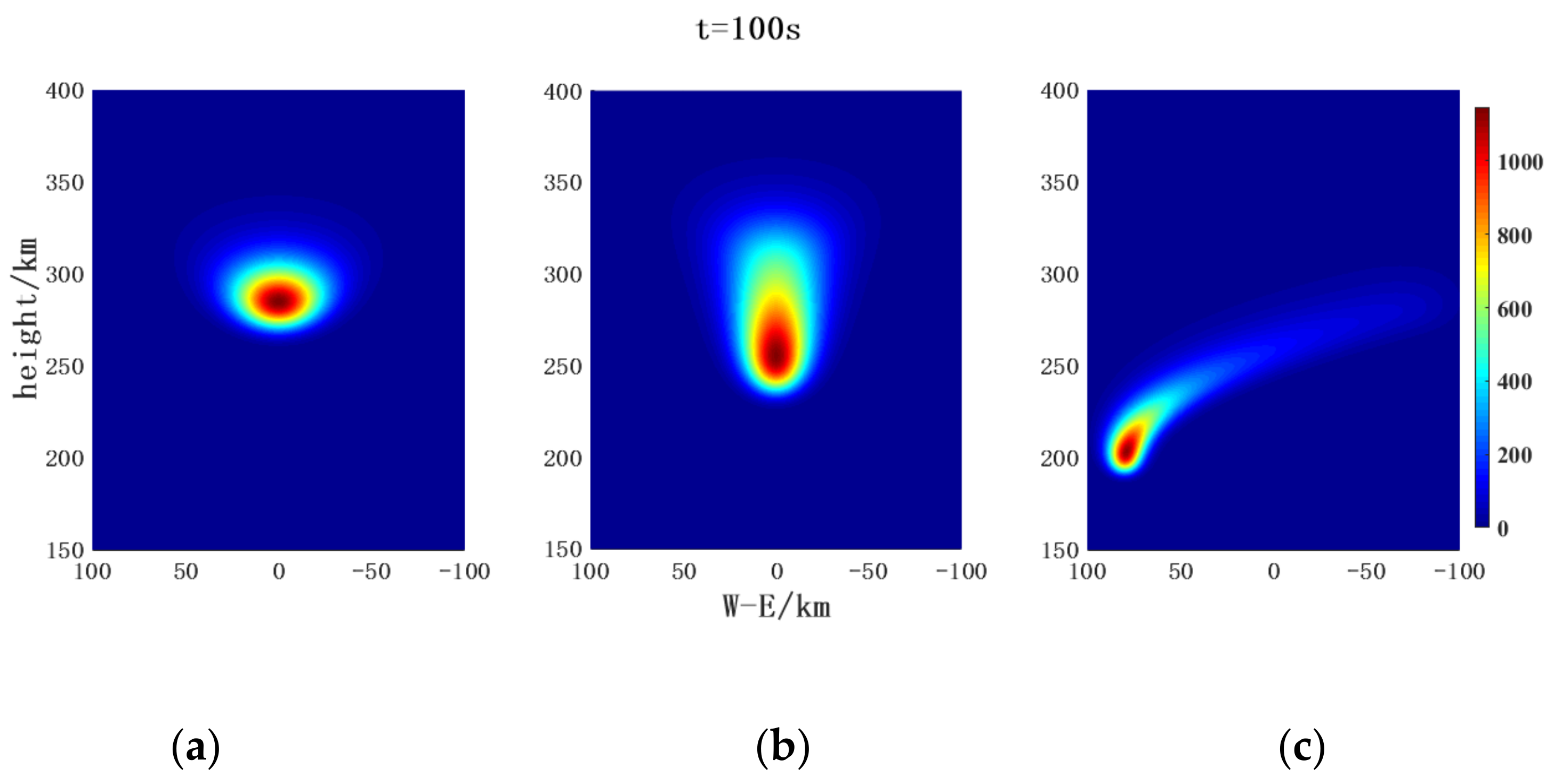
4.2.1. Simulation of Spatial Distribution of H2O after Release and Diffusion in Different Paths
As shown in
Figure 7, after releasing H
2O for 100 s according to fixed-point release of 300 km, vertical path release of 250–350 km and parabolic curve path of 250–350 km, the released substance H
2O has different spatial distribution characteristics. Similar to the case of H
2 under three different release paths, when it is released at a fixed point of 300 km, the east–west diffusion of H
2O is farther than the vertical height, so a flat ellipsoidal release space is also generated; when the 250–350 km vertical path is released, the east–west diffusion of the release substance is smaller than the vertical diffusion, resulting in a slender cylindrical diffusion space with narrow bottom and wide top; when released on a parabolic path of 250–350 km, a parabolic tubular release space is generated. Different from the diffusion of H
2 under three different release paths, the diffusion range of H
2 is greater than that of H
2O after 100 s of release, because the molecular weight and collision cross-sectional area of H
2 are small, so the diffusion rate of H
2 is higher than that of H
2O.
4.2.2. Ionospheric Disturbance Released by H2O in Different Paths and Its Influence on Radio Wave Propagation Path
Similarly, we simulated the ionospheric disturbance caused by H
2O under three different release paths and its impact on the radar wave propagation path. The simulation results are shown in
Figure 8,
Figure 9,
Figure 10 and
Figure 11.
Figure 8,
Figure 9,
Figure 10 and
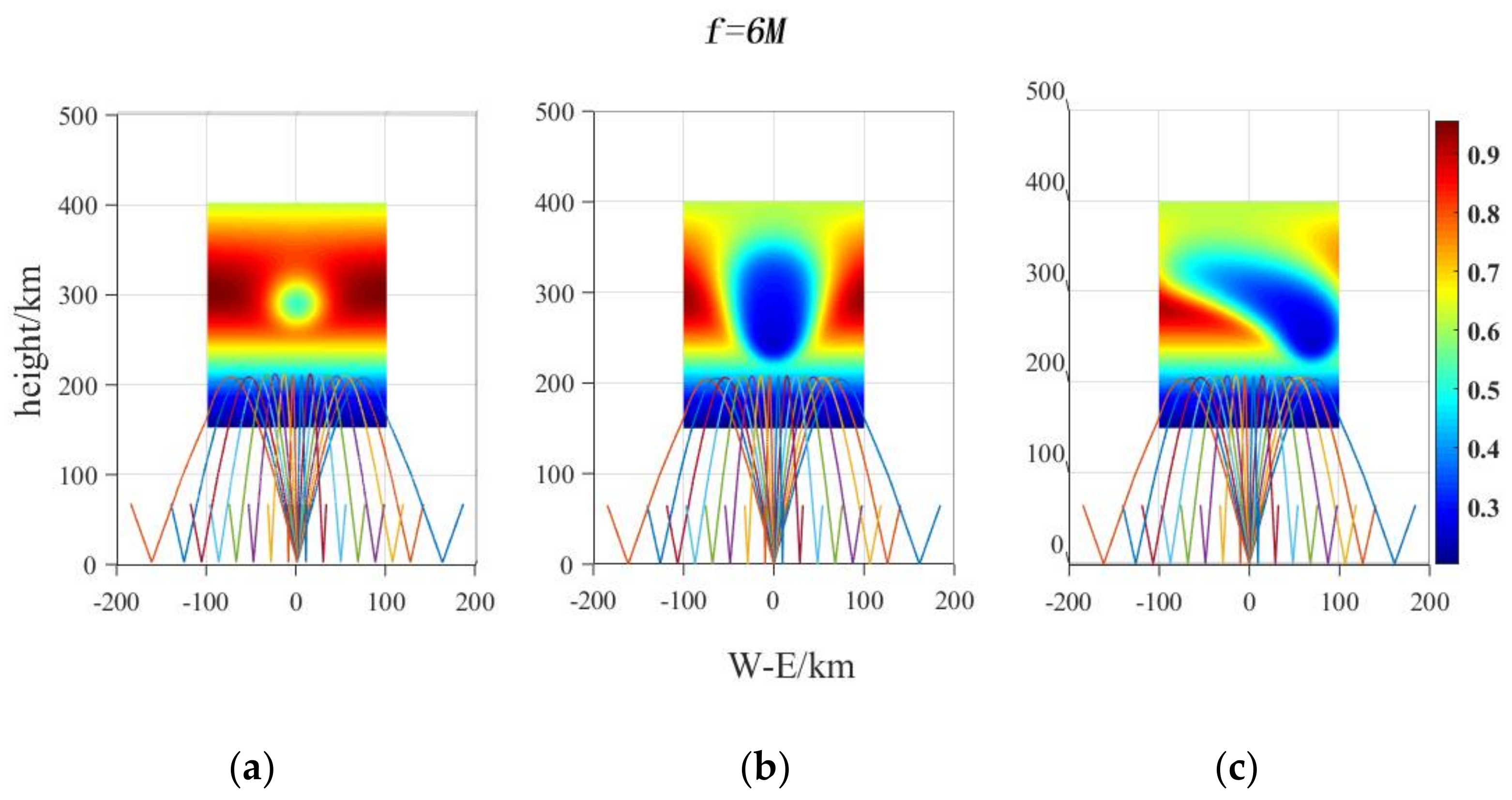
Figure 11a–c shows the ionospheric disturbance generated by the rocket after releasing H
2O for 100 s under different flight paths (i.e., fixed-point release at 300 km; vertical path at 250–350 km; parabola path at 250–350 km) and its impact on radar wave propagation at different frequencies. Similar to the ionospheric disturbance generated by H
2 under the same release path, an ellipsoidal ionospheric cavity is generated after releasing 3000 mol H
2O at a fixed point of 300 km for 100 s. After releasing 3000 mol H
2O every 5 km in the vertical direction from 250 km to 350 km for 100 s, a spindle ionospheric cavity is generated. After releasing 3000 mol H
2O for 100 s on the parabolic curve path from 250 km to 350 km, a parabolic-like ionospheric cavity structure is generated. Compared with the ionospheric disturbance generated by H
2 under the same release path, the basic shape of the ionospheric cavity generated by H
2O under the same release path is essentially consistent with the ionospheric disturbance generated by releasing H
2. However, the ionospheric disturbance range produced by H
2 is larger than that produced by H
2O. The dissipation degree of ionospheric electron density caused by the release of H
2O is higher than that produced by H
2, and the maximum relative change rate of electron density is greater. In addition, the boundary of the ionospheric cavity produced by the release of H
2O is clearer and less gradual than that produced by the release of H
2, while the level of electron density disturbance at the boundary is not very obvious.
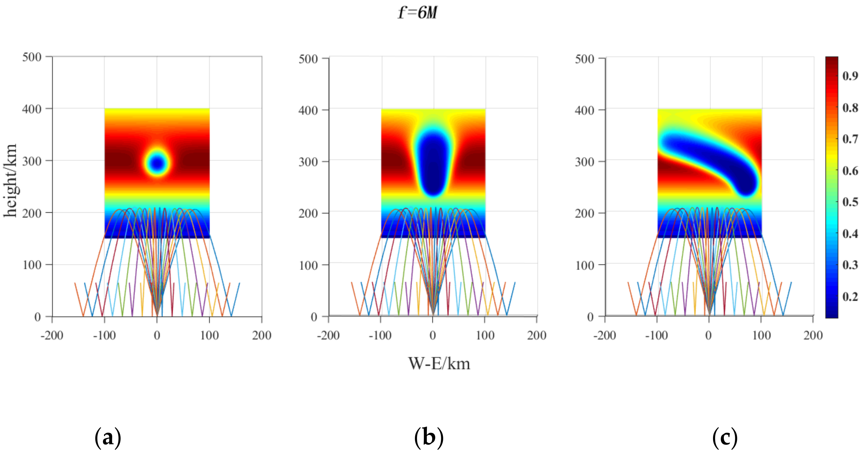
Aiming at the different ionospheric cavity disturbance forms under different release paths, the influence of different ionospheric cavity disturbance forms on the radio wave propagation of sky wave radar is simulated by using three-dimensional ray-tracing technology. As shown in
Figure 8a–c, it is also similar to the case of H
2 release under different paths. Because the frequency of 6 MHz short wave is small and less than the critical frequency of the lower boundary of the cavity, all 6 MHz short waves are reflected back to the ground without reaching the height of the ionospheric disturbance area after incident. The three different forms of ionospheric cavity disturbances produced by the release of H
2O also have no effect on the propagation of 6 MHz short wave.
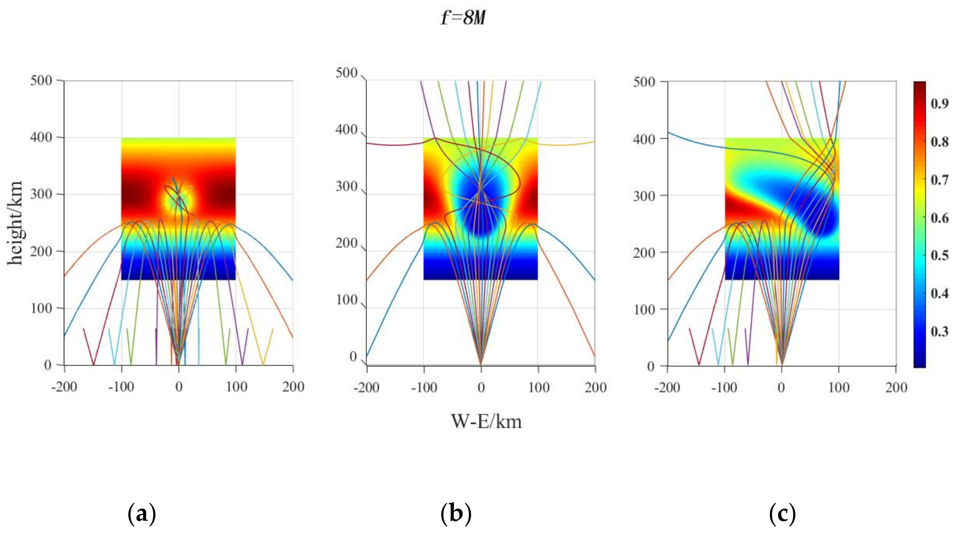
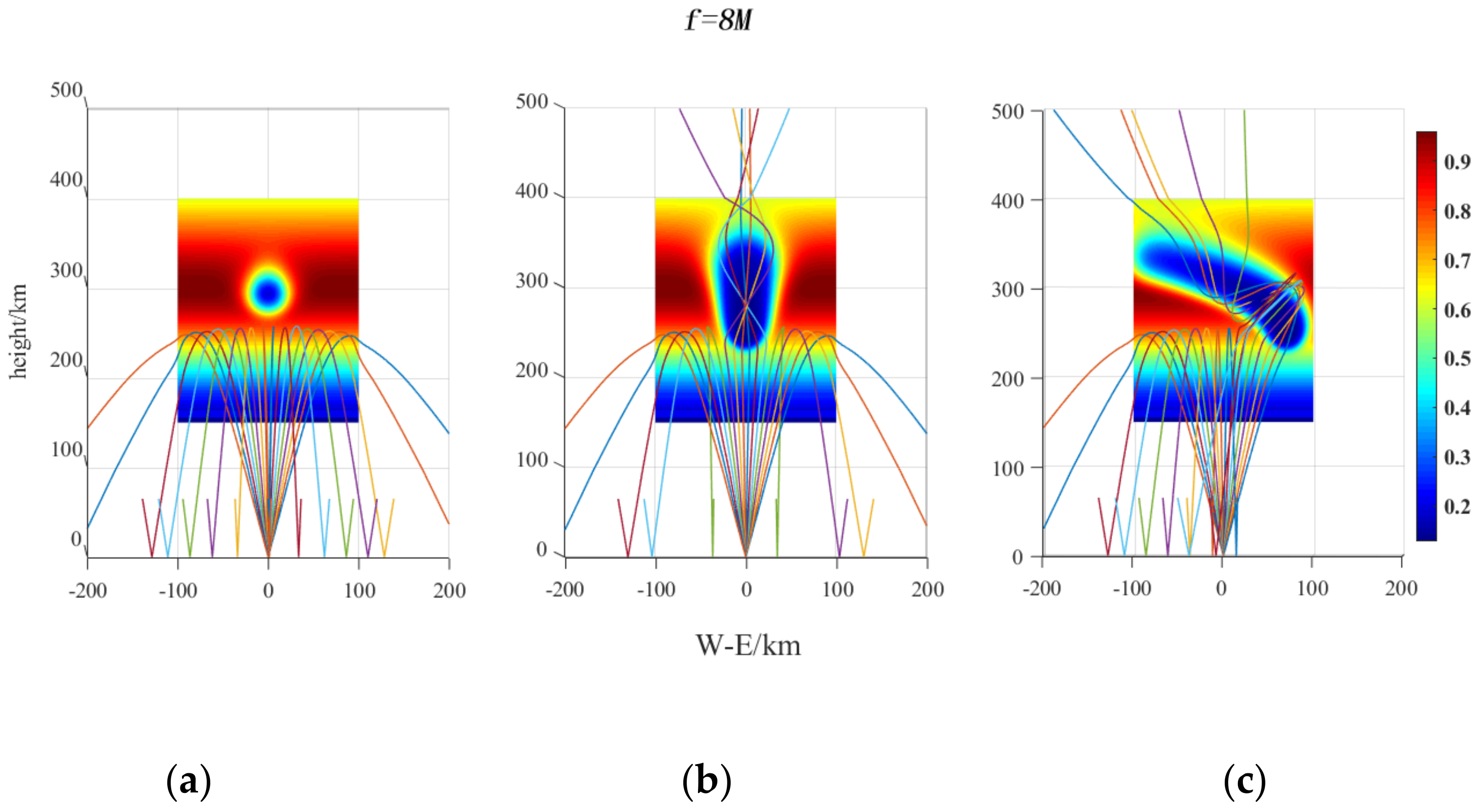
For the propagation path of 8 MHz short wave, it can be seen from
Figure 9a that in contrast with the case of releasing H
2 at a fixed point of 300 km, when releasing H
2O at a fixed point of 300 km, due to the slow diffusion rate of H
2O and small disturbance range, 8 MHz short wave is reflected back to the ground without reaching the lower boundary of ionospheric cavity. It can be seen from
Figure 9b, in contrast with the case of releasing H
2 in the vertical path, due to the slow diffusion rate of released H
2O and small disturbance range, only the 8 MHz beam with the elevation angle closest to 90° can pass through the ionospheric cavity, while most 8 MHz short-wave beams are reflected back to the ground without reaching the ionospheric disturbance area. Compared with
Figure 4c and
Figure 9c, when the parabolic path is released, the propagation path of 8 MHz short wave beam is also different because the diffusion rate of released H
2O is slow and the disturbance range is small, but the electron density dissipation degree is deep and the electron density gradient is large.
Figure 9c shows the influence of the parabolic ionospheric cavity on the 8 MHz short wave propagation. The beam propagation presents obvious asymmetric characteristics. The 8 MHz short wave beam in the east of the emission point passes through the ionospheric cavity after multiple reflections at the inner boundary of the parabolic ionospheric cavity and changes the propagation direction of the radio wave to a great extent. All beams in the west of the transmitting point do not reach the disturbance area and are directly reflected back to the ground.
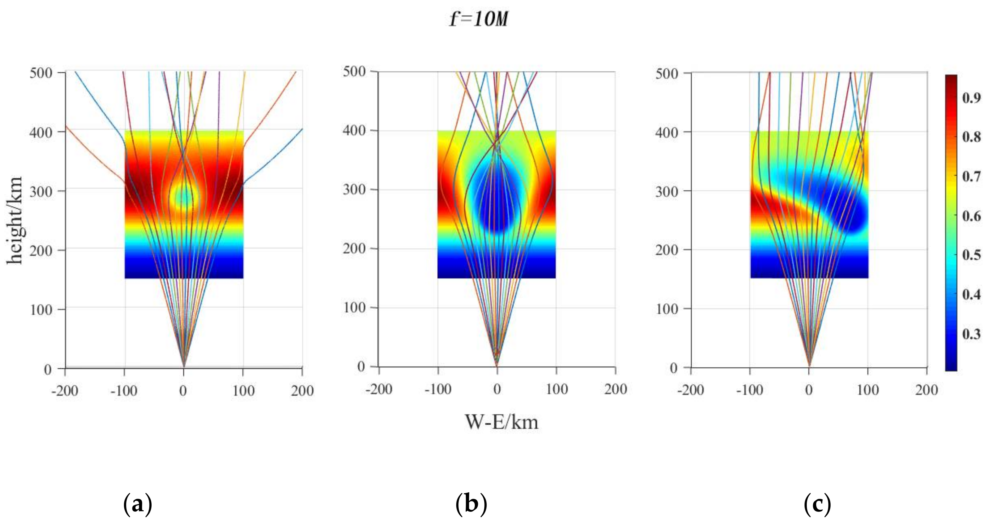
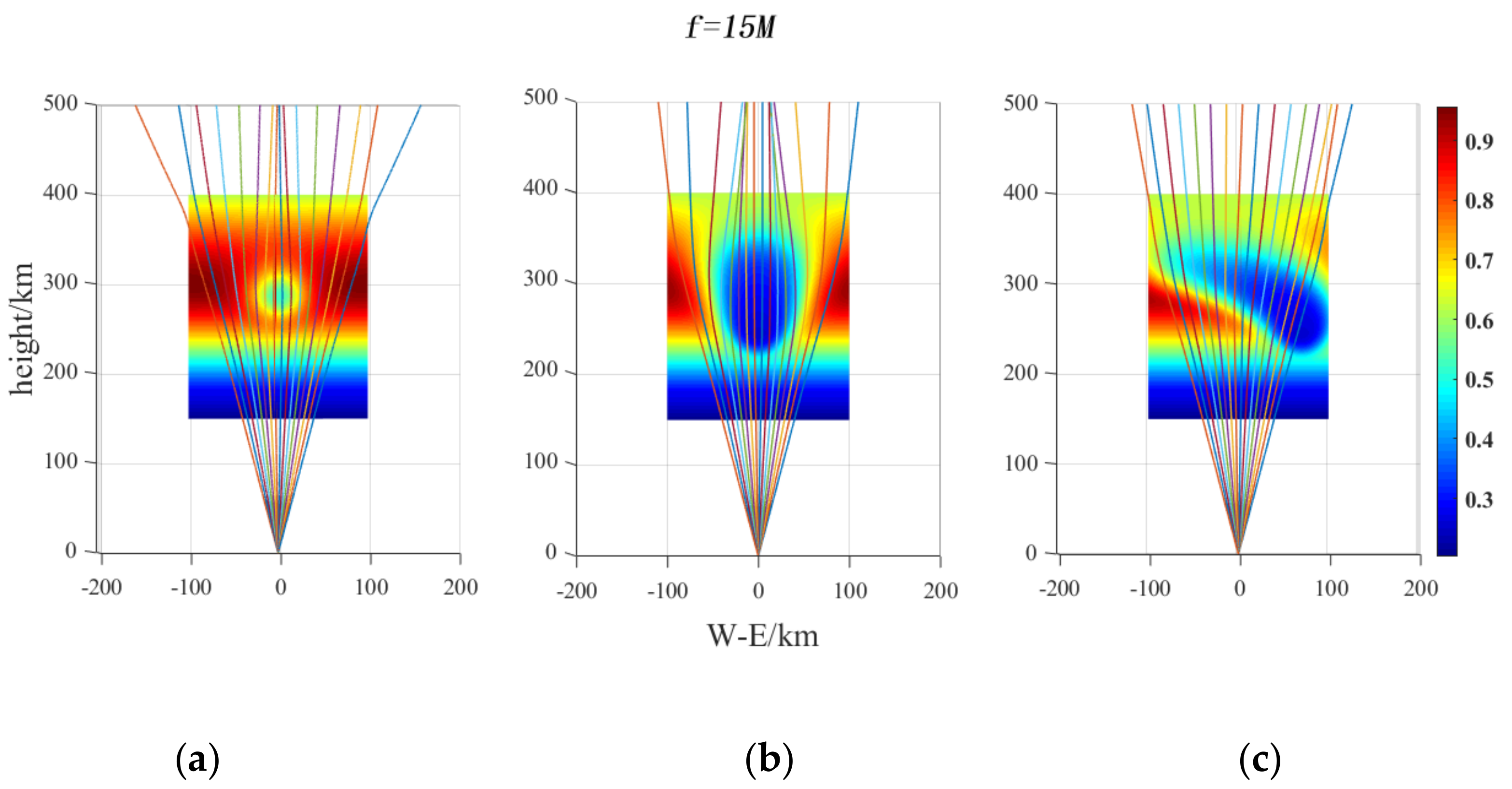
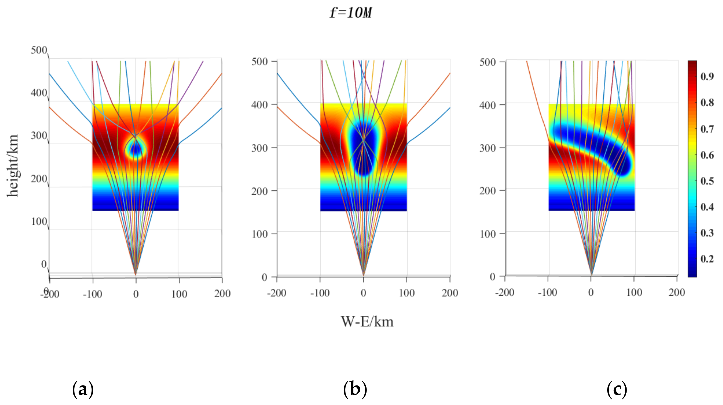
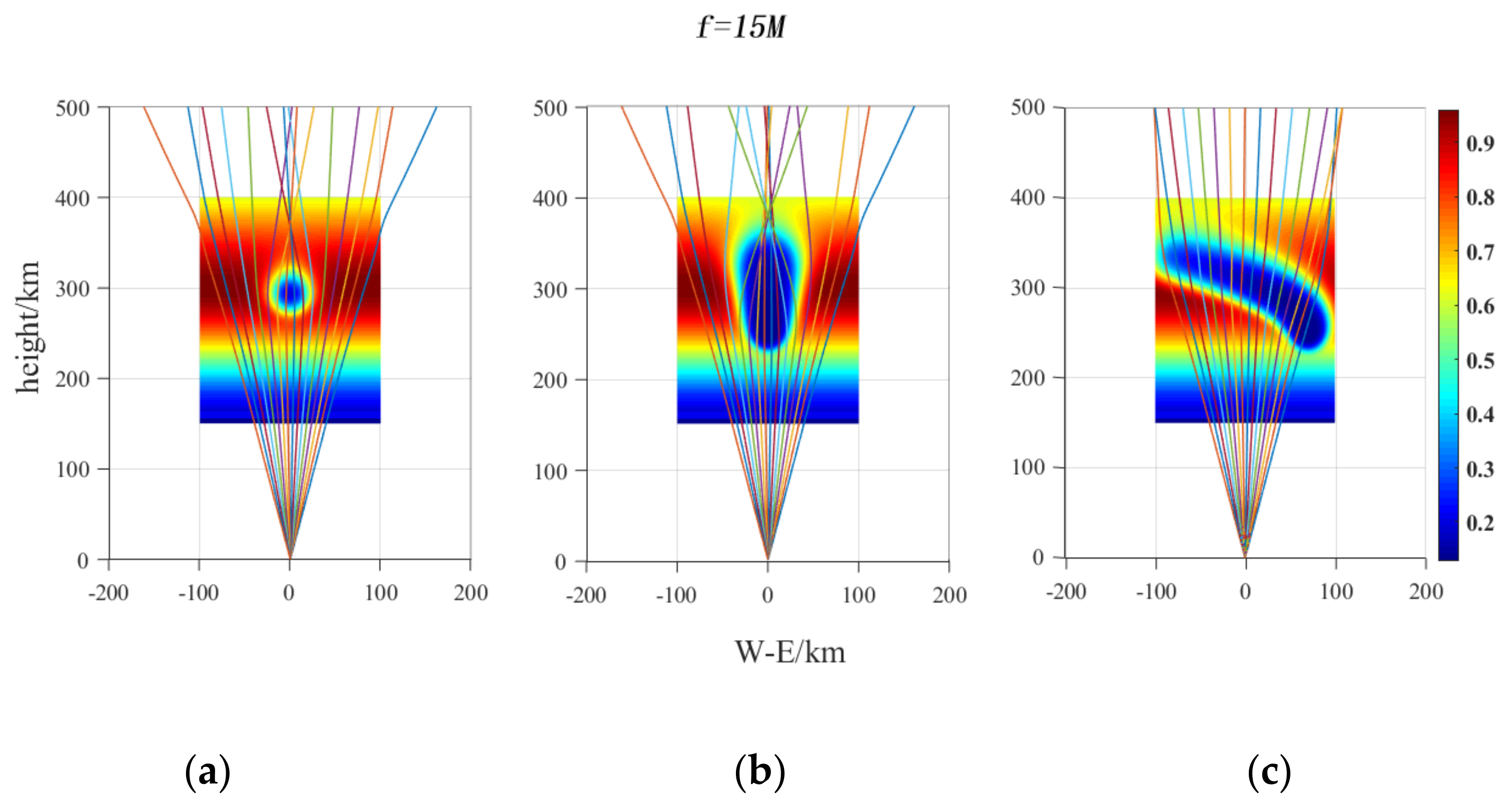
Figure 10 and
Figure 11a–c show the propagation paths of 10 MHz and 15 MHz short waves, which are also similar to the influence of three different forms of ionospheric cavity disturbance generated when H
2 is released on 10 MHz and 15 MHz short waves under the same conditions. The beams of the two frequencies completely pass through the ionospheric disturbance area and have different degrees of focusing effect. Similar to the case of H
2 release, the ionospheric disturbance area generated during vertical release affects the most beams, the focusing effect of radio waves is the strongest and the fixed-point release is the second, while the parabolic release is the weakest. The focusing effect decreases with the increase in the incident frequency, and the corresponding focus increases with the increase in the incident frequency.


