3.2.1. Single Covariate Models
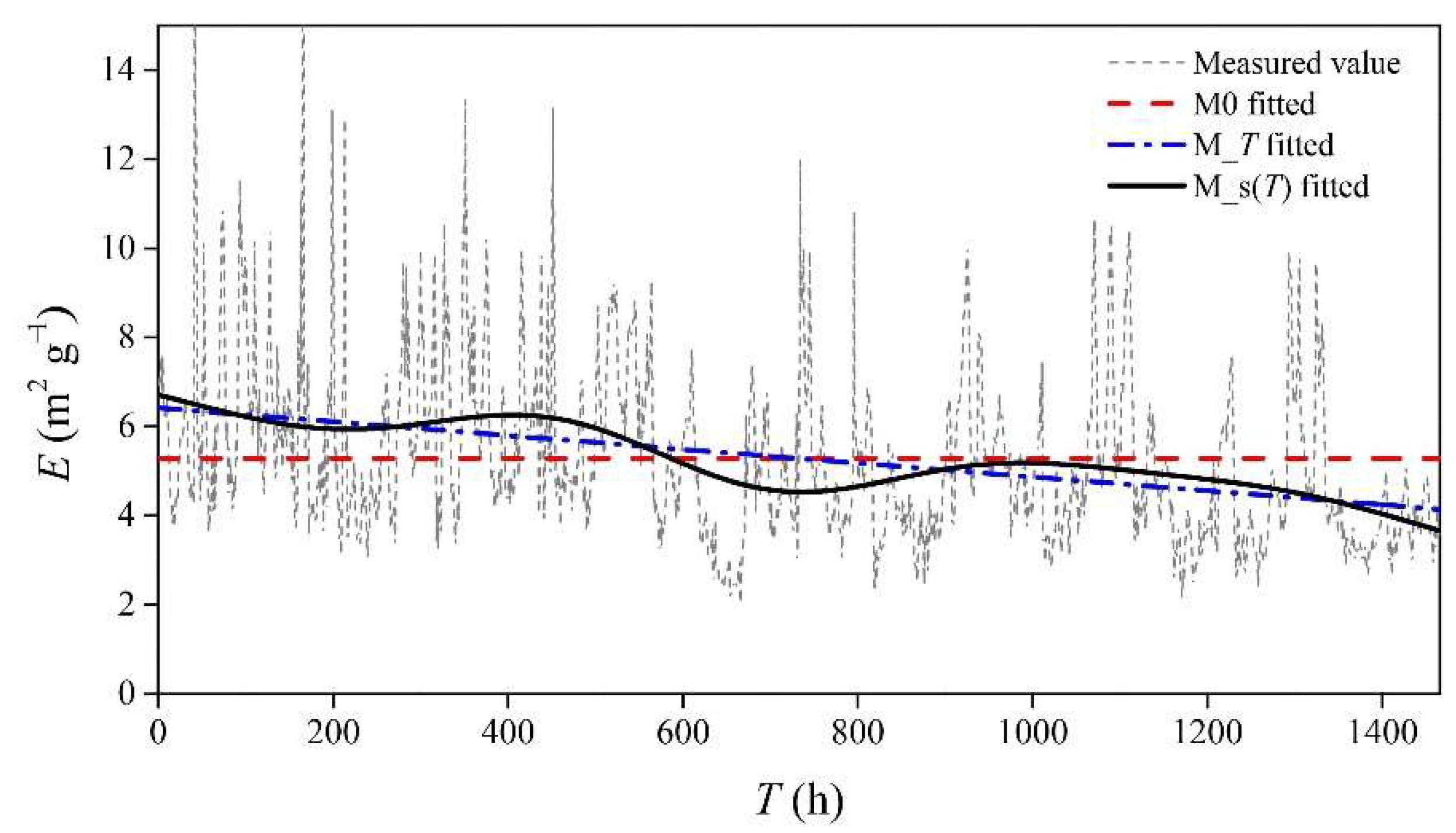
From the fitting results of the nonlinear time-varying model in
Section 3.1, it can be seen that the R
2 and explained variance of the model are only 0.13 and 17.3%, respectively, indicating that the variable
T does not have the best explanatory effect on the non-stationary change of the aerosol extinction coefficient per unit of mass. Therefore, this study introduces environmental meteorological factors RH,
ρBC/
ρPM1,
ρBC/
ρPM2.5,
ρBC/
ρPM10,
ρPM1/
ρPM2.5,
ρPM1/
ρPM10 and
ρPM2.5/
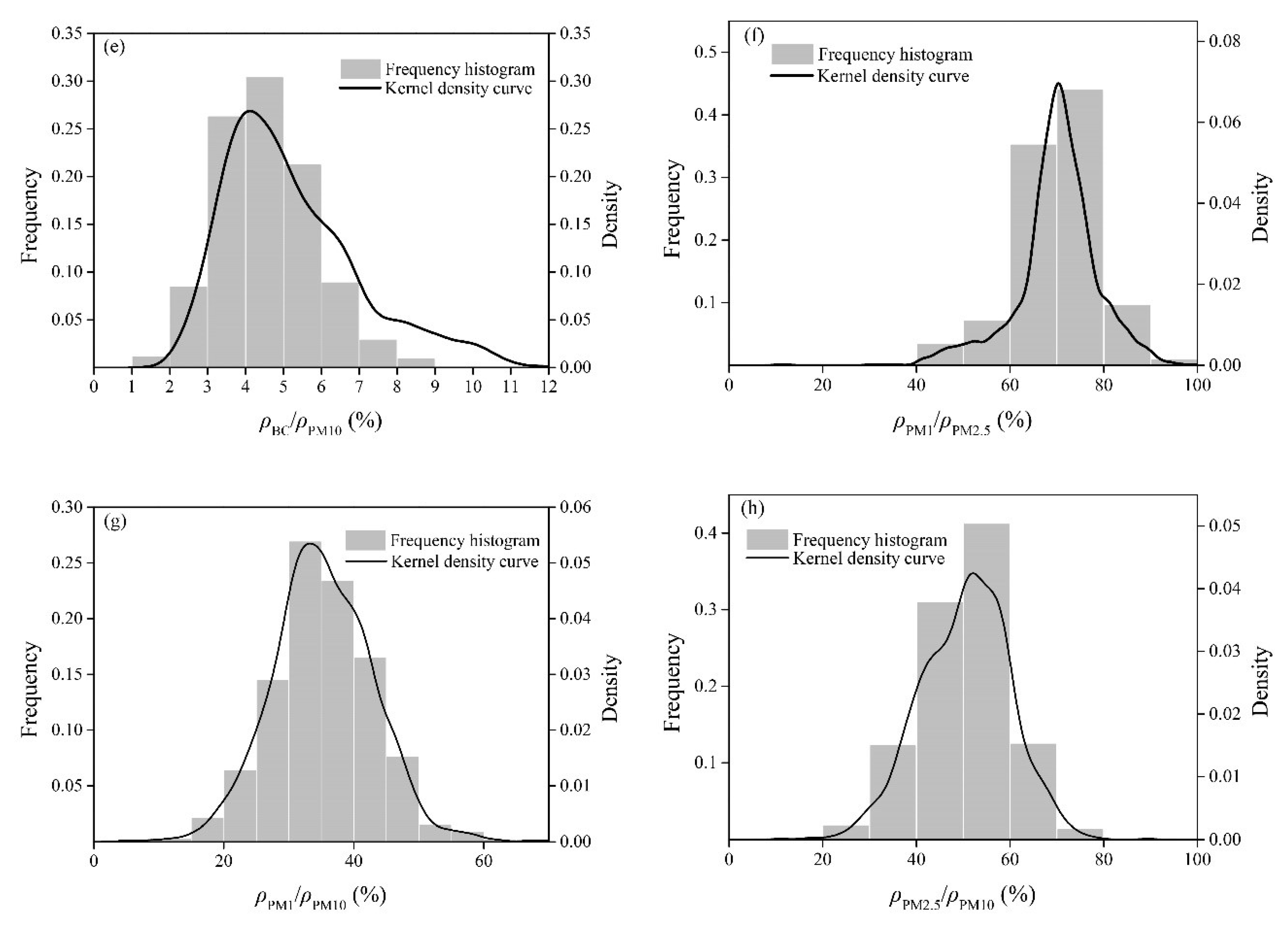
ρPM10 as initial explanatory variables to discuss the causes for the nonstationarity of the aerosol extinction coefficient per unit of mass. Due to the selection of many initial explanatory variables, there may be a problem of collinearity among the variables. This study uses the variance expansion factor (VIF) to analyze the multicollinearity of the variables and eliminates the explanatory variables with multicollinearity [
48]. When the value of VIF is closer to 1, the multicollinearity is lighter, and vice versa. Therefore, the VIF of the final selection factor in this study does not exceed 3. Studies have shown [
49] that
ρBC/
ρPM10,
ρPM1/
ρPM2.5 and
ρPM2.5/
ρPM10 have a certain correlation with the equivalent complex refractive index of aerosols, so the environmental meteorological factors of
ρBC/
ρPM10,
ρPM1/
ρPM2.5 and
ρPM2.5/
ρPM10 are retained. According to the diagnosis results of VIF (
Table 2), the collinearity among the explanatory variables is reduced, and four factors of RH,
ρBC/
ρPM10,
ρPM1/
ρPM2.5 and
ρPM2.5/
ρPM10 are selected as the explanatory variables of the aerosol extinction coefficient per unit of mass. Among these factors, the maximum VIF is 1.73.
The aerosol extinction coefficient per unit of mass is used as the response variable, and one of the above four environmental meteorological factors is selected as an explanatory variable each time to establish a GAMs. The individual influence of each environmental meteorological factor is analyzed in
Table 3. As can be seen, each explanatory variable has a significant impact on the aerosol extinction coefficient per unit of mass (passing the significance test of
α = 0.01), The Edf of each variable is greater than 1, indicating a significant non-linear relationship between the aerosol extinction coefficient per unit of mass and these four environmental meteorological factors. Seen from
Table 3, RH has the greatest influence on the change of aerosol extinction coefficient per unit of mass, and the influence of the aerosol component structure factors is relatively small.
3.2.2. Multiple Covariate Models
Furthermore, a multiple covariate non-stationary model is established based on the environmental meteorological factors. The AIC values of the stationary model, the time-varying non-stationary model and the non-stationary model based on the environmental meteorological factors are shown in
Figure 5. The AIC value of the non-stationary model with the explanatory variable of RH is small and has a better-fitting effect. After adding the aerosol component structure factors, the AIC value of the multiple covariate model (M_multi) is reduced to the lowest. This shows that the RH plays an important role in the change of the aerosol extinction coefficient per unit of mass, but the role of the aerosol component structure factors cannot be ignored.
Table 4 shows the fitting results of the multiple covariate model, and the four environmental meteorological factors all pass the significance test of
α = 0.05. As the Edf of each variable is greater than 1, there is a nonlinear relationship between the aerosol extinction coefficient per unit of mass and the four environmental meteorological factors. By comparing the statistical values of each variable F, it can be concluded that the sequence of the influence of each covariate on the aerosol extinction coefficient per unit of mass is as follows: RH >
ρBC/
ρPM10 >
ρPM2.5/
ρPM10 >
ρPM1/
ρPM2.5. The R
2 and explained variance of the model are 0.67 and 77.90%, respectively, both of which are much larger than those of the time-varying non-stationary model. This shows that the environmental meteorological factors can better characterize the non-stationary changes of the aerosol extinction coefficient per unit of mass than the time variable.
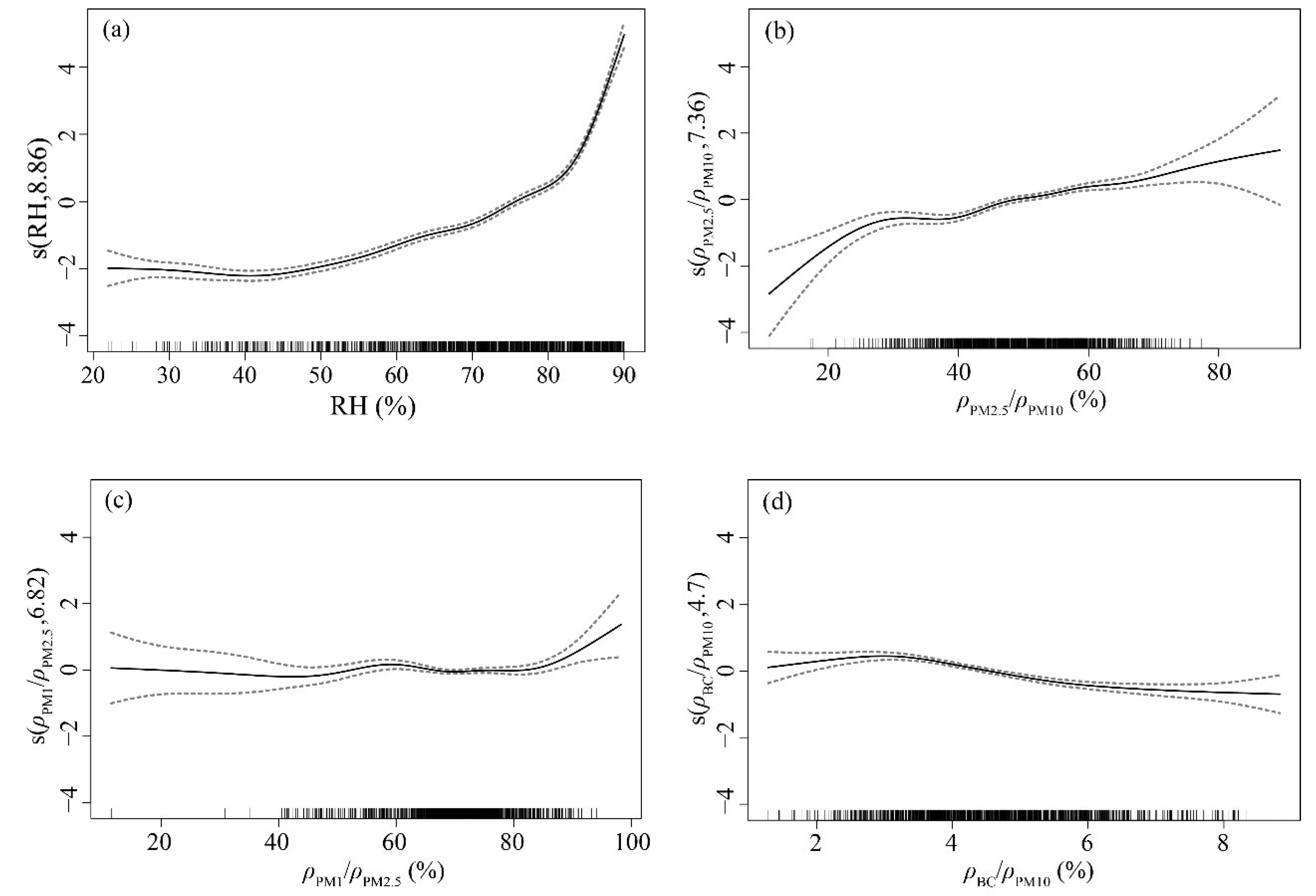
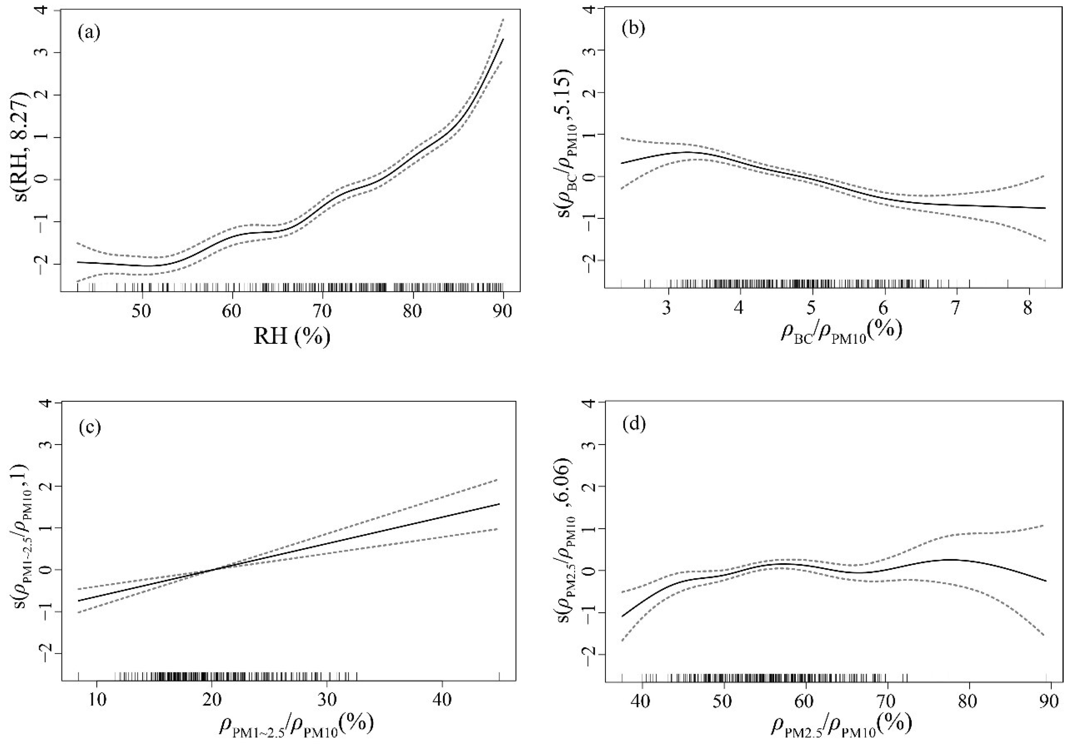
Through the established multiple covariate model, the response graph for the influence of each covariate on the aerosol extinction coefficient per unit of mass is obtained and visually displayed in
Figure 6. As can be seen in
Figure 6, the dotted line represents the upper and lower limits of the confidence level; the solid line represents the smooth curve of the aerosol extinction coefficient per unit of mass based on the explanatory variable; the x-axis represents the measured value of the explanatory variable; the y-axis represents the smooth-simulated value of the aerosol extinction coefficient per unit of mass, and the value in parenthesis on the y-axis represents the estimated degree of freedom. In
Figure 6a it indicates that the aerosol extinction coefficient per unit of mass has a non-linear positive correlation with the RH. When the RH > 80%, the aerosol extinction coefficient per unit of mass increases rapidly with the RH. This is consistent with the research results of Liu et al. and Chen et al. [
50].
Figure 6b indicates the nonlinear relationship that the aerosol extinction coefficient per unit of mass increases with
ρPM2.5/
ρPM10. The proportion of organic carbon, sulfate and nitrate in PM
2.5 in the Chengdu area is relatively large. The increase in the proportion of fine particles in coarse particles leads to the increase of aerosol hygroscopicity, so the aerosol extinction coefficient per unit of mass increases [
51]. In
Figure 6c, the aerosol extinction coefficient per unit of mass changes more slowly with the increase of
ρPM1/
ρPM2.5. In
Figure 6d, the aerosol extinction coefficient per unit of mass decreases with the increase of
ρBC/
ρPM10. This may be related to the non-hygroscopicity of BC and the mixed state of BC [
52]. Due to the absorbability of BC, it can adsorb a large amount of sulfate, nitrate, etc., thereby increasing the size of aerosol particles. According to the condensation growth formula, the larger the particle is, the slower the growth process of particle size [
53]. Therefore, it affects the hygroscopic growth of aerosol particles.
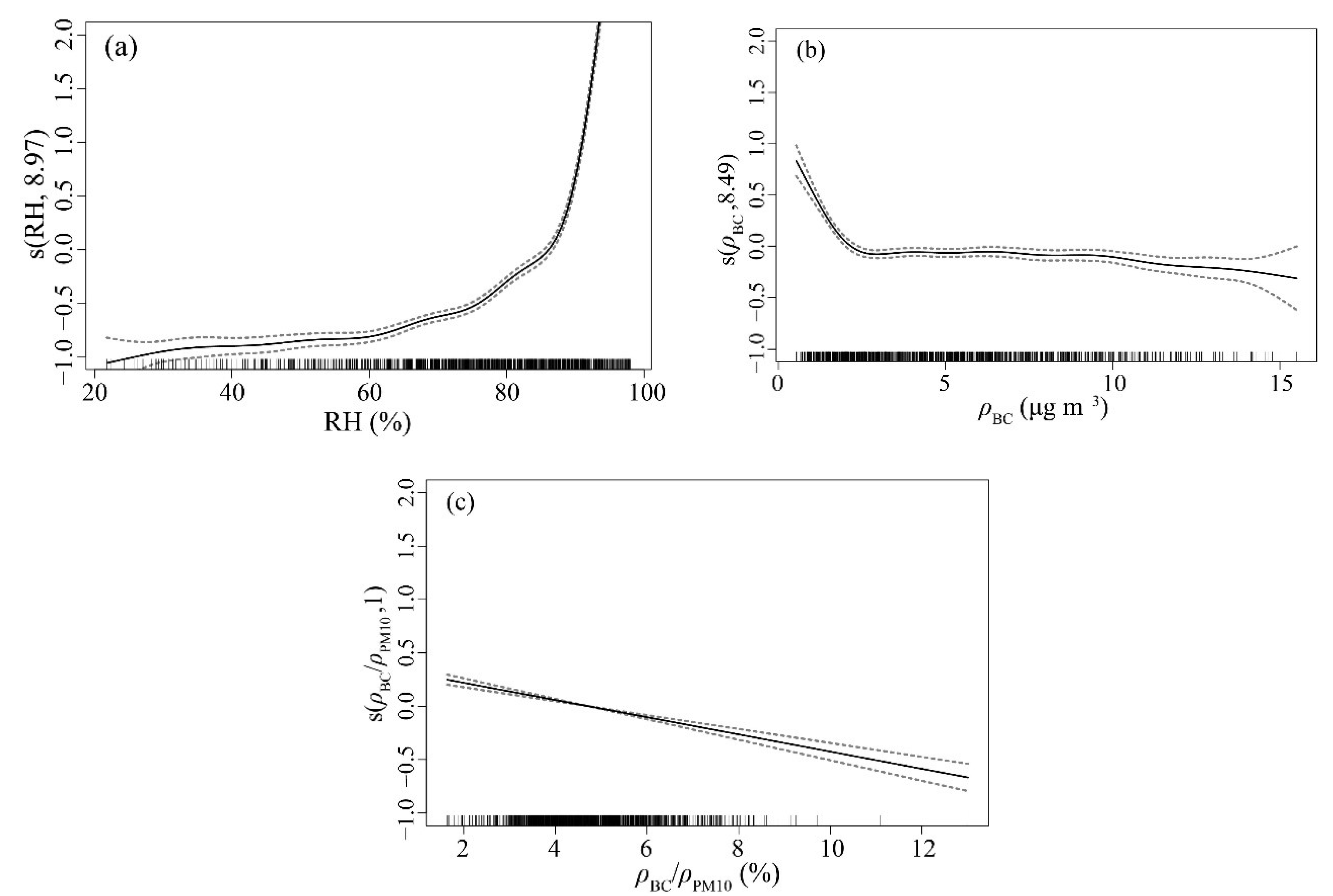
To further clarify the effect of BC on the hygroscopic growth of aerosol particles, aerosol scattering hygroscopic growth factor (
f) was selected as the response variable, RH,
ρBC and
ρBC/
ρPM10 were used as explanatory variables, and a GAMs model was established. It can be seen from the model results (
Table 5) that RH,
ρBC and
ρBC/
ρPM10 all passed the significance test of
α = 0.001. These three factors can well represent the growth factor of aerosol scattering hygroscopicity, of which RH has the greatest effect, followed by
ρBC/
ρPM10, and the smallest effect is from
ρBC. The R
2 and explained variance of the model are 0.72 and 89.5%, respectively, and the fitting effect of the model is good. The response graph for the influence of each covariate on
f is obtained and visually displayed in
Figure 7. In
Figure 7a,
f has a nonlinear positive correlation with RH. When RH > 80%,
f increases rapidly with the increase of RH. While in
Figure 7b,c,
f shows a decreasing trend with the increase of
ρBC and
ρBC/
ρPM10, which illustrates that the hygroscopic growth effect of aerosol particles is weakened, which is consistent with the research results of Zhang et al. [
54]. Aerosol hygroscopic growth caused by RH changes has the greatest influence on the aerosol extinction coefficient per unit of mass. When
ρBC/
ρPM10 increases,
f decreases. In addition, due to the non-hygroscopicity of BC [
53], the hygroscopic growth effect of aerosol particles is weakened, so the extinction coefficient per unit of mass of aerosol tends to decrease.
The occurrence of haze is closely related to high
ρPM2.5. According to the Environmental Air Quality Standard (GB3095-2012),
ρPM2.5 greater than 75 μg m
−3 is defined as PM
2.5 pollution concentration. Furthermore, the influence of environmental meteorological factors on the aerosol extinction coefficient per unit of mass under PM
2.5 pollution concentration is analyzed. According to Liu et al. [
55],
ρPM1~2.5/
ρPM10 increased significantly during haze episodes, while
ρPM1/
ρPM2.5 did not change obviously. Therefore, RH,
ρBC/
ρPM10,
ρPM1~2.5/
ρPM10 and
ρPM2.5/
ρPM10 are used to establish a multiple covariate model. The model results are shown in
Table 6. The four environmental meteorological factors have all passed the significance test of α = 0.01. The R
2 and explained variance of the model are 0.86 and 86.30%, respectively. At PM
2.5 pollution concentration, the sequence of the influence of covariates is as follows: RH >
ρPM1~2.5/
ρPM2.5 >
ρBC/
ρPM10 >
ρPM2.5/
ρPM10.
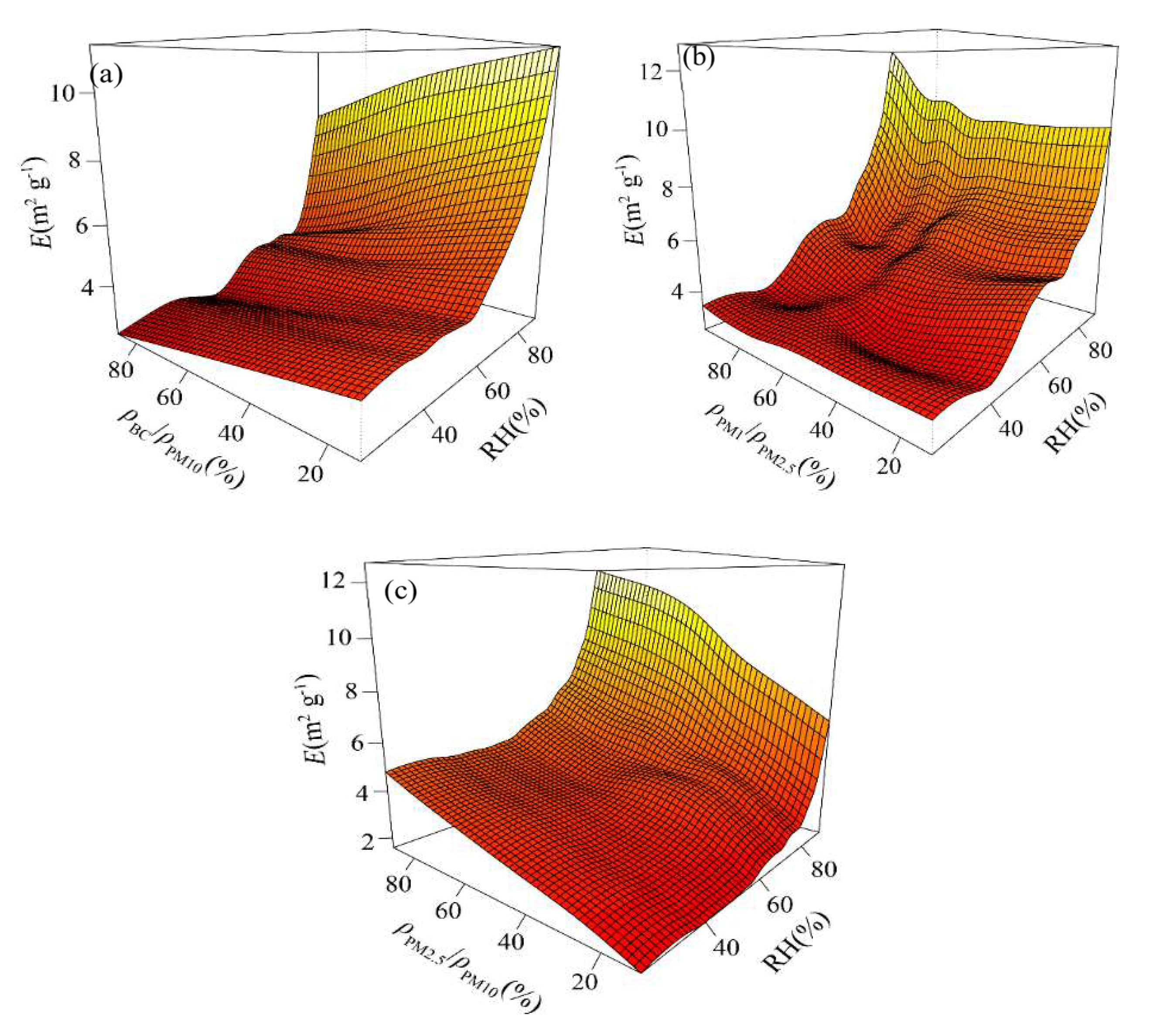
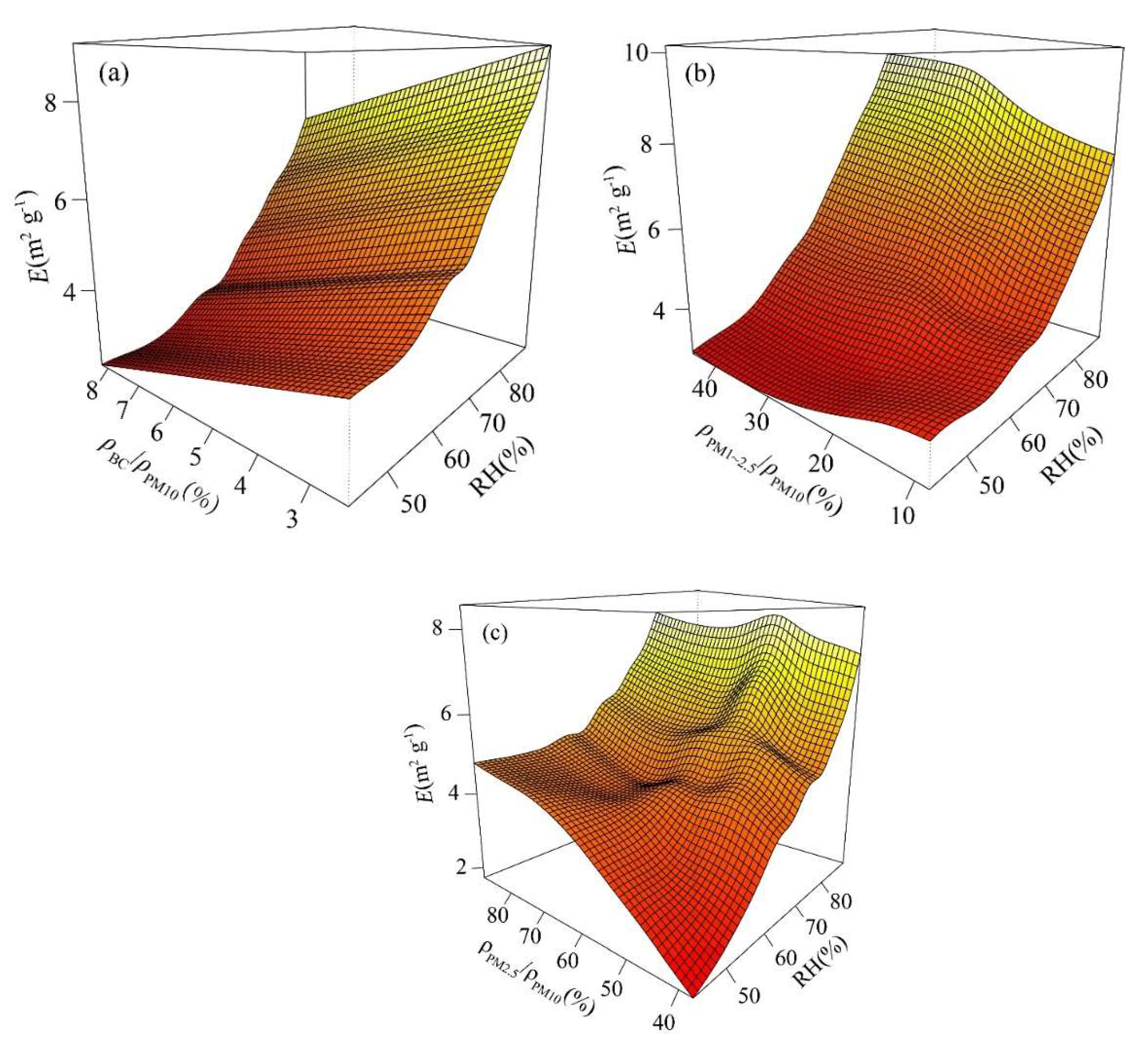
At PM
2.5 pollution concentration, the response graph for the influence of each covariate on the aerosol extinction coefficient per unit of mass is obtained and visually displayed in
Figure 8. The variation trend of the aerosol extinction coefficient per unit of mass with RH,
ρBC/
ρPM10 and
ρPM2.5/
ρPM10 is similar to that of the whole autumn and winter. The aerosol extinction coefficient per unit of mass increases with
ρPM1~2.5/
ρPM2.5, which is consistent with the results of Liu et al. [
55].


