
Vertical Eddy Diffusivity in the Tropical Cyclone Boundary Layer during Landfall

Shanghai Typhoon Institute, China Meteorological Administration, Shanghai 200030, China
Atmosphere 2022, 13(6), 982; https://doi.org/10.3390/atmos13060982
Submission received: 6 May 2022
/
Revised: 11 June 2022
/
Accepted: 14 June 2022
/
Published: 17 June 2022
(This article belongs to the Special Issue Atmospheric Boundary Layer Processes, Characteristics and Parameterization)
Abstract
:This study investigated surface layer turbulence characteristics and parameters using 20 Hz eddy covariance data collected from five heights with winds up to 42.27 m s−1 when Super Typhoon Maria (2018) made landfall. The dependence of these parameters including eddy diffusivities for momentum (Km) and heat (Kt), vertical mixing length (Lm), and strain rate (S) on wind speed (un), height, and radii was examined. The results show that momentum fluxes (τ), turbulent kinetic energy (TKE), and Km had a parabolic dependence on un at all five heights outside three times the RMW, the maximum of Km and S increased from the surface to a maximum value at a height of 50 m, and then decreased with greater heights. However, Km and S were nearly constant with wind and height within two to three times the RMW from the TC center before landfall. Our results also found the |τ|, TKE, and Km were larger than over oceanic areas at any given wind, and Km was about one to two orders of magnitude bigger than Kt. The turbulence characteristic and parameters’ change with height and radii from the TC center should be accounted for in sub-grid scale physical processes of momentum fluxes in numerical TC models.
1. Introduction
Turbulent mixing within the planetary boundary layer (PBL) of tropical cyclones (TCs) controls the radial and vertical distribution of momentum and enthalpy, consequently, changes the structure and intensity of TCs [1,2,3,4]. A better understanding of turbulent mixing would improve the accuracy of TC intensity forecasts [5]. Key parameters in PBL parameterizations are the eddy diffusivities of momentum (Km) and heat (Kt). These describe turbulent mixing and related fluxes in terms of the vertical gradient of the mean quantities, which control the feedbacks involving momentum, moisture, and heat between the surface and atmosphere. Numerical and observational studies have sought to constrain the turbulent mixing parameterizations in a numerical weather prediction (NWP) model for forecasting both TC track and intensification events over the ocean [6,7,8,9,10,11,12,13,14,15,16]. For example, Nolan et al. [17], Kepert [18], and Zhang et al. [19] found that improved estimations of the eddy diffusivity coefficient in the hurricane boundary layer are beneficial for hurricane prediction over the ocean. Gopalakrishnan et al. [20] reported that the value of Km controls the intensity of inflow in the boundary layer of TCs, and its parameterization leads to diverse solutions, based on analysis of dropwindsonde observations. More observations are required to improve simulations of hurricane or TC structure, path, and intensity.
Previous observation studies investigating the relationship between the vertical eddy diffusivities (VED) and wind speed (un) are limited to improving the turbulent mixing parameterization for TC forecasting. Based on aircraft observations during the Coupled Boundary Layer Air–Sea Transfer experiment [21], Zhang and Drennan [5] and Zhang et al. [18] estimated Km as a function of un at an altitude of 450–500 m over the ocean. Zhao et al. [22] identified a decreasing trend in Km values in high wind conditions (>40 m s−1) at heights of 500–670 m, using aircraft observations in five hurricanes. Katz and Zhu [23] used observational data to evaluate surface layer flux parameterizations. Based on flux tower observations, Tang et al. [24] concluded that Km values in a hurricane PBL are greater when the wind is blowing from inland than the ocean at un of up to ~30 m s−1 during typhoon landfall. Zhao et al. [25] analyzed mean wind profiles by a 350-m height flux tower during a typhoon landfall with un up to ~33 m s–1.
However, due to the difficulties in obtaining turbulence data during extreme typhoon conditions [24], previous studies have been mostly limited to low and moderate wind conditions, or in the PBL at >100 m height over the ocean [21,22,23]. Moreover, changes in surface conditions induce the boundary layer of TCs to differ significantly moving from the oceans to land [11,26]. The abrupt change in Km values at high wind conditions (>30 m s−1) has rarely been documented during hurricane landfall. In addition, the variations in Kt are unclear, especially at heights of <400 m during high-wind conditions [5]. In theoretical and numerical models, it is typically assumed that the value of Kt is equal to that of Km, or it is calculated using Prandtl and Schmidt numbers. However, Zhang and Drennan [5] found the Kt is much smaller than Km, based on ocean observational data obtained from the coupled boundary layer air–sea transfer hurricane experiment [26].
In order to fill the knowledge gap of the lower atmospheric boundary layer characteristics and the vertical profile of the VED at high wind conditions (>30 m s−1) in the inner-core region, this study focused on the turbulent mixing process with un up to severe typhoon category (42.27 m s−1) at heights of <200 m in the boundary layer during Super Typhoon Maria’s landfall, using high-frequency data (20 Hz) collected from multi-level flux observations on two flux towers. Although there remain difficulties in applying the method over tall, heterogeneous canopies, sloping surfaces, and as extreme typhoon conditions change rapidly making it difficult for an instrument and data system to survive [22,27], these data, after strict quality screening, are useful to constrain the key physical processes [28,29]. This paper is organized as follows: The data and processing methods are introduced in Section 2. Section 3 provides an analysis of the results and a comparison with previous studies. Finally, the conclusions and discussion for future research are presented in Section 4.
2. Material and Methods
2.1. Review of Typhoon Maria
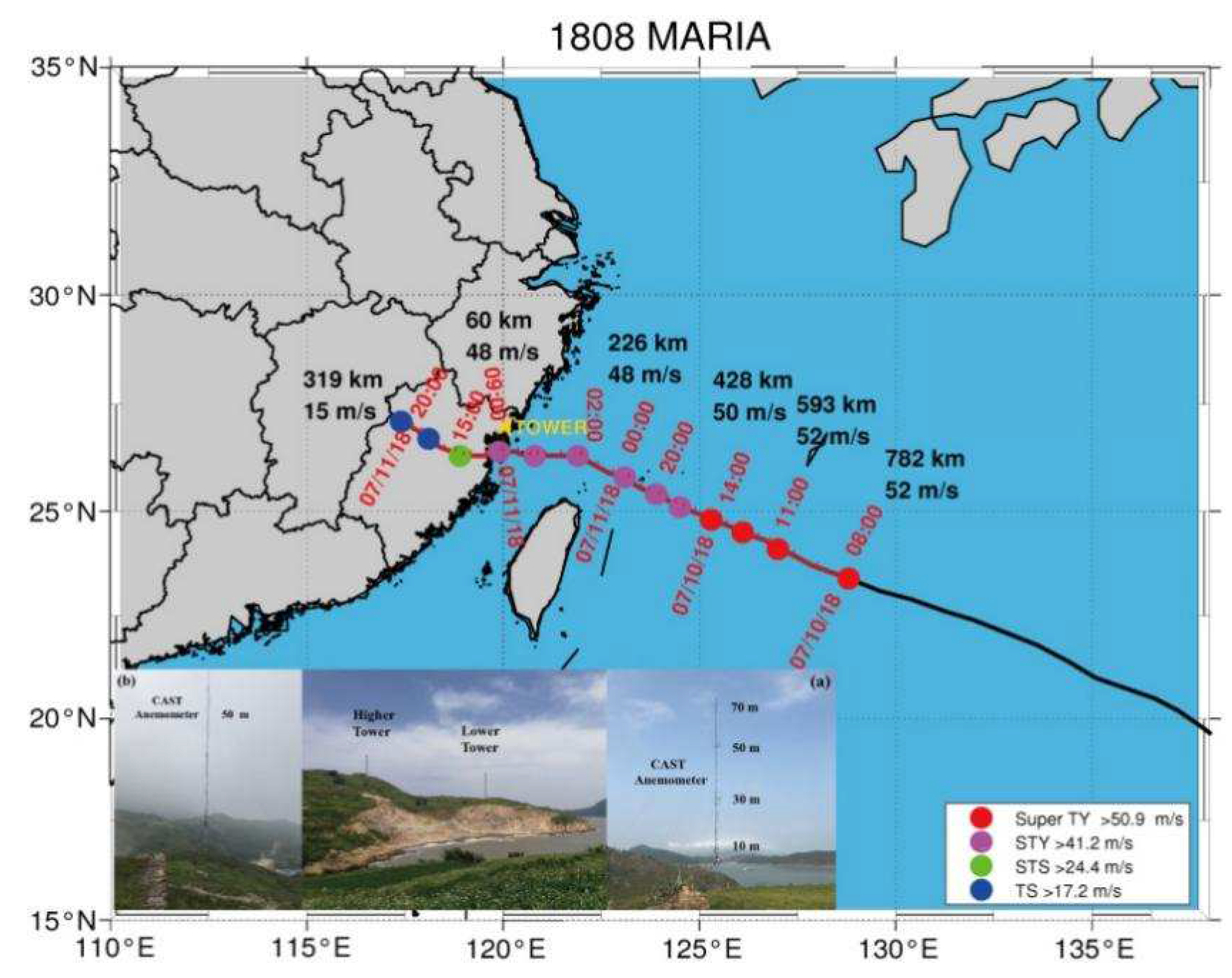
Super Typhoon Maria (2018) was the eighth typhoon to form in the Northwest Pacific Ocean in 2018. Figure 1 shows the track of the typhoon relative to the location of the two eddy covariance (EC) flux towers, and also the temporal changes in its track and intensity using data from the Shanghai Typhoon Institute of China Meteorological Administration (http://www.typhoon.org.cn/, accessed on 1 January 2022) [30]. After a short period of gradual intensification on 6 July, Typhoon Maria made landfall over Lianjiang County, Fujian Province, China, at 0850 local standard time (LST), 11 July 2018, when the maximum wind speed was ~38 m s−1. The location of landfall was ~68 km from the two observation towers. The towers at this time were located in the inner core region of the circulation, with the radius of maximum wind (RMW) at this time being ~60 km [31]. A maximum 10 min average un of 42.27 m s−1 was observed at 50 m height on the higher observation tower (110 m above the ground, or 170 m above sea level altitude (a.s.l)). After landfall, Typhoon Maria continued its track northward and weakened rapidly.
2.2. Observational Data and Analysis Method
The observation site was located on the coastline at Sansha, Fujian Province, China, and comprised two EC flux towers. The one meteorology tower (26°55′30″ N, 120°13′46″ E, 60 m above a.s.l.) was approximately 10 m from the coastline (Figure 1a) and is referred to as the low tower. The other meteorology tower (26°55′25″ N, 120°13′54″ E,120 m a.s.l.) was deployed at the top of the island (Figure 1b) and is referred to as the high tower. Each tower was equipped with four three-dimensional (3-D) ultrasonic anemometers (Campbell Scientific, Inc., Logan, UT, USA), with 1.5 m cantilever brackets at 10, 30, 50, and 70 m above the ground. The underlying surface of the two towers is grass that is <0.1 m in height. In this study, the data analyzed were collected from these two EC flux towers during the passage of Typhoon Maria (1808).
2.2.1. Eddy Covariance Method
The turbulent momentum flux τ (N m−2) was calculated using the direct eddy covariance (EC) method as follows:
where ρ (kg m−3) is the air density, and (m s−1), (m s−1), and (m s−1) are the along-wind (i), cross-wind (j), and vertical components of the wind fluctuations. The overbar indicates Reynolds averaging.
The turbulent kinetic energy (TKE) can be expressed as follows:
In the surface layer, the surface wind stress can be related to the surface frictional velocity u* by the standard K theory [32], and Km is usually parameterized as
where is the stability function that is calculated using the Monin–Obukhov length L and the following equation:
For the EC method, the Monin–Obukhov length scale is calculated as follows:
where is the mean temperature at the reference height z, g is gravitational acceleration, k is the von Karman constant, and is the flux of the virtual potential temperature at the observational height z.
The non-dimensional standard deviations of the three-dimensional wind velocity can be written as:
where α (= u, v, and w) denotes the longitudinal, lateral, and vertical velocity components, respectively, , and are the standard deviations () of u, v, and w, respectively.
Based on the standard K theory, the strain rate (S) and vertical mixing length (Lm) were estimated as follows:
where the overbar expresses the average over the length [33].
2.2.2. Data Processing and Quality Control
The data pre-processing mainly involved outlier removal, tilt correction, coordinate rotation corrections, and linear detrending [28]. Schmid et al. [33] proposed a method to examine the power spectra of turbulent fluctuations and this method was used in the present study, as follows.
- (1)
- Spikes in the datasets were removed using the criterion X(h) < (X − 4) or X(h) > (X + 4), where X(h) denotes the original data, X is the mean over the averaging interval, and is the standard deviation [34].
- (2)
- The calculation of VED was omitted when the corresponding u* was < 0.01 m s−1. No gap filling was used.
- (3)
- Based on the coastline features near the measurement site, the onshore wind direction varied from 52.5° to 227.5°, and the offshore wind direction varied from 272.5° to 5°. The wind data from the back of the three-dimensional sonic anemometer measurements of the lower tower (249–269°) and higher tower (68–88°) were removed due to the turbulent eddies generated by the towers.
- (4)
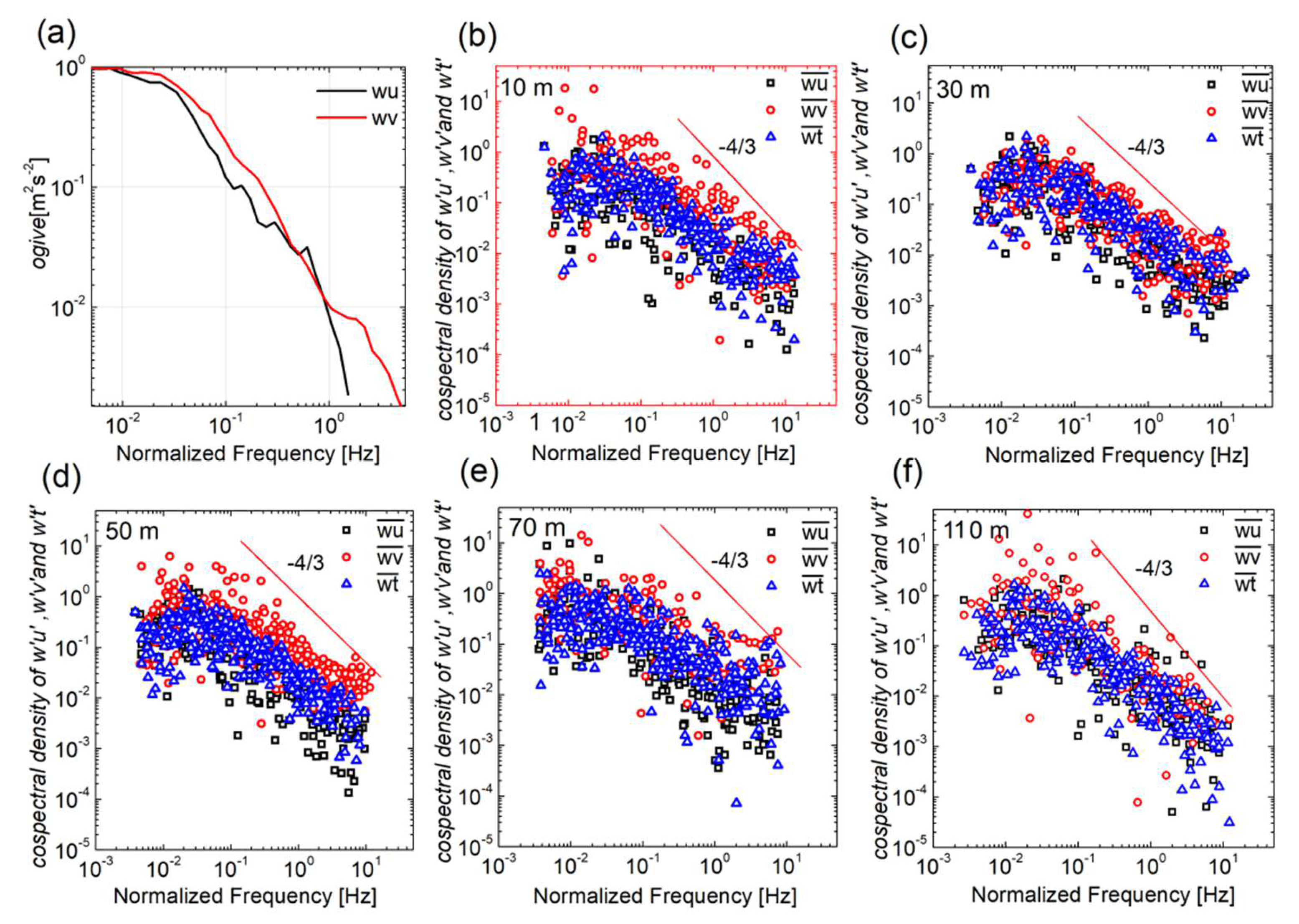
- Averaging period: A cumulative frequency curve (ogive) can be used to understand the turbulent stationarity and its spatial scale, which is then typically used to determine the appropriate time period required to calculate the turbulent flux [34].where x (= u, v, and T) denotes the along-wind (u) and cross-wind (v) components, and ultrasonic virtual temperature (T), respectively, is the cospectrum of w’u’, w’v’, and w’T’ at frequency . As we can see, for the ogive curves of w′u′, w′v′, and w′T′ shown in Figure 2a, the ogive curves of the w′u′, w′v′, and w′T′ approached a constant value at an averaging period of 5 min when it converged towards 0.005 Hz. Therefore, an averaging period more than 5 min is suitable for calculating the turbulent flux and can represent the total flux. Hence, we chose 10 min for the averaging period to calculate the moment and heat flux.
- (5)
- A turbulence (co)spectrum check.
According to the Kolmogorov theory for the inertial subrange [35], a turbulence (co)spectrum of the slope check has been used for turbulence data quality control in previous studies, such as Zhang et al. [10,11], Fortuniak et al. [36], Zhao et al. [21], and the one-dimensional spectrum , of any wind component, , normalized by the squared friction velocity , can be expressed in the form
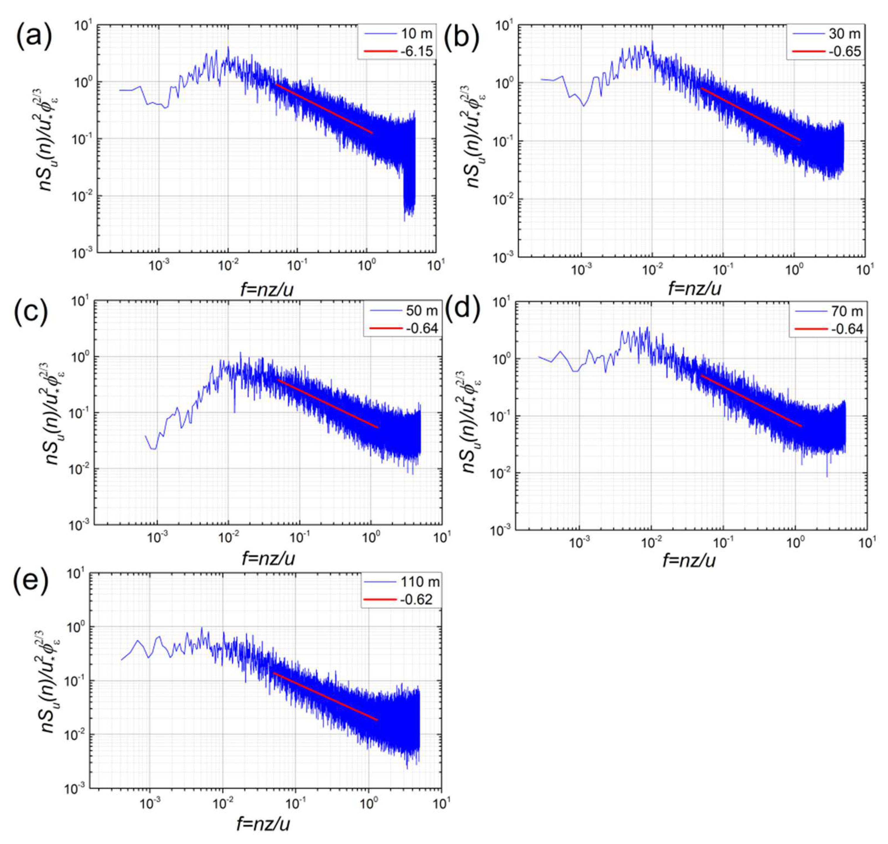
where n is the natural frequency, f is the non-dimensional frequency, are universal Kolmogorov inertial subrange constants and κ is the von Kármán constant, is the non-dimensional dissipation rate of TKE (ε). The is a function of the stability parameter, , where L is the Obukhov length. The velocity spectra normalized by and , are presented in Figure 3. Our neutral limits from the stable side included the spectra from the narrow stability band 0 < ζ < 1.2 (similarly, in the unstable limit) as compared to the relatively wide band (0 < ζ < 0.1) used by Kaimal et al. [37]. In the inertial subrange, the spectra slopes of the horizontal wind speed (u) ranged from −0.61 to −0.65; they follow the −2/3 slope quite well.
Cospectra analyses of the measured turbulent fluctuations are a useful tool for testing the reliability of flux data. Figure 2b–f shows examples of cospectra of the longitudinal (u), lateral (v), and ultrasonic virtual temperature (T) averaged from data collected at five heights over three days during the landfall of Typhoon Maria. Previous studies indicated that the empirical cospectra are not as well formed as the empirical spectral functions [36]. So positive values of for 0.1 < f < 5 were used to fit the power function to the cospectrum in the inertial subrange, and the −4/3 line is plotted by green line in each panel for the convenience of comparison with the ideal situation. In the inertial sub-range, the cospectra slopeon for the difference is that the vertical turbulent compons of the horizontal wind speed (u, v) and T ranged from 0.78 to 1.29, and a majority of the three cospectra was close to the ideal slope of –4/3, especially for the longitudinal wind components. The sharp of the three cospectra trends rolled-off at f = 0.01 Hz at each height. However, the slopes deviated from the –4/3 slope more obviously with height. In addition, some low-frequency and high-frequency data deviated from the –4/3 slope on a log-log scale (Figure 2). Ortiz-Suslow et al. [38] and Dorman et al. [39] found that there may be natural deviations in the inertial subrange bandwidth and spectral slope from Kolmogorov’s turbulence that occur within ±20% caused by mechanical wind–wave interactions. Compared with the classical 4/3 ratio in the inertial subrange at a homogenous flat surface reported by Kaimal et al. [37] for the Kansas experiment, the sensor noise rising at the high-frequency may be due to the high wind and high wet environment of the typhoon. It may also generate larger-scale eddies during typhoon landfall due to the effect of flow field shear on the turbulence spectrum in the coast process [39].
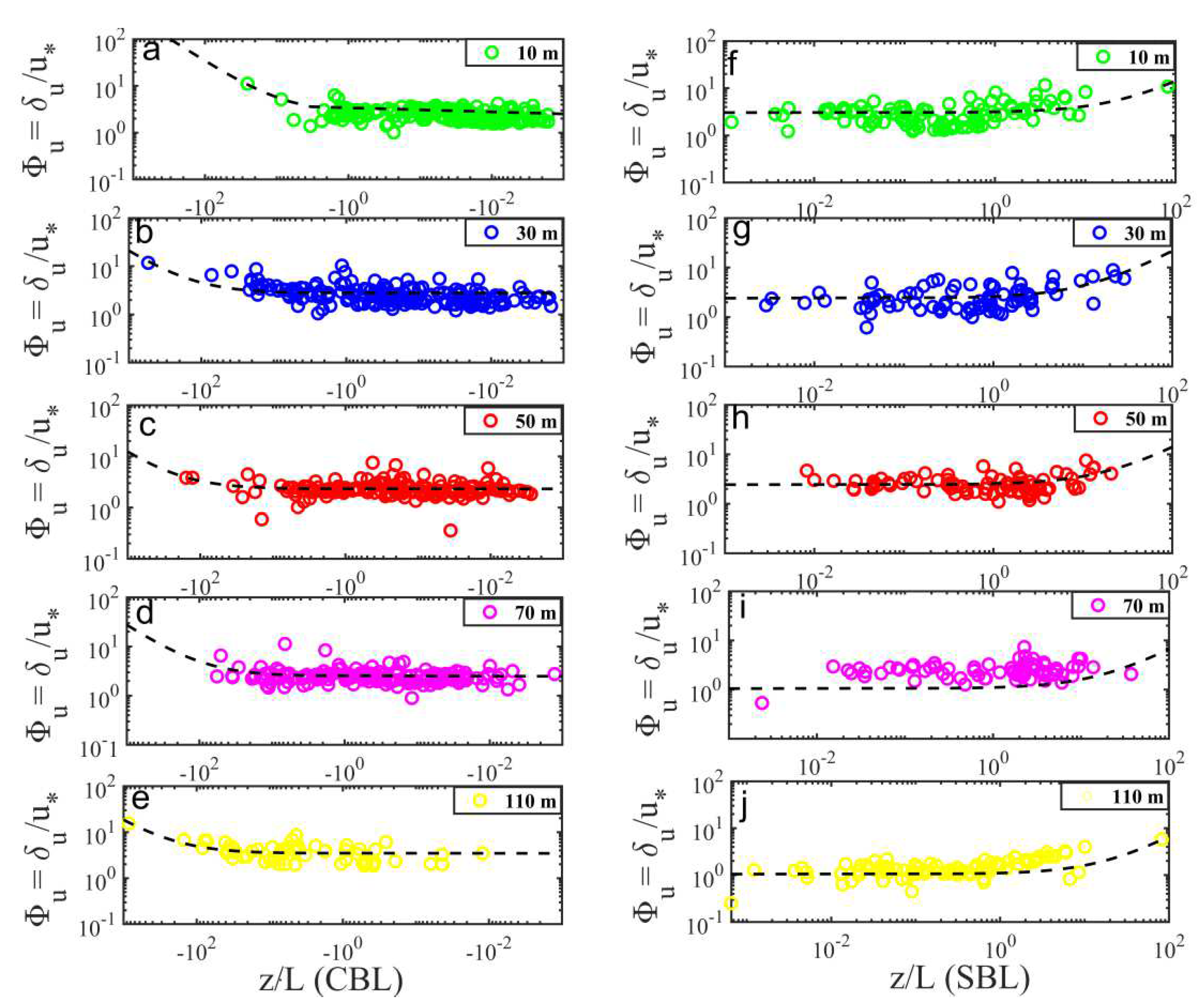
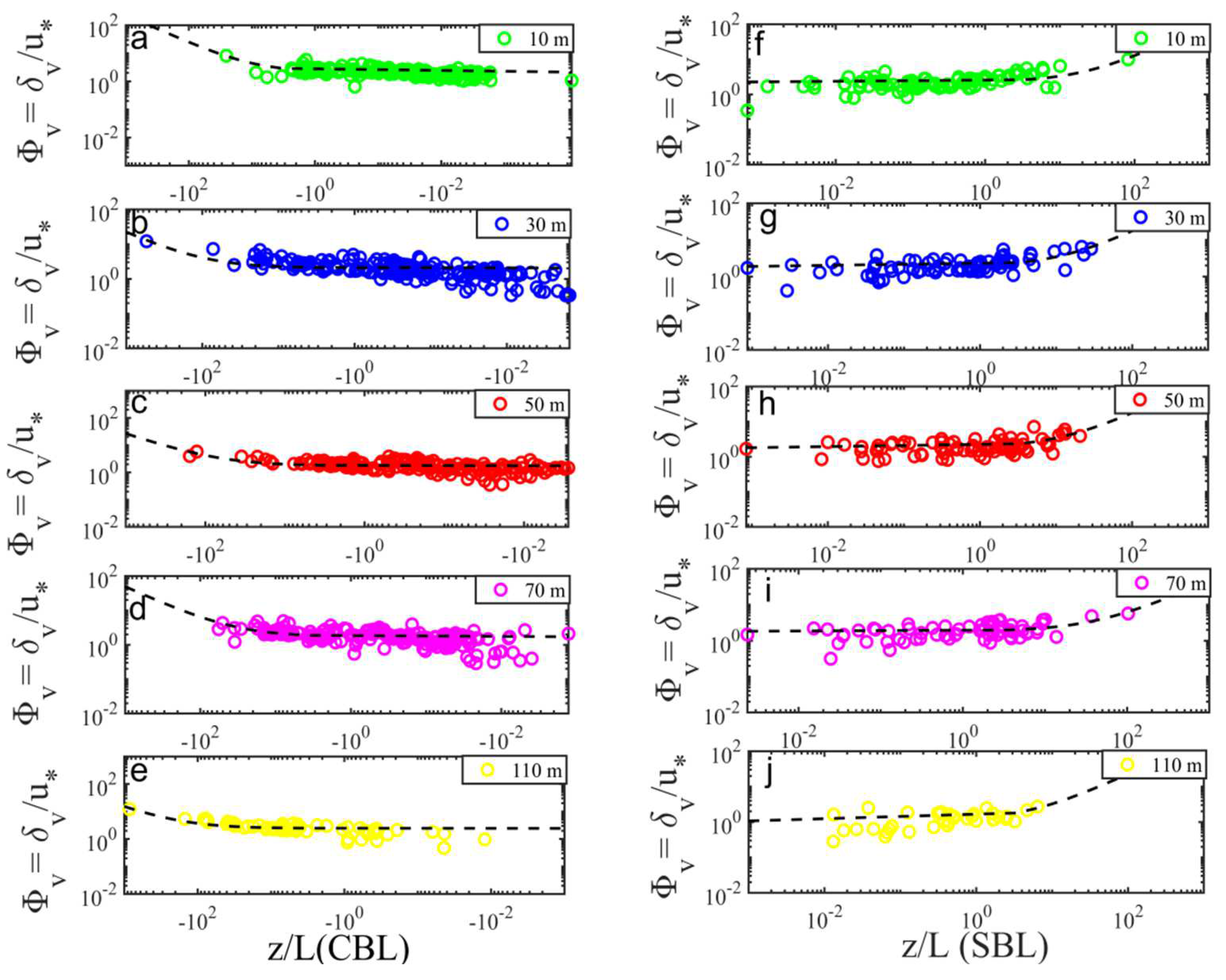
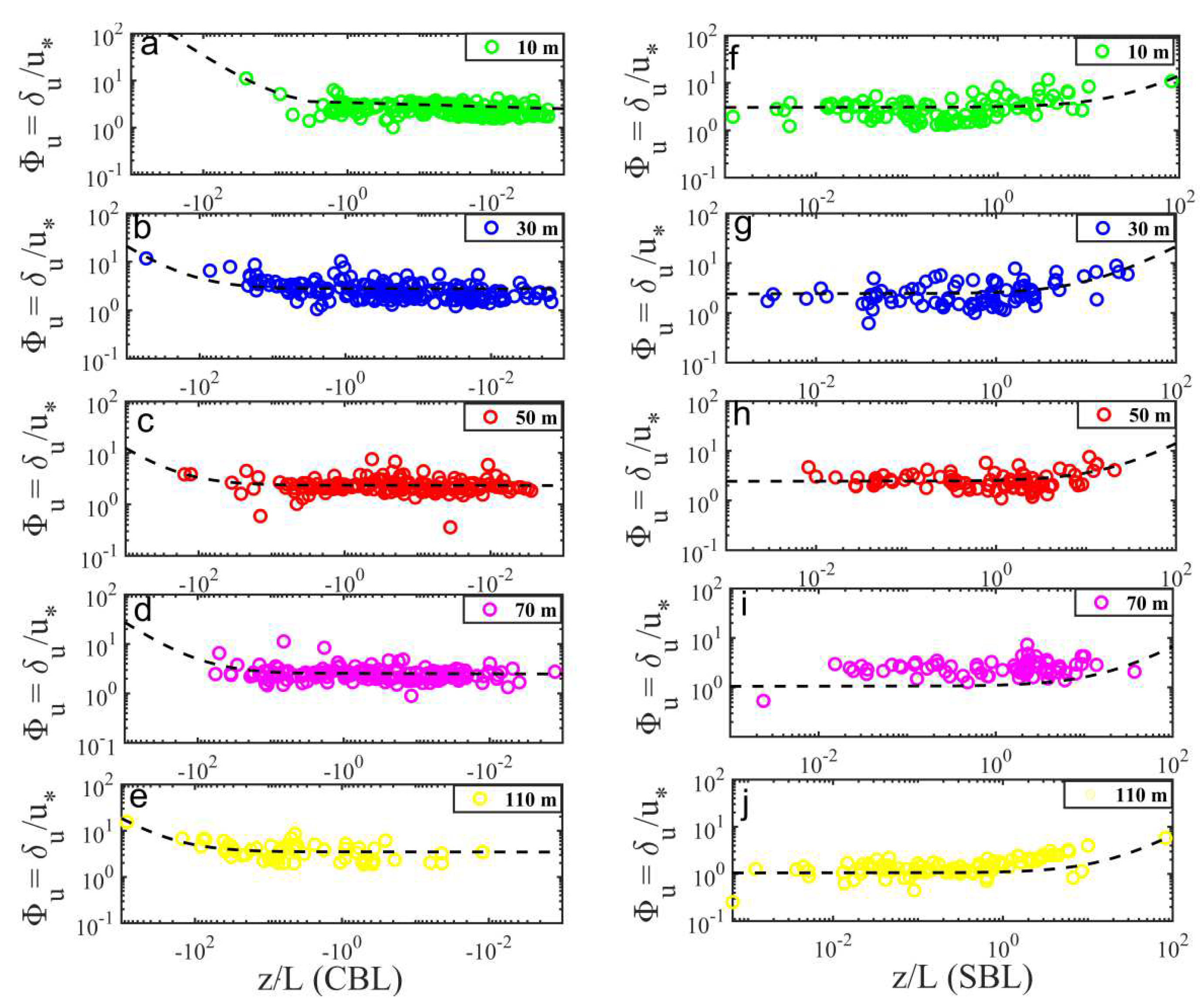
Verification of the Monin–Obukhov Similarity (MOST) during typhoon landfall: The variations in the normalized standard deviations of turbulence with the dimensionless stability parameter () have been widely used to evaluate the applicability of the MOST in a series of previous studies [34,35]. According to MOST, any scaled statistics of turbulence at reference height z are universal functions of the dimensionless stability parameter, z is the observation height and L is the Obukhov length scale (see Equation (6)).
Figure 4, Figure 5 and Figure 6 show plots of the , , and versus with the left panels (Figure 4, Figure 5 and Figure 6a–e) representing unstable (z/L < 0) conditions and the right panels (Figure 4, Figure 5 and Figure 6f–j) representing stable ( > 0) conditions at five heights during Typhoon Maria’s landfall. The blank dashed lines are exponential fitting lines correspond to . Note that, irrespective of whether the conditions were stable or unstable, , , and exhibited an obvious relationship with , and this is consistent with classical Monin–Obukhov z-less scaling [35]. It is evident that the data collected in the coastal region during the typhoon period were generally in agreement with previous studies that follow the canonical MOST predictions during the non-typhoon period [40,41]. From the perspective of stability, the exponential fitting lines of unstable layers and stable layers were consistent with the –1/3 power law, whereas the formation of stable layers followed the polynomial fitting law from observations at the Downs site. However, our observations during the typhoon period showed a larger scatter of individual data points as compared with the results measured from the North Carolina coastal zone [40]. Additionally, showed somewhat greater scatter than . The larger scatter of data and poor correspondence of with the classical MOST theory may possibly be related to non-local mixing in the complexity of the coastal terrain and typhoon conditions; the shear production rate exceeded the buoyant production rate in the high wind condition. The heights of 10 and 110 m exhibited the smallest and greatest deviation from the MOST theory, respectively.
3. Results and Discussion
3.1. General Meteorological Conditions
3.1.1. Wind Characteristics during the Observation Period
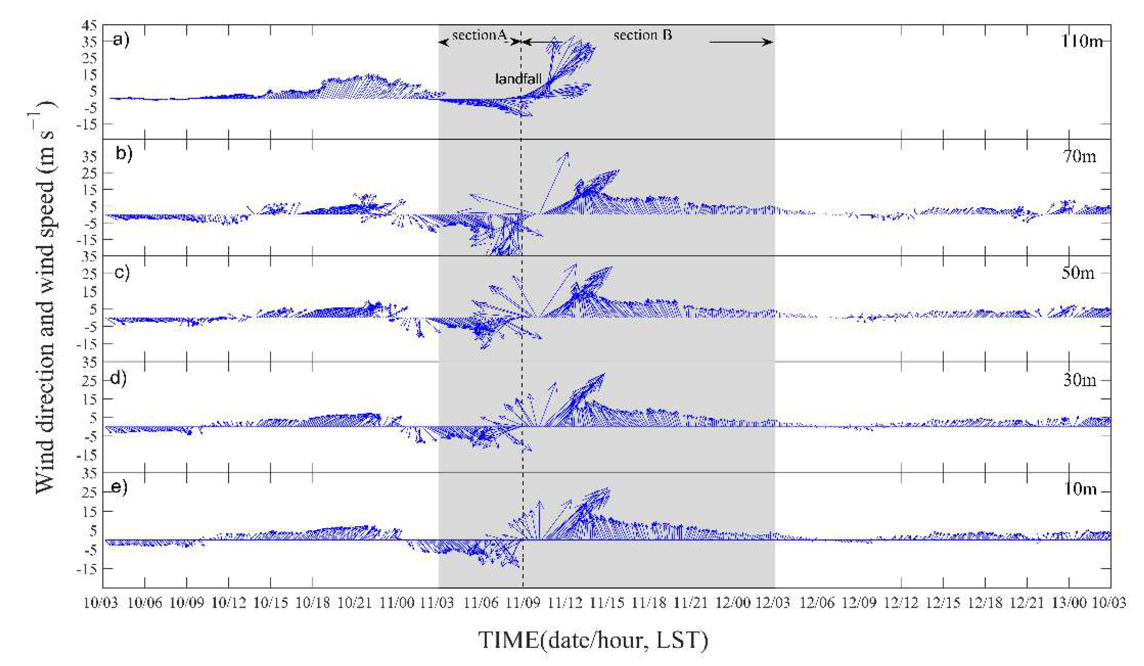
Figure 7 shows 10-min averaged wind directions and speeds from the five heights during Typhoon Maria’s landfall. Unfortunately, due to the lack of measurement data from the high tower, there was no wind information from a height of 110 m after landfall. It still can be seen that the wind directions at the five heights exhibited a significant daily cycle from northwest in the daytime (offshore) to northeast in the nighttime (onshore) related to the land–sea breeze. In addition, the wind direction at a height of 110 m on the high tower was slightly different from that of the low tower, which is likely due to the topography. For the wind speeds, compared with the annual 10-min mean un of 5–10 m s−1, a maximum 10-min mean un of 42.27 m s−1 was observed in the front right quadrant of the typhoon at a height of 110 m on the high tower as Typhoon Maria passed through the towers. The un became higher and peaked before and after the typhoon passed. With increasing height, the first peaks from the offshore wind direction before the typhoon passed had a un of 16.57, 19.05, 22.26, 29.61, and 21.28 m s−1. The second peaks from the onshore wind direction after the typhoon passed had a un of 36.51, 36.79, 39.06, 39.67, and 42.27 m s−1 (Table 1). In addition, the offshore wind direction changed from approximately southeasterly to southwesterly at the first peak, and from approximately southeasterly to southwesterly during the second peak. This made it possible to conduct wind-direction-dependent analysis of the wind characteristics of this strong typhoon.
3.1.2. Meteorological Conditions
To better depict the meteorological conditions during the observation period, Figure 8a shows a time-series of the 10-min averaged TKE values, 1-h averaged air pressure from the Sansha meteorological observatory (located near the EC flux towers), precipitation during landfall (Figure 8b), distance from the typhoon center to the tower during the period 0000 LST 10 July to 0000 LST 12 July, and radar reflectivities (dBz) at Z = 2 km from 0200 to 1200 LST 11 July 2018 obtained by the Ningde weather radar before and after landfall of Typhoon Maria.
Section A is the period prior to typhoon landfall and section B is the period after typhoon landfall. Typhoon Maria passed over the observation towers at about 0850 LST 11 July 2018 (Figure 8c). The smallest distance between the observation towers and the center of Typhoon Maria was about the RMW (60 km: Figure 8c). The 10-min averaged TKE on the lower tower increased as Typhoon Maria approached and reached a maximum value of 102.6 m2 s−2 at a 50 m height on the lower tower ahead of landfall, and then decreased rapidly. This may indicate that the inner core of the typhoon increased the local values of the TKE. The 10-min averaged TKE on the high tower exhibited an opposite trend from 0600 to 0800 LST 11 July 2018 before landfall, and the 1-h averaged TKE on the high tower was smaller than on the lower tower during the 3 h (from 0600 to 0800 LST 11 July) (Figure 8a). The main reason for the difference is that the vertical turbulent component decreased abruptly during this 3 h. It is possible that the momentum transport was weak during the period, and the momentum fluxes (τ) were highly correlated with the TKE. This also implies that the momentum transport was closely related to the turbulent intensity. The air pressure at the Sansha meteorological observatory, which is ~1 km from the towers, began to decrease as Typhoon Maria approached, and the air pressure dropped to its lowest value (968 hPa) at this time when the minimum distance between the towers and typhoon center was ~60 km at 0800 LST 11 July 2018.
3.2. Variations in Momentum Fluxes and Turbulent Kinetic Energy with wind Speed at Each Height
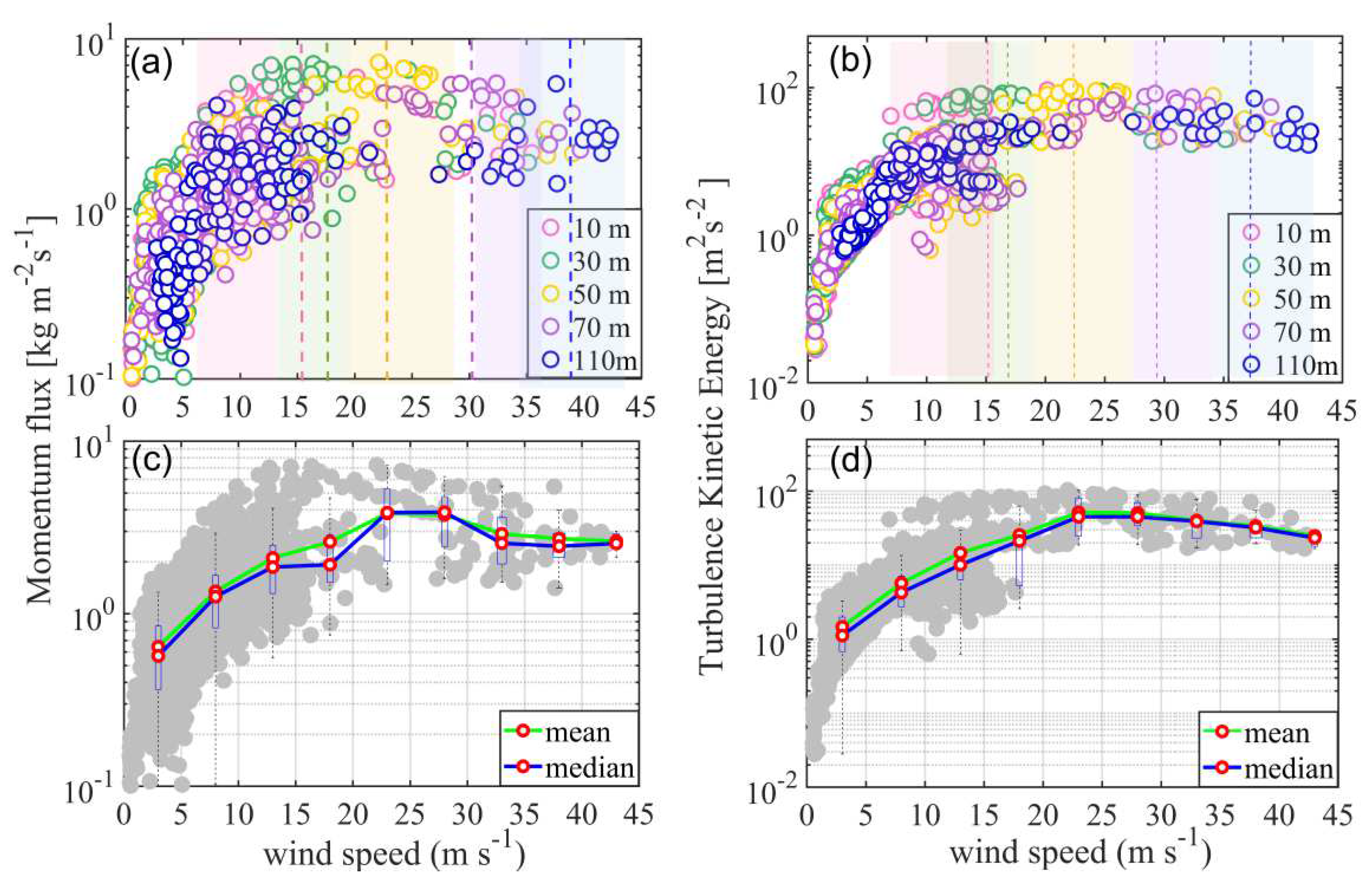
Momentum fluxes obtained by the EC method are plotted as a function of un at the five measurement levels (10, 30, 50, 70, and 110 m) on the two towers during Typhoon Maria (Figure 9a). |τ| values at all heights exhibited a clear parabolic trend with un, and at low-moderate un (<30 m s−1), |τ| initially increased up to 22 m s−1, at which point |τ| was 11 m−1 s−2, then slowly decreased with un increasing further (>30 m s−1). Moreover, the values of |τ| in the un range of 15–30 m s−1 was higher than previous observational results from oceanic and inland regions [19,22]. For example, |τ| obtained in this study was five times larger than that at sea at heights of 420–500 m obtained using aircraft observations [22]. Previous studies have mostly attributed this to surface roughness over an island, which is greater than that over the open ocean [22].
At higher wind speeds (>30 m s−1), |τ| decreased with increasing un, this phenomenon is similar to results from some previous studies, which found that |τ| or TKE no longer increase significantly at high wind speed [38,39,40]. However, this result is inconsistent with the previous observational study by Zhao et al. [42], who found |τ| increased with increasing un to 60 m s−1 over the ocean.
Furthermore, |τ| peak values varied with height. With increasing height, |τ| peaked at 24.1, 39.0, 40.6, 24.2, and 20.5 m−1 s−2, and the corresponding un at the |τ| peaks were 12.5, 14.6, 22.1, 32.4, and 37.6 m s−1, respectively. The maximum |τ| value occurred at 50 m height (40.6 m−1 s−2), and then decreased with height above 50 m.
The variations in TKE against un at the five measurement levels are shown in Figure 9b. In general, the TKE varied similarly to the momentum flux, because the TKE is generated by wind turbulence and the momentum flux is generated from the wind flow. As such, the TKE was highly correlated with |τ| as shown by Equations (1) and (2). The TKE increased significantly at low and moderate wind speeds (<22 m s−1) and slightly decreased at higher wind speeds. In addition, the maximum TKE values also varied with height. With increasing height, the TKE peaked at 24.1, 39.0, 40.6, 24.2, and 20.5 m−2 s−2, and the corresponding un values at the TKE peaks were 10.0, 16.7, 22.3, 28.6, and 38.0 m s−1, respectively. The maximum TKE peaked at 50 m height with a value of ~100 m2 s−2. The result showed that the TKE and |τ| peaks increased with height from 10 to 50 m, and then decreased at greater heights with the corresponding wind speeds increasing continue.
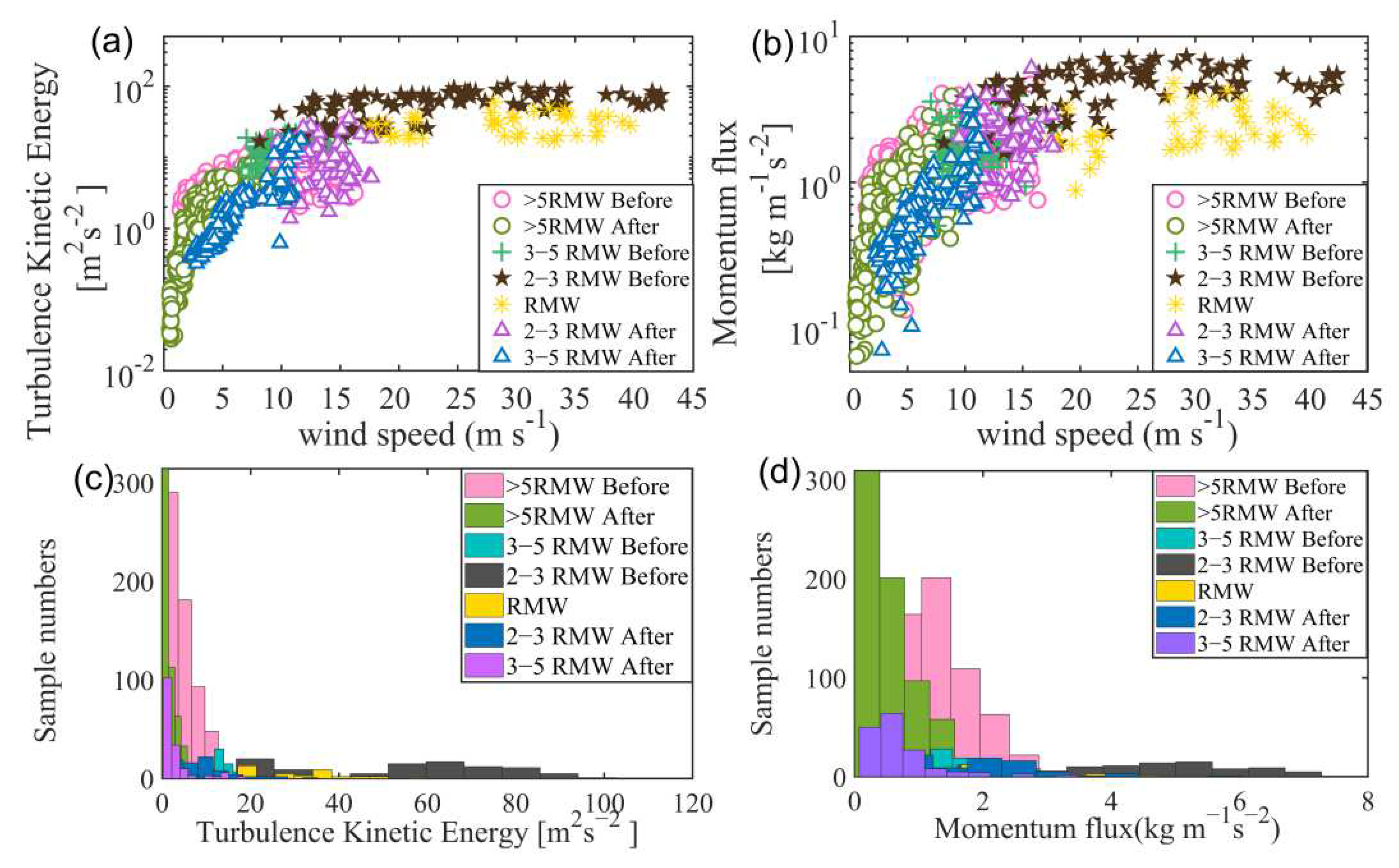
3.3. Variations in Momentum Fluxes and Turbulent Kinetic Energy with Distance from TC Center
Although both |τ| and TKE exhibited parabolic trends with increasing un at all five heights (Figure 9c,d), these relationships changed with distance from the TC center. The |τ| and TKE variations with un are plotted as a function of the distance to the TC center normalized by the RMW in Figure 10a,b. All data were classified into seven categories according to the TC radius normalized to the RMW. The first and second categories are at distance outside five times the RMW(5 RMW) from the TC center before and after typhoon landfall, respectively; The third and fourth categories are from the region between the three and five times RMW (3–5 RMW) before and after typhoon landfall, respectively; The fifth and sixth categories are from the region between the two and three times RMW (2–3 RMW) before and after typhoon landfall, respectively; the seventh category is from the region near the RMW. At larger radii (outside 3 times RMW), both |τ| and TKE increased significantly with increasing un at <15 m s−1. With the approach of the typhoon (within three times RMW), both |τ| and TKE increased slowly with increasing un. Most of |τ| and TKE data were concentrated in the region of two to three times the RMW before the typhoon landfall, and the |τ| and TKE values were 60 m−1 s−2 and 10 m−2 s−2, respectively, which were five to ten times larger than that in the 2–3 RMW region after typhoon landfall. In the case of the TKE, when the un was >15 m s−1 in the region of 2–3 RMW before typhoon landfall, the TKE values no longer changed significantly as the un further increased. This shows that the TKE was basically constant with height in the 2–3 RMW region before the typhoon landfall, due to adequate vertical turbulent mixing in the surface layer. The constant of TKE with height may reflect that the constant surface layer exists in the 2–3 RMW region before the typhoon landfall. Near the eyewall region at high wind speeds, the |τ| and TKE values decreased slightly with increasing un. The values were smaller than those in the region of 2–3 RMW prior to typhoon landing at similar wind speeds, whereas five times higher than those in the outer typhoon core regions.
3.4. Vertical Diffusion Transport of Momentum
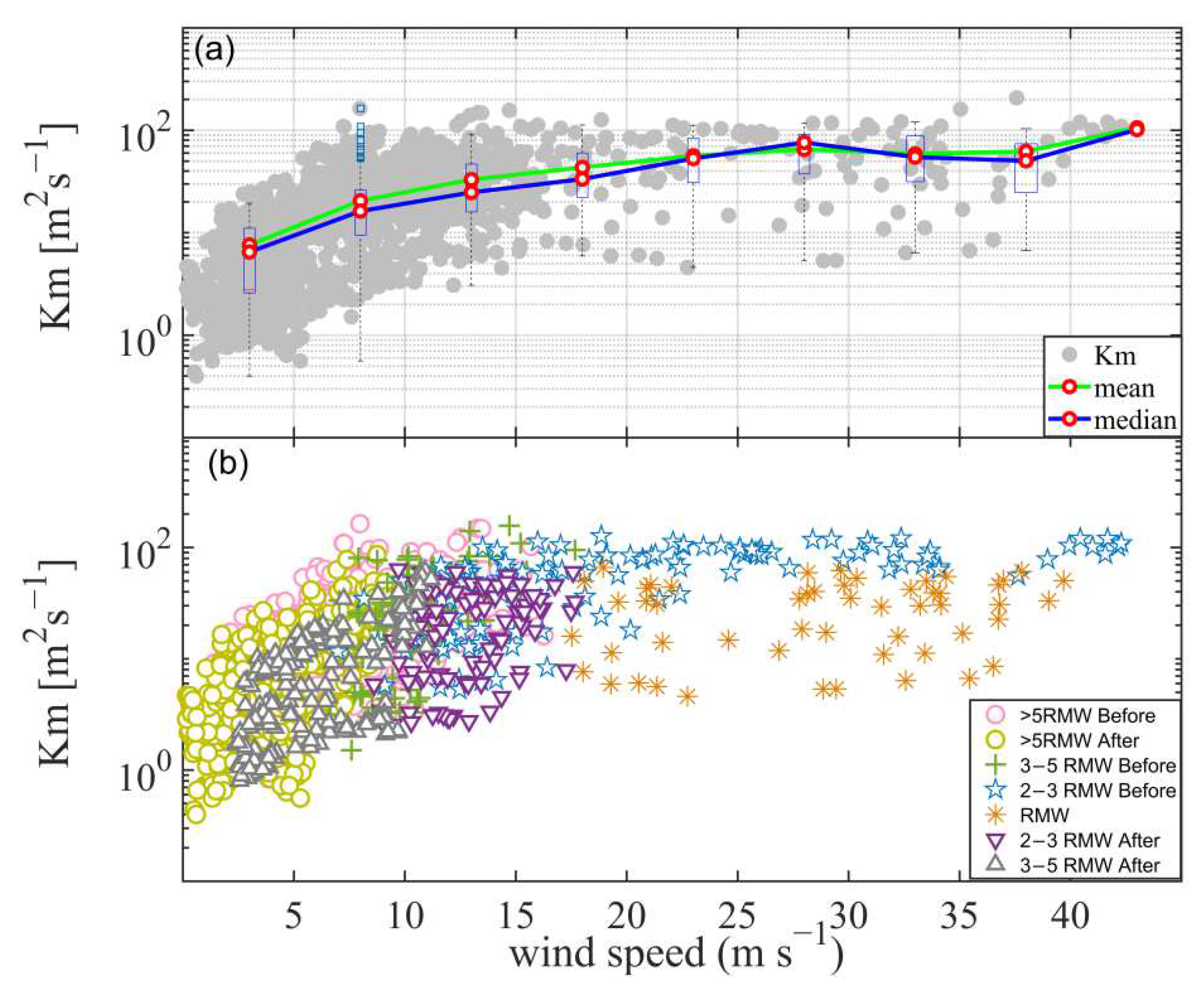
Figure 11a shows the bin-averaged Km values estimated using the eddy covariance method as a function of un at all levels during landfall of Typhoon Maria. Seven wind speed bins of 5 m s−1 were chosen, ranging up to 45 m s−1.
It was expected that Km would increase gradually with increasing un at <30 m s−1, and then decrease slightly with un up to 40 m s−1. Km increased again when the un was >40 m s−1, but at a lower increasing rate than at < 30 m s−1. The spatial patterns and magnitude of the coastal variations in Km values with un are similar to the aircraft observation results of Zhao et al. [22]. The slope of increasing Km with un at <30 m s−1 is similar to the results of Zhang and Drenman [5], Tang et al. [24], and Zhao et al. [25]. The decreasing Km at wind speeds of >30 m s−1 is different from the observational results of hurricane eyewalls at 500 m altitude from Zhang et al. [19], which shows that Km consistently increases with increasing un to >40 m s−1. The coastal Km values obtained in the present study reached uniform values at a slower un (28 m s−1) than in the studies of Zhang et al. [19] and Zhao et al. [22] over oceanic regions and Tang et al. [24] over inland areas. This may be due to the larger momentum flux and lower altitude of the present study conditions. The presented observational data support the findings of Zhang and Zhu [11] and suggest that different boundary layer parameterizations should be used for vertical eddy diffusivity over land and oceanic regions in TC simulations and forecasts.
Km values tended to increase with un outside three RMW, but were less dependent on un near the eyewall region (Figure 11b). The higher values of Km were concentrated in the region of 2–3 RMW before typhoon landfall, with an almost constant (100 m−2 s−1) high wind speed of 20.0–42.5 m s−1. This indicates that the bulk parameters should be different over different regions when modeling the typhoon PBL.
3.5. Vertical Eddy Diffusivity of the Sensible Heat Flux
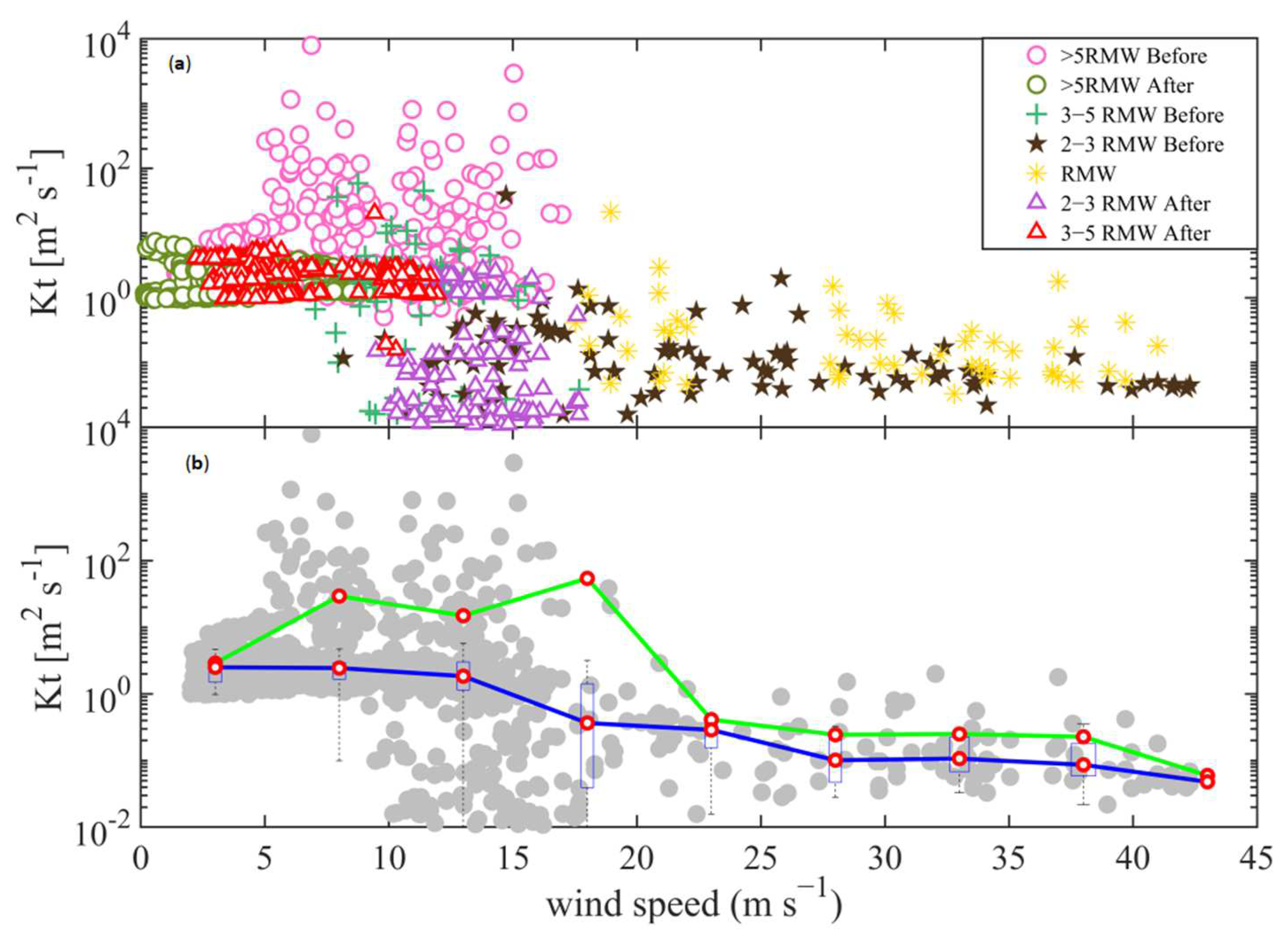
Figure 12a shows the bin-averaged Kt values estimated by the EC method as a function of un at the five height levels during the landfall of Typhoon Maria. The different colored symbols represent different regions of Typhoon Maria (Figure 12b).
In general, Kt decreased with increasing mean un from 5 to 45 m s−1, and most of Kt following the trend were from the region before typhoon landfall. The decreasing trend was opposite to the trend for Km at moderate un. Most Kt values were <100 m2 s−1, with a small number of large values of Kt (>100 m2 s−1) in the region outside 5 RMW before typhoon landfall (Figure 12b). From the median line of Kt, all values of Kt were <12 m2 s−1 (Figure 12a). Kt was about one to two orders of magnitude smaller than Km, possibly because large and small eddies usually transport the sensible heat flux in opposite directions.
The variations in Kt with un were different between outside 3 RMW and 1–3 RMW. Kt values showed a clear decrease with increasing wind speed located in the 1–3 RMW, but Kt exhibited little dependence on un outside 3 RMW (Figure 12b). Kt from the region outside 3 RMW was 10 times larger than that from the inner core region.
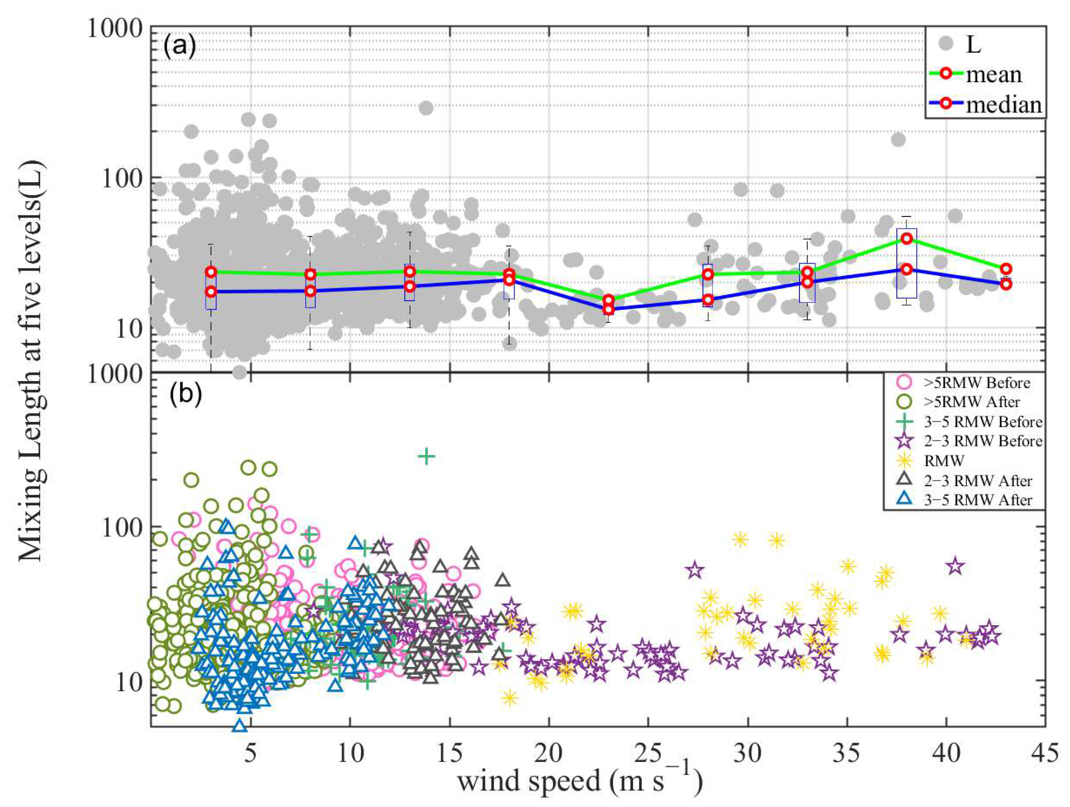
3.6. Variation in Vertical Mixing Length
Lm in models needs to be parameterized by observations [20], and it can be directly estimated from the eddy covariance data using Equation (8). The relationship between Lm and un exhibited segmented trends (Figure 13a). At weak and moderate wind speeds (<20 m s−1), there was a weak dependence of Lm on wind speed at each level, due to a large scatter during weak winds outside 5 RMW (Figure 13b). It is consistent with the result of Tang et al. [24], who showed a weak dependence of Lm on the wind speed over land and Zhang et al. [19] using aircraft observations over the ocean. While, at high wind speeds (>30 m s−1) in the region of 1–3 RMW before typhoon landfall, Lm increased with un and then began to decrease at >38 m s−1. This indicates that a single PBL scheme with a constant mixing length is inappropriate for hurricane conditions.
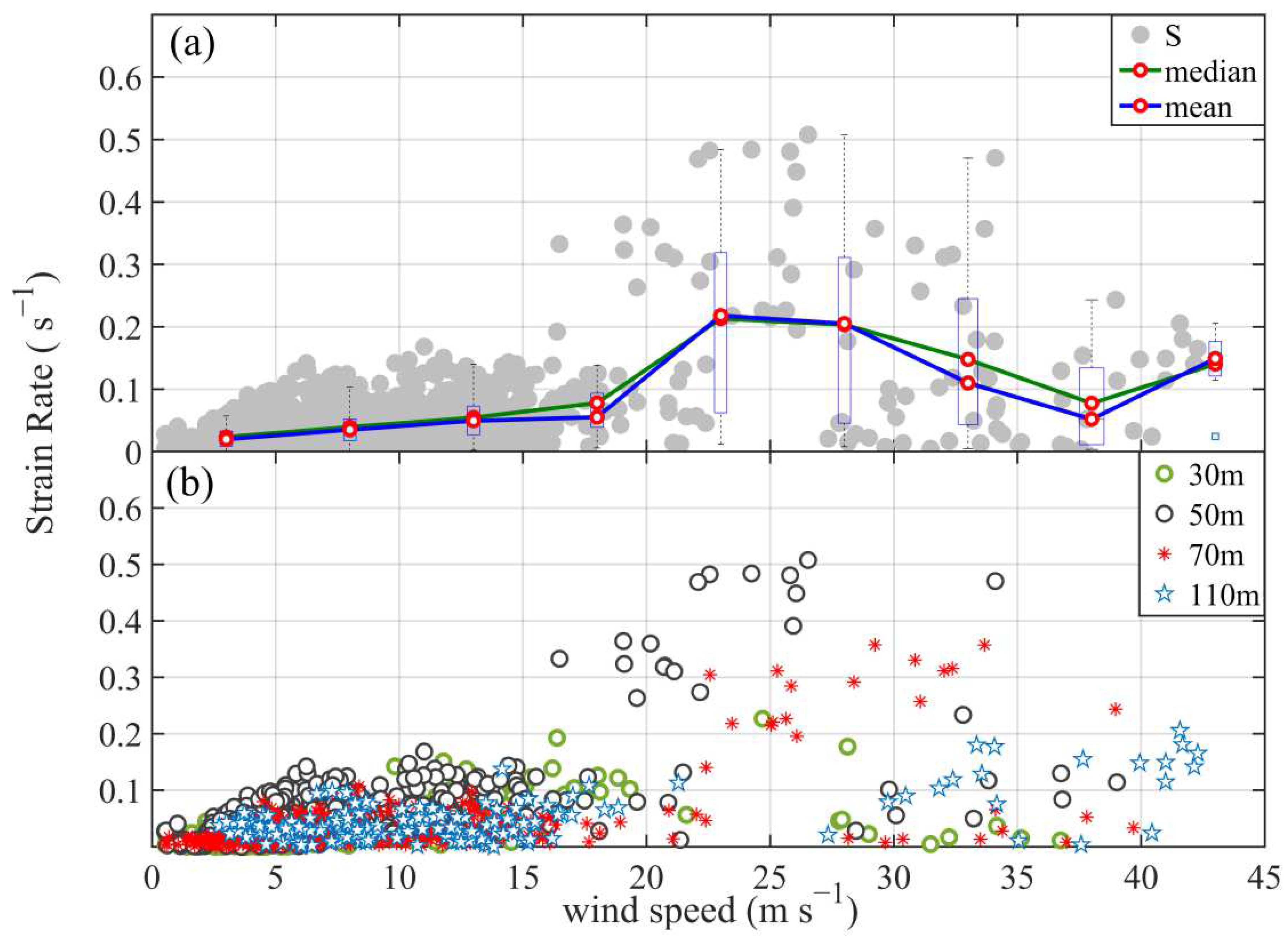
3.7. Variations in the Strain Ratio
The strain ratio (S) as a function of un with the bin averaged mean and median lines of S are shown in Figure 14a. Meanwhile, the S at different layer with un is shown in Figure 14b. Overall, it is evident from Figure 14a that S exhibited a parabolic trend with increasing wind speed from 30 m 70 m heights, while S always increased with increasing un at 110 m height, especially when wind speed exceeded 30 m s−1. The present study was similar to the previous study from Tang et al. [24] when wind speed below 30 m s−1 under 100 m height. The present study also presented the trend under higher wind up to 110 m height.
Furthermore, when increasing the height from 30 m to 110 m, S peaked at 0.22, 0.51, 0.38, and 0.21 s−1 with the corresponding wind speeds being 24.8, 27.0, 22.3, 33.2, and 41.3 m s−1, respectively. This indicates that the maximum of S increased with increasing altitude below a height of 50 m, and then decreased at heights above 50 m. The bin-averaged values of S was 0.035, 0.066, 0.036, and 0.091 s−1 from 30 m to 110 m, respectively. However, as Zhao et al. [25] found S decreased with height up to about 100 m using 356 m tower using landfall, it calls for more observation to be carried out to validate the S trend with altitude.
4. Conclusions and Discussion
Previous studies have focused mainly on TCs over open ocean areas, and few studies have investigated turbulent mixing processes in the high un over the land. In this study, high-frequency wind data were examined using eddy–covariance and flux–gradient methods, which were observed at multiple heights (10–110 m) on the two flux towers in a coastal zone. Small-scale turbulence characteristics were analyzed at high wind speeds of up to 42.5 m s−1 in the near-surface layer of Super Typhoon Maria. The focus was on investigating the characteristics of the turbulent vertical transport and key parameters (|τ|, TKE, VED, Lm, and S) under high wind speeds (>30 m s−1) at five heights. The main conclusions are as follows:
|τ|, TKE, Km, and S increased with increasing un under low and moderate wind conditions, and these decreased with increasing un at high wind speeds (>30 m s−1). The saturated wind speed threshold for the change of |τ|, TKE, and S were about 23 m s−1 when regressed from the medium numbers. Furthermore, our results also imply that the saturated wind speed for the change of τ, TKE, and Km increased with height. The maximum of Km and S increased from the surface to a maximum value at a height of 50 m, and then decreased with greater heights. Additionally, at any given un, |τ|, TKE, and Km were larger than over oceanic areas, and Km was about one to two orders of magnitude bigger than Kt, which may be attributable to differences in surface roughness.
Furthermore, the variations of turbulent parameters with radius in landfalling TC were also analyzed. The |τ|, TKE, and Km values increased with increasing un outside 3 RMW from the TC center but decreased slowly with increasing un located near 1–3 RMW from the TC center. High |τ|, TKE, and Km were basically constant with height at high un of 20.0–42.5 m s−1 within 2–3 RMW from the TC center before typhoon landfall, which indicated turbulent mixing fully suggesting nearly constant flux layers. As compared with Km, Kt with about one to two orders of magnitude smaller than Km showed a clear decrease with increasing wind speed at 1–3 RMW, but little dependence on wind speed outside 3 RMW from the TC center.
The spatial variations in Lm values with un were different outside 3 RMW and within 1–3 RMW from the TC center. In the region of 1–3 RMW before typhoon landfall, Lm increased with un and then began to decrease when un exceeded 38 m s−1. With increasing height from 30 m to 130 m, S peaked at 0.22, 0.51, 0.38, and 0.21 with the corresponding wind speeds being 24.8, 27.0, 22.3, 33.2, and 41.3 m s−1, respectively. The relationships between |τ|, TKE, Km, Lm, and un changed with height and radii from the TC center should be accounted for in sub-grid scale physical processes of momentum fluxes in numerical TC models. It will provide guidance for advance the PBL schemes in improving hurricane intensity forecasts on landfalling and their evolution, especially over land.
In our observation, the analyses showed that the magnitudes of the eddy diffusivity for sensible heat flux was much smaller than those for momentum, the shapes of the vertical distributions of the eddy diffusivities were increasing from the surface to a maximum value, then decreasing with height in the surface layer. The results were consistent with those of Zhang et al. [13] above 500 m height by the CBLAST results, however, it was different from that in earlier theoretical and numerical models. It is typically assumed that the value of Kt is equal to that of Km, or it is calculated using Prandtl and Schmidt numbers (Pr) [42]. In future research, in addition to the momentum flux, more observational data of the heat and moisture fluxes in high winds need to be analyzed, to evaluate the characteristic of Pr to advance our understanding of the air–sea momentum and latent heat exchange under extreme wind conditions [43,44,45,46,47,48].
Although the EC technique is still the most reliable direct method, clearly, turbulence observations are still too limited in the high-wind boundary layer at this point. The vertical variation in Km with un was also consistent with those of Tang et al. [24] using eddy-covariance methods and Zhao et al. [22] using air-craft observation. However, the magnitude was much smaller than that reported by using sodium radar measurements [49]. The TKE was almost constant at a distance of 2–3 times the RMW before landfall, while the TKE increased with decreasing distance to the typhoon center found in the meteorology radar from Shi et al. [50] before Typhoon Maria’s landfall. There still needs to be more turbulence observations and to couple the remotely sensed results to verify the process under extreme wind conditions.
Funding
This research was funded by the Shanghai Municipal Natural Science Foundation with grant number 22ZR1476400, the Key Program for International Science and Technology Cooperation Projects of China with grant number 2017YFE0107700, the National Key Research and Development Program of China with grant number 2020YFE0201900, and the Research Program from the Science Foundation of China with grant numbers 41475060 and 41775065. This research was also supported by the ESCAP/WMO Project (EXOTICCA), the National Natural Science Foundation of China with grant number 42075056, and the Shanghai Science and Technology Research Program with grant number 19dz1200101.
Institutional Review Board Statement
Not applicable.
Informed Consent Statement
Not applicable.
Data Availability Statement
Not applicable.
Acknowledgments
The observational data in this study were from a typhoon experiment observed by Jie Tang, Bingke Zhao, Shuai Zhang and Limin Lin in the Shanghai Typhoon Institute, and we thank the editors and anonymous reviewers for their helpful comments that greatly improved the manuscript.
Conflicts of Interest
The authors declare no conflict of interest.
References
- Emanuel, K.A. An air–sea interaction theory for tropical cyclones. Part I: Steady-state maintenance. J. Atmos. Sci. 1986, 43, 585–604. [Google Scholar] [CrossRef]
- Smith, R.K.; Montgomery, M.T.; Sang, N.V. Tropical cyclone spin-up revisited. Q. J. R. Meteorol. Soc. 2009, 135, 1321–1335. [Google Scholar] [CrossRef] [Green Version]
- Gopalakrishnan, S.G.; Marks, F.; Zhang, J.A.; Zhang, X.; Bao, J.-W.; Tallapragada, V. A study of the impacts of vertical diffusion on the structure and intensity of tropical cyclones using the high resolution HWRF system. J. Atmos. Sci. 2013, 70, 524–541. [Google Scholar] [CrossRef]
- Gopalakrishnan, S.G.; Koch, D.; Upadhayay, S.; DeMaria, M.; Marks, F.; Rappaport, E.N.; Mehra, A.; Tallapragada, V.; Jung, Y.; Alaka, Jr.; et al. 2019 HFIP R&D Activities Summary: Recent Results and Operational Implementation; HFIP Technical Report: HFIP 2018–1.2020; National Oceanic and Atmospheric Administration United States Department of Commerce: Washington, DC, USA, 2019. Available online: http://www.hfip.org/documents/HFIP_AnnualReport_FY2019.pdf (accessed on 13 May 2022).
- Zhang, J.A.; Drennan, W.M. An observational study of vertical eddy diffusivity in the hurricane boundary layer. J. Atmos. Sci. 2012, 69, 3223–3236. [Google Scholar] [CrossRef]
- Zhu, P. Simulation and parameterization of the turbulent transport in the hurricane boundary layer by large eddies. J. Geophys. Res. 2008, 113, D17104. [Google Scholar] [CrossRef]
- Bao, J.-W.; Gopalakrishnan, S.G.; Michelson, S.A.; Marks, F.D.; Montgomery, M.T., Jr. Impact of physics representations in the HWRFX on simulated hurricane structure and pressure–wind relationships. Mon. Wea. Rev. 2012, 140, 3278–3299. [Google Scholar] [CrossRef] [Green Version]
- Kepert, J.D. Choosing a boundary layer parameterization for tropical cyclone modeling. Mon. Wea. Rev. 2012, 140, 1427–1445. [Google Scholar] [CrossRef] [Green Version]
- Zhu, P.; Menelaou, K.; Zhu, Z. Impact of sub-grid scale vertical turbulent mixing on eyewall asymmetric structures and mesovortices of hurricanes. Q. J. R. Meteorol. Soc. 2013, 140, 416–438. [Google Scholar] [CrossRef]
- Zhang, J.A.; Nolan, D.S.; Rogers, R.F.; Tallapragada, V. Evaluating the impact of improvements in the boundary layer parameterizations on hurricane intensity and structure forecasts in HWRF. Mon. Wea. Rev. 2015, 143, 3136–3155. [Google Scholar] [CrossRef]
- Zhang, J.A.; Zhu, P. Effects of vertical eddy diffusivity parameterization on the evolution of landfalling hurricanes. J. Atmos. Sci. 2017, 74, 1879–1905. [Google Scholar] [CrossRef]
- Ming, J.; Zhang, J.A.; Rogers, R.F. Typhoon kinematic and thermodynamic boundary layer structure from dropsonde composites. J. Geophys. Res. Atmos. 2015, 120, 3158–3172. [Google Scholar] [CrossRef]
- Zhang, J.A.; Rogers, R.F.; Tallapragada, V. Impact of parameterized boundary layer structure on tropical cyclone rapid intensification forecasts in HWRF. Mon. Wea. Rev. 2017, 145, 1413–1426. [Google Scholar] [CrossRef]
- Li, X.; Pu, Z. Vertical eddy diffusivity parameterization based on a large-eddy simulation and its impact on prediction of hurricane landfall. Geophys. Res. Lett. 2020, 48, e2020GL090703. [Google Scholar] [CrossRef]
- Zhu, P.; Hazelton, A.; Zhang, Z.; Marks, F.D.; Tallapragada, V. The role of eyewall turbulent transport in the pathway to intensification of tropical cyclones. J. Geophys. Res. Atmos. 2021, 126, e2021JD034983. [Google Scholar] [CrossRef]
- Li, Y.; Zhu, P.; Gao, Z.; Cheung, K.K. Sensitivity of large eddy simulations of tropical cyclone to sub-grid scale mixing parameterization. Atoms. Res. 2022, 265, 105922. [Google Scholar] [CrossRef]
- Nolan, D.S.; Zhang, J.A.; Stern, D.P. Evaluation of planetary boundary layer parameterizations in tropical cyclones by comparison of in-situ data and high resolution simulations of Hurricane Isabel (2003). Part I: Initialization, maximum winds, and outer core boundary layer structure. Mon. Wea. Rev. 2009, 137, 3651–3674. [Google Scholar] [CrossRef]
- Kepert, J.D. The dynamics of boundary layer jets within the tropical cyclone core. Part I: Linear theory. J. Atmos. Sci. 2001, 58, 2469–2484. [Google Scholar] [CrossRef] [Green Version]
- Zhang, J.A.; Marks, F.D.; Montgomery, M.T.; Lorsolo, S. An estimation of turbulent characteristics in the low-level region of intense Hurricanes Allen (1980) and Hugo (1989). Mon. Wea. Rev. 2011, 139, 1447–1462. [Google Scholar] [CrossRef] [Green Version]
- Gopalakrishnan, S.; Hazelton, A.; Zhang, J.A. Improving hurricane boundary layer parameterization scheme based on observations. Earth Space Sci. 2021, 8, e2020EA001422. [Google Scholar] [CrossRef]
- Black, P.G.; Asaro, E.A.D.; Sanford, T.B.; Drennan, W.M.; Zhang, J.A.; French, J.R.; Nüler, P.P.; Terrill, E.J.; Walsh, E.J. Air–sea exchange in hurricanes: Synthesis of observations from the Coupled Boundary Layer Air–Sea Transfer experiment. B. Meteorol. Soc. 2007, 88, 357–374. [Google Scholar] [CrossRef] [Green Version]
- Zhao, Z.K.; Chan, P.W.; Wu, N.; Zhang, J.A.; Hon, K.K. Aircraft observations of turbulence characteristics in the tropical cyclone boundary layer. Bound. Layer Meteorol. 2020, 174, 493–511. [Google Scholar] [CrossRef]
- Katz, J.; Zhu, P. Evaluation of surface layer flux parameterizations using in-situ observations. Atmos. Res. 2017, 194, 150–163. [Google Scholar] [CrossRef]
- Tang, J.; Zhang, J.A.; Aberson, S.D.; Marks, F.D.; Lei, X. Multilevel tower observations of vertical eddy diffusivity and mixing length in the tropical cyclone boundary layer during landfalls. J. Atmos. Sci. 2018, 75, 3159–3168. [Google Scholar] [CrossRef]
- Zhao, Z.; Gao, R.; Zhang, J.A.; Zhu, Y.; Liu, C.; Chan, P.W.; Wan, Q. Observations of Boundary Layer Wind and Turbulence of a Landfalling Tropical Cyclone. 20 August 2021, PREPRINT (Version 1) available at Research Square. Available online: https://www.researchgate.net/publication/354043506_Observations_of_Boundary_Layer_Wind_and_Turbulence_of_a_Landfalling_Tropical_Cyclone (accessed on 28 May 2022).
- Li, L.; Xiao, Y.; Zhou, H.; Xing, F.; Song, L. Turbulent wind characteristics in typhoon Hagupit based on field measurements. Int. J. Distrib. Sens. Netw. 2018, 14. [Google Scholar] [CrossRef]
- Xia, D.; Dai, L.; Lin, L.; Wang, H.; Hu, H. A Field Measurement based Wind Characteristics Analysis of a Typhoon in Near-ground Boundary Layer. Atmosphere 2021, 12, 873. [Google Scholar] [CrossRef]
- Lee, X.; Massman, W.; Law, B. Handbook of Micrometeorology: A Guide for Surface Flux Measurement and Analysis; Kluwer Academic Publishers: New York, NY, USA, 2004; pp. 33–66. [Google Scholar]
- Qin, Z.; Xia, D.; Dai, L.; Zheng, Q.; Lin, L. Investigations on wind characteristics for typhoon and monsoon wind speeds based on both stationary and non-stationary models. Atmosphere 2022, 13, 178. [Google Scholar] [CrossRef]
- Ying, M.; Zhang, W.; Yu, H.; Lu, X.; Feng, J.; Fan, Y.; Zhu, Y.; Chen, D. An overview of the China Meteorological Administration tropical cyclone database. J. Atmos. Ocean Tech. 2014, 31, 287–301. [Google Scholar] [CrossRef] [Green Version]
- Bao, X.; Wu, L.; Zhang, S.; Li, Q.; Lin, L.; Zhao, B.; Wu, D.; Xia, W.; Xu, B. Distinct raindrop size distributions of convective inner- and outer-rainband rain in Typhoon Maria (2018). J. Geophys. Res. Atmos. 2020, 125, e2020JD032482. [Google Scholar] [CrossRef]
- Stull, R.B. An Introduction to Boundary Layer Meteorology; Kluwer Academic Publishers: Dordrecht, The Netherlands, 1988; p. 670. [Google Scholar]
- Schmid, H.P.; Grimmond, C.S.B.; Cropley, F.; Offerle, B.; Su, H.B. Measurements of CO2 and energy fluxes over a mixed hardwood forest in the mid-western United States. Agric. Forest Meteorol. 2000, 103, 357–374. [Google Scholar] [CrossRef]
- Foken, T.; Göockede; Mauder, M.; Mahrt, L.; Amiro, B.; Munger, W. Handbook of Micrometeorology: Post-Field Data Quality Control; Lee, X., Massman, W., Law, B., Eds.; Springer: Dordrecht, The Netherlands, 2005; pp. 181–208. [Google Scholar]
- Monin, A.S.; Obukhov, A.M. Basic laws of turbulent mixing in the surface layer of the atmosphere. Akad. Nauk. SSSR. Geofiz. Inst. Trudy 1954, 151, 163–187. [Google Scholar]
- Fortuniak, K.; Pawlak, W. Selected Spectral Characteristics of Turbulence over an Urbanized Area in the Centre of Łód’z, Poland. Bound. Layer Meteorol. 2015, 154, 137–156. [Google Scholar] [CrossRef] [Green Version]
- Kaimal, J.C.; Wyngaard, J.C.; Coté, O.R. Spectral characteristics of surface-layer turbulence. Q.J.R. Meteorol. Soc. 1972, 98, 563–589. [Google Scholar] [CrossRef]
- Ortiz-Suslow, D.G.; Kalogiros, J.; Yamaguchi, R.; Wang, Q. An evaluation of the constant flux layer in the atmospheric flow above the wavy air-sea interface. J. Geophys. Res. Atmos. 2021, 126, e2020JD032834. [Google Scholar] [CrossRef]
- Kaimal, J.C.; Finnigan, J.J. Atmospheric Boundary Layer Flows: Their Structures and Measurements; Oxford University Press: Oxford, UK, 1994. [Google Scholar]
- Grachev, A.A.; Leo, L.S.; Fernando, H.J.S.; Fairall, C.W.; Creegan, E.; Blomquist, B.W.; Christman, A.J.; Hocut, C.M. Air-sea/land interaction in the coast. Bound. Layer Meteorol. 2018, 167, 181–210. [Google Scholar] [CrossRef]
- Grachev, A.A.; Krishnamurthy, R.; Fernando, H.J.S.; Fairall, C.W.; Bardoel, S.L.; Wang, S. Atmospheric turbulence measurements at a coastal zone with and without Fog. Bound. Layer Meteorol. 2021, 181, 395–422. [Google Scholar] [CrossRef]
- Zhang, J.A.; Rogers, R.F. Effects of parameterized boundary layer structure on hurricane rapid intensification in shear. Mon. Wea. Rev. 2019, 147, 853–871. [Google Scholar] [CrossRef]
- Lükö, G.; Torma, P.; Weidinger, T. Intra-Seasonal and Intra-Annual Variation of the Latent Heat Flux Transfer Coefficient for a Freshwater Lake. Atmosphere 2022, 13, 352. [Google Scholar] [CrossRef]
- Dudorova, N.V.; Belan, B.D. The Energy Model of Urban Heat Island. Atmosphere 2022, 13, 457. [Google Scholar] [CrossRef]
- Yang, L.; Qian, F.; Song, D.-X.; Zheng, K.-J. Research on Urban Heat-Island Effect. Procedia Eng. 2016, 169, 11–18. [Google Scholar] [CrossRef]
- Kalina, E.A.; Biswas, M.K.; Zhang, J.A.; Newman, K.M. Sensitivity of an Idealized Tropical Cyclone to the Configuration of the Global Forecast System–Eddy Diffusivity Mass Flux Planetary Boundary Layer Scheme. Atmosphere 2021, 12, 284. [Google Scholar] [CrossRef]
- Do Nascimento, A.C.L.; Galvani, E.; Gobo, J.P.A.; Wollmann, C.A. Comparison between Air Temperature and Land Surface Temperature for the City of São Paulo, Brazil. Atmosphere 2022, 13, 491. [Google Scholar] [CrossRef]
- Elmarakby, E.; Khalifa, M.; Elshater, A.; Afifi, S. Tailored methods for mapping urban heat islands in Greater Cairo Region. Ain Shams Eng. J. 2021. [Google Scholar] [CrossRef]
- Li, J.; Collins, R.; Lu, X.; Williams, B. Lidar observations of instability and estimates of vertical eddy diffusivity induced by gravity wave breaking in the Arctic mesosphere. J. Geophys. Res. Atmos. 2021, 126, e2020JD033450. [Google Scholar] [CrossRef]
- Shi, W.; Tang, J.; Chen, Y.; Chen, N.; Liu, Q.; Liu, T. Study of the Boundary Layer Structure of a Landfalling Typhoon Based on the Observation from Multiple Ground-Based Doppler Wind Lidars. Remote Sens. 2021, 13, 4810. [Google Scholar] [CrossRef]
Figure 1.
Track of Typhoon Maria and the location, exposure, and instruments on the two eddy covariance flux towers. The coastal observation towers are marked by the yellow arrow. (a) Photograph of the coastal observation tower approximately 10 m from the coastline (Figure 1a), which is referred to as the lower tower in this study. The CAST anemometers on the lower tower are 10, 30, 50, and 70 m above the ground (60, 80, 100, and 120 m above sea level). (b) Photograph of the coastal observation tower at the top of the hill, which is referred to as the higher tower in this study. The CAST anemometers on the higher tower are 50 m above the ground (170 m above sea level).

Figure 2.
(a) Cumulative frequency curves (ogive) of the vertical velocity w with the along−wind u and cross−wind v components. The cospectra densities of the vertical velocity (w) with the along-wind (u) and cross-wind (v) components and ultrasonic virtual temperature (T) at (b) 10 m, (c) 30 m, (d) 50 m, (e) 70 m, and (f) 110 m. Ten-minute averaged data are for Typhoon Maria (2018) from 0000 local standard time (LST) 10 July to 0000 LST 12 July 2018.

Figure 3.
Normalized logarithmic along-wind spectrum plotted against the non-dimensional frequency, f = n(z)/u at (a) 10 m, (b) 30 m, (c) 50 m, (d) 70 m, and (e) 110 m. Short red solid lines indicate the along-wind spectrum of slopes for the inertial subrange. Twenty hertz raw data were for Typhoon Maria (2018) from 0000 local standard time (LST) 10 July to 0000 LST 12 July 2018.

Figure 4.
Plots of the normalized standard deviations of the longitudinal wind velocity components (/) in log-log scales versus the stability parameter (z/L) under unstable (or CBL, <0,) and stable (or UBL, 𝜁 > 0) stratification conditions for the 10-min-averaged onshore data collected during Typhoon Maria’s landfall (10–12 July 2018). The black dashed lines correspond to for 𝜁 < 0 and for 𝜁 > 0 (Kaimal and Finnigan [39]).

Figure 5.
Plots of the normalized standard deviations of the lateral wind velocity components (/) in log−log scales versus the stability parameter (z/L) under unstable (or CBL, <0,) and stable (or UBL, 𝜁 > 0) stratification conditions for the 10-min-averaged onshore data collected during Typhoon Maria’s landfall (10–12 July 2018). The black dashed lines correspond to for 𝜁 < 0 and for 𝜁 > 0 (Kaimal and Finnigan [39]).

Figure 6.
Plots of the normalized standard deviations of the longitudinal wind velocity components (/) in log–log scales versus the stability parameter (z/L) under unstable (or CBL, <0,) and stable (or UBL, 𝜁 > 0) stratification conditions for the 10-min averaged onshore data collected during Typhoon Maria’s landfall (10–12 July 2018). The black dashed lines correspond to for 𝜁 < 0 and for 𝜁 > 0 (Kaimal and Finnigan [39]).

Figure 7.
Temporal changes in the 10-min averaged wind speed (un) and wind direction (WD) obtained from the sonic anemometers on the five heights [(a) 110 m, (b) 70 m, (c) 50 m, (d) 30 m, and (e) 10 m of the two towers during Typhoon Maria (2018). Section A is the time period before typhoon landfall on 11 July and Section B is the time period after typhoon landfall.

Figure 8.
(a) Time-series of the 10-min averaged wind speed and (b) turbulent kinetic energy (TKE), (c) air pressure of the typhoon center and precipitation during landfall, and (d) distance of the typhoon center to the tower and radar reflectivities (dBz) observed nearby flux towers from 10 to 12 July (distance data are from http://www.typhoon.gov.cn/, accessed on 1 January 2020).

Figure 9.
Plots of the (a) momentum flux and (b) turbulent kinetic energy at the five height levels during Typhoon Maria. Plots of the (c) momentum fluxes and (d) turbulent kinetic energy as a function of wind speeds at the five heights during landfall of Typhoon Maria. The blue line with the red circles is the bin median average at 5 m s−1 intervals of un from the observations. The yellow line with red circle is the bin mean average at 5 m s−1 intervals of un from the observations.

Figure 10.
Plots of the (a) momentum fluxes and (b) turbulent kinetic energy versus wind speed as a function of the TC radius normalized by the maximum wind speed radius (RMW). The data were classified into seven categories according to the TC radius normalized by RMW. Histograms of the (c) turbulent kinetic energy and (d) momentum fluxes. Each color represents the seven categories defined by the TC radius normalized to RMW.

Figure 11.
Vertical eddy diffusivity of momentum (Km) as a function of wind speed (un). The blue line with the red circles is the bin median averaged Km at 5 m s−1 intervals of un from the observations. The yellow line with the red circles is the bin mean averaged Km at 5 m s−1 intervals of un from the observations (a). The data were classified into seven categories according to their distance from the typhoon center (b).

Figure 12.
Vertical eddy diffusivity of heat (Kt) as a function of wind speed (un). The blue line with red circles is the bin median average Kt at 5 m s−1 intervals of un from the observations. The yellow line with the red circle represents the bin mean averaged Kt with 5 m s−1 interval of un from the observations (a). The data were classified into seven categories according to their distance from the typhoon center (b).

Figure 13.
(a) Vertical mixing length (Lm) as a function of wind speed (un). The data were classified into seven categories according to their distance from the typhoon center. (b) The blue line with the red circles is the bin median average Kt at 5 m s−1 intervals of un from the observations. The green line with red circles is the bin mean average Kt at 5 m s−1 intervals of un from the observations.

Figure 14.
(a) S as a function of un during landfall of Typhoon Maria. The blue line with the red circles is the bin median average S at 5 m s−1 intervals of un from the observations. The yellow line with red circles is the bin mean average S at 5 m s−1 intervals of un from the observations. (b) Strain rate (S) at four heights plotted versus wind speed (un) during landfall of Typhoon Maria. The strain rate was calculated using Equation (7).


Table 1.
Maximum 10-min mean wind speed and directions during Typhoon Maria in 2018.
| First Peak | Second Peak | |||
|---|---|---|---|---|
| Onshore (52.5–227.5°) | Offshore (272–5°) | |||
| Instrument Height (m) | Wind Speed (m s−1) | Wind Direction (°) | Wind Speed (m s−1) | Wind Direction (°) |
| 10 | 16.57 | 300.22 | 36.51 | 48.28 |
| 30 | 19.05 | 316.41 | 36.79 | 51.17 |
| 50 | 22.26 | 234.08 | 39.06 | 47.72 |
| 70 | 29.61 | 243.53 | 39.67 | 42.17 |
| 110 | 21.28 | 329.92 | 42.27 | 54.50 |
Publisher’s Note: MDPI stays neutral with regard to jurisdictional claims in published maps and institutional affiliations. |
© 2022 by the author. Licensee MDPI, Basel, Switzerland. This article is an open access article distributed under the terms and conditions of the Creative Commons Attribution (CC BY) license (https://creativecommons.org/licenses/by/4.0/).
Share and Cite
MDPI and ACS Style
Chen, C. Vertical Eddy Diffusivity in the Tropical Cyclone Boundary Layer during Landfall. Atmosphere 2022, 13, 982. https://doi.org/10.3390/atmos13060982
AMA Style
Chen C. Vertical Eddy Diffusivity in the Tropical Cyclone Boundary Layer during Landfall. Atmosphere. 2022; 13(6):982. https://doi.org/10.3390/atmos13060982
Chicago/Turabian StyleChen, Chen. 2022. "Vertical Eddy Diffusivity in the Tropical Cyclone Boundary Layer during Landfall" Atmosphere 13, no. 6: 982. https://doi.org/10.3390/atmos13060982
Note that from the first issue of 2016, this journal uses article numbers instead of page numbers. See further details here.