Article

Genetic Algorithm-Optimized Extreme Learning Machine Model for Estimating Daily Reference Evapotranspiration in Southwest China

1
State Key Laboratory of Hydraulics and Mountain River Engineering, College of Water Resource and Hydropower, Sichuan University, Chengdu 610065, China
2
Institute of Environment and Sustainable Development in Agriculture, Chinese Academy of Agricultural Sciences, Beijing 100081, China
3
Key Laboratory of Agricultural Soil and Water Engineering in Arid and Semiarid Areas, Ministry of Education, Northwest A & F University, Yangling, Xianyang 712100, China
*
Author to whom correspondence should be addressed.
Atmosphere 2022, 13(6), 971; https://doi.org/10.3390/atmos13060971
Submission received: 28 April 2022 / Revised: 7 June 2022 / Accepted: 10 June 2022 / Published: 15 June 2022
(This article belongs to the Section Biosphere/Hydrosphere/Land–Atmosphere Interactions)

Abstract

:
Reference evapotranspiration (ET0) is an essential component in hydrological and ecological processes. The Penman–Monteith (PM) model of Food and Agriculture Organization of the United Nations (FAO) model requires a number of meteorological parameters; it is urgent to develop high-precision and computationally efficient ET0 models with fewer parameter inputs. This study proposed the genetic algorithm (GA) to optimize extreme learning machine (ELM), and evaluated the performances of ELM, GA-ELM, and empirical models for estimating daily ET0 in Southwest China. Daily meteorological data including maximum temperature (Tmax), minimum temperature (Tmin), wind speed (u2), relative humidity (RH), net radiation (Rn), and global solar radiation (Rs) during 1992–2016 from meteorological stations were used for model training and testing. The results from the FAO-56 Penman–Monteith formula were used as a control group. The results showed that GA-ELM models (with R2 ranging 0.71–0.99, RMSE ranging 0.036–0.77 mm·d−1) outperformed the standalone ELM models (with R2 ranging 0.716–0.99, RMSE ranging 0.08–0.77 mm·d−1) during training and testing, both of which were superior to empirical models (with R2 ranging 0.36–0.91, RMSE ranging 0.69–2.64 mm·d−1). ET0 prediction accuracy varies with different input combination models. The machine learning models using Tmax, Tmin, u2, RH, and Rn/Rs (GA-ELM5/GA-ELM4 and ELM5/ELM4) obtained the best ET0 estimates, with R2 ranging 0.98–0.99, RMSE ranging 0.03–0.21 mm·d−1, followed by models with Tmax, Tmin, and Rn/Rs (GA-ELM3/GA-ELM2 and ELM3/ELM2) as inputs. The machine learning models involved with Rn outperformed those with Rs when the quantity of input parameters was the same. Overall, GA-ELM5 (Tmax, Tmin, u2, RH and Rn as inputs) outperformed the other models during training and testing, and was thus recommended for daily ET0 estimation. With the estimation accuracy, computational costs, and availability of input parameters accounted, GA-ELM2 (Tmax, Tmin, and Rs as inputs) was determined to be the most effective model for estimating daily ET0 with limited meteorological data in Southwest China.

1. Introduction

Reference evapotranspiration (ET0) is an important component in hydrological and ecological processes and a key parameter in determining crop water requirements for agricultural water management [1,2]. The Penman–Monteith (PM) model, based on both thermodynamics and dynamics, is of great rigorous theory and accurate estimation. Therefore, PM model has been recommended by the Food and Agriculture Organization of the United Nations (FAO) as the standard equation for estimating ET0 and is thus widely accepted [3]. However, the FAO-56 PM model requires a number of meteorological parameters for a long period of time as input variables, and its data integrity requirements are extremely high, which limited its development in some areas where complete meteorological data are lacking. Hence, it is urgent to develop high-precision ET0 models with fewer parameter inputs.
Many ET0 empirical models with limited meteorological inputs have been developed, e.g., temperature-based models, radiation-based models, and mass transfer-based models [4]. Hargreaves model [5] is a classic temperature-based model for ET0 estimation in virtue of its popularization and high prediction accuracy with only maximum and minimum temperatures and radiation data introduced. According to Priestley, Taylor, and Samani [6,7], about 80% of ET0 calculations can be explained by air temperature and solar radiation, leading to accurate prediction in ET0 by using radiation-based models. Feng et al. [8] evaluated the computational performance of five ET0 empirical models (Hargreaves model, Modified Hargreaves model, Makkink model, Priestley–Taylor model and Ritchie model) in the humid region of Southwest China, and found that the radiation-based empirical models (Priestley–Taylor and Ritchie model) had higher prediction accuracy. The Romanenko model [9] is the mass transfer-based model that introduced relative humidity (RH) based on temperature parameter. The results of ET0 prediction by using data from 203 weather stations distributed across Brazil showed that the addition of relative humidity as an input for ET0 models yielded a better prediction performance at a low cost. Nonetheless, applying them directly to other regions usually reduces the estimation accuracy of models because the empirical models are susceptible to the climate zone environment and geographic location. Djaman et al. [10] evaluated 16 empirical models for estimating ET0, and found that the empirical models were overestimated or underestimated. Zhang et al. [11] found that the calibrated Makkink model had better performance on ET0 prediction than uncalibrated models.
Artificial intelligence techniques have developed rapidly in recent decades and have been applied in many fields. Due to their excellent performance in tackling nonlinear regression problems, machine learning models have been widely used to reveal the complex hydrological phenomena and estimate ET0 [12,13,14]. Tabari et al. [15] evaluated the performances of support vector machine (SVM), adaptive neuro-fuzzy inference system (ANFIS), multiple linear regression (MLR), multiple non-linear regression (MNLR), four temperature-based models, and eight radiation-based empirical models for ET0 estimation in the semi-arid climate of Iran. It was found that the SVM and ANFIS models performed best. Chen et al. [16] used three deep learning methods, namely deep neural network (DNN), temporal convolution neural network (TCN), long short-term memory neural network (LSTM), and two machine learning models, namely SVM and random forest (RF), to predict daily ET0 under limited meteorological data conditions in the Northeast Plain of China. The results showed that the prediction accuracy of deep learning and machine learning models was higher than that of empirical models based on radiation and humidity data. The extreme learning machine (ELM) model, proposed by Huang et al. [17], consists of three layers: an input layer, a hidden layer (neurons), and an output layer, and can minimize the computational costs. Abdullah et al. [18] analyzed the performance of ELM and back propagation neural network (BPNN) models in estimating ET0 in Iraq. They found that the two models had similar accuracy, but ELM showed better computational efficiency. Chia et al. [19] hybridized the ELM with three swarm-based optimization algorithms, namely the particle swarm optimization (PSO), the moth-flame optimization (MFO), and the whale optimization algorithm (WOA), to predict ET0 in East Malaysia. It was concluded that WOA-ELM outperformed PSO-ELM and MFO-ELM. Wu et al. [20] evaluated the performances of four bio-inspired algorithms (i.e., genetic algorithm (GA), ant colony optimization (ACO), cuckoo search algorithm (CSA), and flower pollination algorithm (FPA)), and optimized extreme learning machine (ELM) models for estimating daily ET0. The results advocated the capability of bio-inspired optimization algorithms, especially the FPA and CSA algorithms, for improving the performance of the conventional ELM model in daily ET0 prediction in contrasting climates of China.
Southwest China is not only an important grain production base, but also an ecological defense in China. In recent years, the frequency and intensity of seasonal droughts have been increasing in Southwest China due to global warming. In the future, water resources in Southwest China will become more fragile under the impacts of climate change and human activities, resulting in decreased precipitation and intensified dry-hot weather [21,22]. It is apparent from the related reviews that the ELM model has a good applicability for ET0 estimations. Although the high prediction accuracy plays a very important role when employing the ELM model, the less computational effort is also essential to consider [23]. Therefore, applying optimization algorithms for ELM model parameters tuning provides more reliable ET0 estimations, which is of great significance to achieve precise irrigation, optimize water resources management, and maintain ecological security in Southwest China. This study employed GA to optimize the ELM model to improve the accuracy for estimating daily ET0, and reduce the calculation cost of ELM model under different input combinations. Therefore, the study aims were to: (1) build GA-ELM and ELM models for modeling ET0 in Southwest China based on daily meteorological data during 1992–2016; (2) optimize weights and thresholds of GA-ELM model with five input combinations; (3) explore the optimal daily ET0 forecasting model of ELM, GA-ELM, and empirical models in Southwest China to provide a scientific basis for agricultural water management.

2. Materials and Methods

2.1. Study Area and Data Sets

Southwest China (20°54′–36°53′ N, 78°28′–112°04′ E) covers 2.6 million km2, accounting for 27% of China’s territorial area. The climate in the Southwest China is dominated by subtropical monsoon and plateau mountain climates. The altitude of the study area varies greatly, and the terrain structure is changeable and complex. There are mainly basins, mountainous, and hilly areas as well as plateau mountain areas. Southwest China is rich in water resources, with an annual precipitation of 800 mm. However, the annual precipitation varies significantly in space, with decreasing tendency from east to west.
Considering the topography, elevation, and landform characteristics, Southwest China is further divided into five sub-zones [24,25], i.e., the Qinghai–Tibet Plateau (QTP), the Northwest Sichuan Plateau (NSP), the Sichuan Basin (SB), the Yunnan–Kweichow plateau (YGP), and the Guangxi Basin (GB) (Figure 1). QTP is an ecological fragile region with an average altitude of 4000 m and sparse vegetation. NSP is one of the five largest pastoral areas in China and the largest animal husbandry base in Sichuan. The SB is one of the main grain-producing areas in China, with dense population and developed agriculture. YGP is one of the four plateaus in China, and there are many types of disastrous weather. The average elevation of the GB is less than 200 m, which is high in the northwest and low in the southeast.
The daily meteorological data of fifteen representative meteorological stations in Southwest China from 1992 to 2016 were selected from the China Meteorological Administration (http://data.cma.cn, accessed on 1 November 2021), including maximum temperature (Tmax), minimum temperature (Tmin), wind speed (u2), relative humidity (RH), net surface radiation (Rn), and global solar radiation (Rs). The annual mean values of meteorological parameters at the studied meteorological stations can be found in Table 1.

2.2. Penman–Monteith Model

The PM model incorporates the aerodynamic effects and principle of water balance, and has been recommended by FAO as the reference model for ET0 calculation because of its rigorous theory and high calculation accuracy. The specific expression [3] of the formula is:
E T 0 = 0.408 ( R n G ) + γ 900 T m e a n + 273 u 2 ( e s e a ) + γ ( 1 + 0.34 u 2 )
where ET0 is reference evapotranspiration (mm·d−1); Rn is the net surface radiation (MJ·m−2·d−1); G is the soil heat flux density (MJ·m−2·d−1); Tmean is the mean daily air temperature (°C); u2 is the wind speed at 2 m height (m·s−1); es is saturation vapor pressure (kPa);  ea is actual vapor pressure (kPa); Δ is the slope of vapor pressure curve; Υ is the psychrometric constant (kPa/°C). The detailed calculation processes can be found in the FAO-56 [3].

2.3. Empirical Models

2.3.1. Romanenko Model

Romanenko [9] is an ET0 prediction model based on temperature and humidity, and the specific expression is as follows:
E T 0 = 0.00006 ( T m e a n + 25 ) 2 ( 100 R H )
where Tmean is the mean daily air temperature (°C); RH is the relative humidity (%).

2.3.2. Makkink Model

Makkink [26] is a radiation-based model for predicting ET0. The specific expression is as follows:
E T 0 = 0.61 ( + γ ) R s λ 0.12
where Δ, γ and Rn were defined in Equation (1). Rs is the global solar radiation (MJ·m−2·d−1); λ is the latent heat of vaporization (MJ/kg).

2.3.3. Tabari Model

Hossein Tabari [27] proposed an ET0 prediction model based on solar radiation under humid conditions:
E T 0 = 0.156 R s 0.0112 T m a x + 0.0733 T m i n 0.478
where Tmax and Tmin are maximum and minimum air temperatures (°C), respectively.

2.3.4. Irmak–Allen Model

Irmak [28] proposed an ET0 prediction model based on net surface radiation in humid climate:
E T 0 = 0.489 + 0.289 R n + 0.023 T m e a n

2.3.5. Priestley–Taylor Model

Priestley and Taylor [6] derived the Priestley–Taylor formula from solar radiation and soil heat flux, and the specific expression is:
E T 0 = 1.26 + γ R n G λ
where Δ, γ, Rn and G were defined in Equation (1).

2.4. Extreme Learning Machine and Optimization Algorithms

2.4.1. Extreme Learning Machine

The ELM model, proposed by Holland [17], is a single-hidden layer feedforward neural network. The principle of ELM is that the weight and threshold are randomly generated, and the number of neurons is set in the hidden layer. Then, the unique and optimal solution can be obtained by simple matrix calculation [8]. ELM model has the advantages of faster learning speed and better generalization performance, which can not only solve the problems of regression and fitting, but also has been widely used in classification, pattern recognition and other fields. As shown in Figure 2, the ELM model consists of three layers: input layer, hidden layer, and output layer. Further details about the ELM model can be found in reference [17].

2.4.2. Extreme Learning Machine Optimized by Genetic Algorithm

Genetic algorithm (GA) was developed by Holland [29] to search the optimal solution by simulating the process of biological evolution, and is usually used to deal with nonlinear optimization problems [30]. The basic logic of GA is Darwin’s evolution theory. GA begins with a population representing a potential solution to an optimization problem, while the population consists of many individuals with genetic codes. The principle of GA is to convert the solution of the problem into chromosomes. According to the principle of survival of the fittest, the information in chromosomes is transformed by selection, crossover, and mutation, and eventually evolves into the target chromosome. In other words, the evolution of generations produces the approximate optimal solution which is close to the objective function.
The internal parameters of the ELM were randomly initialized, leading to poor stability and generalization performance. Estimation of the kernel-based ELM can be improved by fine-tuning the internal parameters. Specifically, GA can be applied to optimize the parameters of the ELM model, thereby improving the performances of the models because it is capable of deducting the optimal solutions and improving the computational speed. In GA-ELM model, the input weights and node thresholds of hidden layer are chromosome vectors of GA. In a word, GA was used to optimize the optimal input weights and thresholds of ELM. The optimization process is presented in Figure 3. For more details on GA-ELM, see reference [29].

2.5. Input Combinations of Meteorological Parameters

In this study, the daily data during 1992–2011 from 15 representative meteorological stations were used to train the ELM and GA-ELM model, and the rest of the data were used for testing. As shown in Figure 4, the correlation between Rn, Rs, and ET0 was highest, followed by that between temperature and ET0. The correlation between u2, RH, and ET0 was lowest, which was consistent with the results of Chia and Sharma [19,31]. Previous studies have showed that global solar radiation and temperature were significant meteorological factors affecting ET0 in Southwest China [8,25,32]. Therefore, the temperature-related and radiation-related factors were selected as the input parameters in this study. The number and combination of input variables will affect the performance of the machine learning model. In the case of limited meteorological parameters, parameters with reliable correlation can effectively improve the accuracy of models for estimating daily ET0 [33]. This study proposed appropriate input combinations based on the correlation between different climate variables and ET0. The input combinations are shown in Table 2.

2.6. Model Evaluation

Five commonly used statistical indicators were used to analyze and compare the accuracy and performance of different models in estimating daily ET0, including coefficient of determination (R2), root mean square error (RMSE), relative root mean square error (RRMSE), mean absolute error (MAE), and global performance indicator (GPI), which were defined in the following equations:
R 2 = [ i = 1 n ( X i x ¯ ) ( Y i Y ¯ ) ] 2 i = 1 n ( X i X ¯ ) 2 i = 1 n ( Y i Y ¯ ) 2
R M S E = 1 n i = 1 n ( Y i X i ) 2
R R M S E = 1 n i = 1 n ( Y i X i ) 2 X i ¯
M A E = 1 n i = 1 n | Y i X i |
G P I i = i = 1 4 α k ( Z i k Z k )
where Xi and Yi are the measured and predicted ET0 values, respectively; X i ¯ and Y i ¯ are the corresponding mean ET0 values; n is the number of data. GPIi is GPI values of the model i; k is the verification factor; Zik is the value of k for model i; Zk is the median of the k. αk equals –1 for k being RMSE, RRMSE and MAE, and equals 1 for k being R2. The higher R2 is close to 1, the better models perform; the closer RMSE, RRMSE, and MAE are to 0, the smaller the models’ simulation error. The best-performing model with the highest GPI was ranked No.1, while the model corresponding to the lowest GPI was ranked No.15.

3. Results

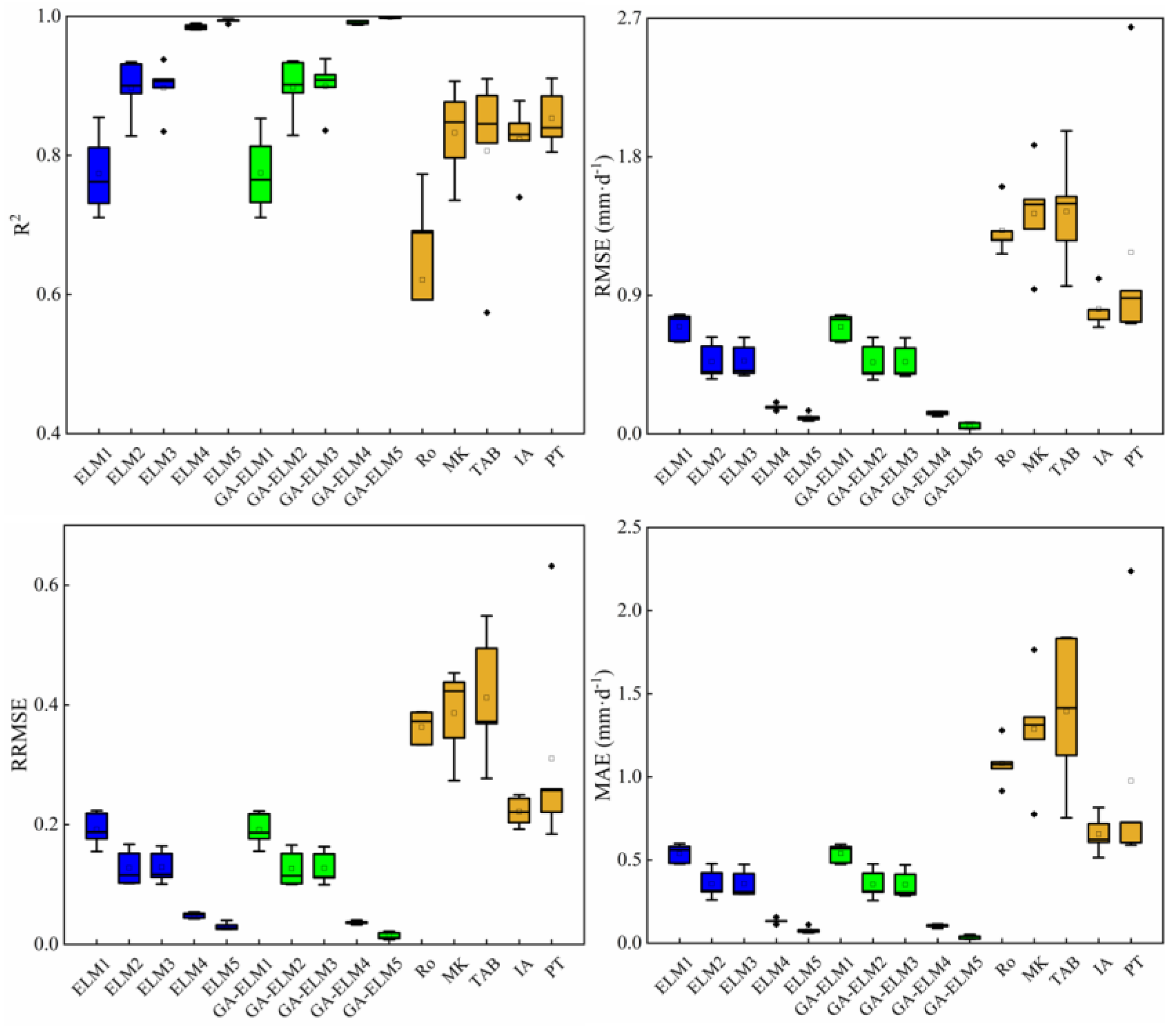
3.1. Performances of Reference Evapotranspiration Models in the Five Zones

The statistical results of ELM, GA-ELM, and empirical models for predicting ET0 in each sub-zone during training and testing are presented in Table 3. It can be observed from Table 3 that R2 and RMSE of ELM models were 0.59–0.99, 0.08–0.77 mm·d−1, respectively; the corresponding values of GA-ELM models were 0.56–0.99, 0.03–0.77 mm·d−1, respectively; the corresponding values of empirical models were 0.36–0.91, 0.69–2.64 mm·d−1, respectively. GA-ELM models showed good prediction accuracy in each sub-zone, with the highest prediction accuracy, followed by the ELM models, while the empirical models had the worst overall accuracy.
As seen from Table 3, GA-ELM and ELM models with complete input showed optimal prediction accuracy in each sub-zone during training and testing. The R2 and RMSE of GA-ELM and ELM models were 0.98–0.99, 0.03–0.21 mm·d−1, respectively; the corresponding values of machine learning models with three parameters inputs were 0.83–0.98, 0.34–0.63 mm·d−1, models with two parameters inputs were 0.56–0.95, 0.60–0.77 mm·d−1, respectively.
The prediction accuracy of two-input models was the worst, and the GPI rank of two-input models in SB and YGP was even lower than that of IA and PT models, respectively. The accuracy of three-input models was significantly improved compared with that of the two-input models, while the accuracy of the complete input models was slightly higher than that of the three-parameter input models, indicating that three-input models can also predict ET0 with acceptable accuracy in areas where meteorological parameters were difficult to obtain completely.
ELM and GA-ELM models involved with Rn always showed more accurate results than those involved with Rs under the same quantity of inputs. With Tmax, Tmin, Rs/Rn, u2, and RH as inputs, the R2 of GA-ELM5 and ELM5 models were above 0.99, and the RMSE of those ranged 0.03–0.07 mm·d−1/0.08–0.15 mm·d−1, respectively; the R2 of GA-ELM4 and ELM4 models were above 0.98, and the RMSE of those ranged 0.110–0.15 mm·d−1/0.14–0.21 mm·d−1, respectively. So, the rank was GA-ELM5> GA-ELM4, ELM5> ELM4. With Tmax, Tmin, Rs/Rn, u2, and RH as inputs, GA-ELM3 involved with Rn exhibited the best prediction accuracy in QTP, NSP, SB and GB; GA-ELM2 involved with Rs outperformed the other models in YGP. Similar results were shown in empirical models. The accuracy of the IA and PT model were better than that of other empirical models. IA model was the optimal empirical model in NSP, SB, and GB. The PT model outperformed the other empirical models in QTP and YGP.
It can be observed from Table 3 that the studied models in terms of prediction accuracy during training and testing were ranked in the order of GA-ELM, ELM, and empirical model, indicating that GA could effectively improve the performance of ELM models. The statistical indicators of each station during training were superior to those during testing. The main reason was that the difference between the training and testing datasets as well as time series of the meteorological data. It might be also related to the unavailable accurate meteorological data due to the changed environment and climate, resulting in differences in the estimation accuracy of the ET0 model. During the training and testing stage, the models with complete input produced satisfaction results of ET0 estimation. The GPI of the GA-ELM5 model ranked first during testing and training, so the GA-ELM5 model (with R2 being above 0.99, RMSE ranging 0.03–0.07 mm·d−1) was recommended as daily ET0 estimation model in QTP. However, the models with three-input also exhibited good prediction accuracy of ET0 estimation. Considering the availability of input parameters, GA-ELM2 was also capable of predicting daily ET0 with limited input parameters, with R2 ranging 0.83–0.97, RMSE ranging 0.34–0.63 mm·d−1.

3.2. Performances of Reference Evapotranspiration Models in Southwest China

The statistical results of the ELM, GA-ELM, and empirical models for predicting ET0 in Southwest China during training and testing are presented in Table 4. During training, R2 and RMSE of ELM models were 0.94–0.99, 0.09–0.41 mm·d−1, respectively; the corresponding values of GA-ELM models were 0.95–0.99, 0.07–0.41 mm·d−1, respectively. During testing, R2 and RMSE of the ELM models were 0.73–0.99, 0.10–0.77 mm·d−1, respectively; the corresponding values of GA-ELM models were 0.73–0.99, 0.03–0.77 mm·d−1, respectively; the corresponding values of empirical models were 0.36–0.83, 1.01–2.64 mm·d−1, respectively. The GA-ELM5 model also showed the highest accuracy during this stage, with R2 and RMSE of 0.99, 0.03 mm·d−1, respectively. The IA model performed best among empirical models in Southwest China. GA-ELM models had the highest result, followed by ELM and empirical models. The GA-ELM5 model performed better than other models during testing and training stages, so this model was recommended as the daily ET0 estimation in the Southwest China. Considering the availability of input parameters, GA-ELM2 was also capable of predicting daily ET0 with limited input parameters.
The accuracy of machine learning models with complete inputs was better than that with three parameters inputs in Southwest China (Table 4). Regarding to two-input models, the prediction accuracy was worst. When the quantity of input parameters was the same, ELM and GA-ELM models involved with Rn always exhibited more accurate results than those involved with Rs, and the ranking was GA-ELM5> GA-ELM4, ELM5> ELM4, GA-ELM3> GA-ELM2, ELM3> ELM2. Among empirical models, IA and PT model involved with Rn outperformed the temperature- and Rs-based models. Zhang et al. [34] found that solar radiation was a highly influential meteorological factor in ET0 calculation, and small changes in it will considerably impact on ET0 prediction [35]. Most areas in Southwest China (such as SB, GB, and YGP) are low radiation areas in China, and air pollution caused by human activities may further weaken the solar radiation. Therefore, compared with Rs, Rn had a greater impact on ET0 in Southwest China, which was an important meteorological factor affecting ET0 estimation.
Figure 5 demonstrates boxplots with regard to performances of the 15 ET0 prediction models. As seen from Figure 5, there were differences in accuracy among ELM, GA-ELM, and empirical models when the input parameters were not the same. When it came to the same inputs, the average median line of R2 and RMSE of GA-ELM models were 0.91 (ranging 0.77–0.99), 0.36 mm·d−1 (ranging 0.059–0.70 mm·d−1), respectively; the corresponding values of ELM models were 0.91 (ranging 0.77–0.99), 0.39 mm·d−1 (ranging 0.08–0.53 mm·d−1), respectively; the corresponding values of empirical models were 0.79 (ranging 0.62–0.85), 1.24 mm·d−1 (ranging 0.81–1.44 mm·d−1), respectively. In conclusion, the GA-ELM models showed the best accuracy with highest R2 and lowest RMSE and MAE, indicating that GA-ELM models were highly suitable for predicting daily ET0 in Southwest China.
When it came to the same quantity of input parameters, the models involved with Rn were more accurate than that involved with Rs. The GA-ELM/ELM models with complete inputs improved the accuracy for predicting daily ET0 during the testing stage, with average median line increasing in R2 of 0.79%/0.89%, in comparison with the models based on Rs, and decreasing in RMSE and MAE of 62.65%/37.96% and 67.69%/41.26%, respectively. The average median line of R2 for the GA-ELM/ELM models with three-input parameters including Rn increased by 0.25% and 0.06%, respectively, and that of MAE decreased by 0.34% and increased by 0.42%, respectively. The same results can be gained among empirical models, where the average median line of R2 and RMSE of IA model were 0.82, 0.81 mm·d−1, respectively, and the corresponding values of PT model were 0.79, 1.18 mm·d−1, respectively. Therefore, GA-ELM and ELM model with Rn showed better simulation performance, which indicated that Rn played a key role in the ET0 forecasting in Southwest China.
The scatter plots of predicted ET0 values by ELM models compared with FAO56-PM values during testing (2012–2016) at fifteen representative meteorological stations are presented in Figure 6. As seen from the figure, ELM1 with two input parameters produced more scattered estimates than the other ELM models, with R2 ranging 0.56–0.89. ELM2 and ELM3 with three input parameters were closer to the FAO56-PM values, and the fitting accuracy of the two models was very approximate, with R2 ranging 0.77–0.9910 and 0.78–0.99, respectively. The ELM3 model had higher fitting accuracy at other stations except YGP, which may be caused by the fact that YGP is one of the areas with high altitude but low solar radiation, so Rs may affect ET0 in YGP more than Rn. ELM4 and ELM5 with complete inputs outperformed the other models, with R2 ranging 0.97–0.99 and 0.98–0.99, respectively. ELM5 (with Tmax, Tmin, Rn, u2 and RH as input) showed the highest accuracy for predicting ET0. Figure 7 demonstrates the scatter plots of predicted ET0 values by GA-ELM models compared with FAO56-PM values during testing stage at fifteen representative meteorological stations. As seen from Figure 7, GA-ELM1 with two input parameters produced more scattered ET0 points relative to the other GA-ELM models, with R2 ranging 0.56–0.89. GA-ELM2 and GA-ELM3 with three input parameters were closer to values obtained by the FAO-56 PM, and the fitting accuracy of the two models were also very approximate to each other, with R2 ranging 0.78–0.99 and 0.79–0.99, respectively. Similarly, the fitting accuracy of GA-ELM3 model was slightly higher than that of GA-ELM2 model in other stations except YGP. The distributions of ET0 values predicted by GA-ELM4 and GA-ELM5 were close to those of FAO-56 PM ET0 values, further highlighting the better prediction accuracy of daily ET0, with R2 ranging 0.98–0.99 and 0.994–0.99, respectively. GA-ELM5 (with Tmax, Tmin, Rn, u2 and RH as input) produced the best accuracy for predicting ET0. In summary, GA-ELM models exhibited better accuracy than ELM models. ELM and GA-ELM models with complete parameters input had higher simulation accuracy at each station. ELM and GA-ELM models (ELM3, GA-ELM3, ELM5, and GA-ELM5) involving Rn showed better prediction accuracy than those involving Rs at each station.
Figure 8 shows the GPI rank of each model at all stations. From the figure, it can be seen that the rank of GA-ELM was higher than that of ELM at most stations, which indicated that the GA-ELM had good universality for predicting daily ET0 in Southwest China. The top four in GPI rank of ET0 prediction models during testing were GA-ELM5, ELM5, GA-ELM4, and ELM4, which showed that data-driven models with complete meteorological parameters input had better accurate estimates [36]. GA-ELM5 ranked 1st at all stations. The GPI-ranks of the models involved with Rn (GA-ELM5, ELM5, GA-ELM3, and ELM3) were higher than those involved with Rs (GA-ELM4, ELM4, GA-ELM2, and ELM2) when the number of input parameters was the same, which showed that Rn was an important meteorological parameter affecting ET0 in Southwest China. Considering availability of input parameters and prediction accuracy, GA-ELM5 could be recommended for estimating ET0 if the meteorological data is complete, with R2 ranging 0.994–0.99 RMSE ranging 0.03–0.11 mm·d−1, respectively. GA-ELM2 was capable of predicting daily ET0 with limited input parameters, with R2 ranging 0.78–0.99, RMSE ranging 0.14–0.67 mm·d−1, respectively.

4. Discussion

4.1. ELM Models Produced More Accurate ET0 Estimates Than Empirical Models in Southwest China

In present study, ELM models offered better accuracy than empirical models for daily ET0 prediction in Southwest China. The predicted daily ET0 values of five empirical models were generally undervalued at most stations, and the prediction accuracy of empirical models was lower than that of ELM models. The calculation of ET0 can be considered as a complicated and nonlinear regression process depending on a large number of meteorological variables. The simplified empirical models require fewer input meteorological parameters, and are vulnerable to climatic changes and geographical conditions. Therefore, it is difficult to develop accurate empirical models for ET0 prediction with limited meteorological inputs. Empirical models have obvious regional characteristics, so they are suitable for estimating weekly or monthly ET0 changes [37].
ELM models have a good ability to handle the problems of nonlinear relationship between variables [38], which can significantly improve accuracy of ET0 prediction. Previous studies have proven that ELM model was superior for ET0 estimation with good stability [18,39,40]. Zhu et al. [41] found that ELM provided more accurate ET0 estimates, compared with six empirical models (including radiation-, temperature-, and mass transfer-based empirical models). Feng et al. [8] evaluated the computational performance of ELM and five empirical models to predict ET0 in the humid area of Southwest China, and the results indicated that the accuracy of the ELM model was much better than empirical models.

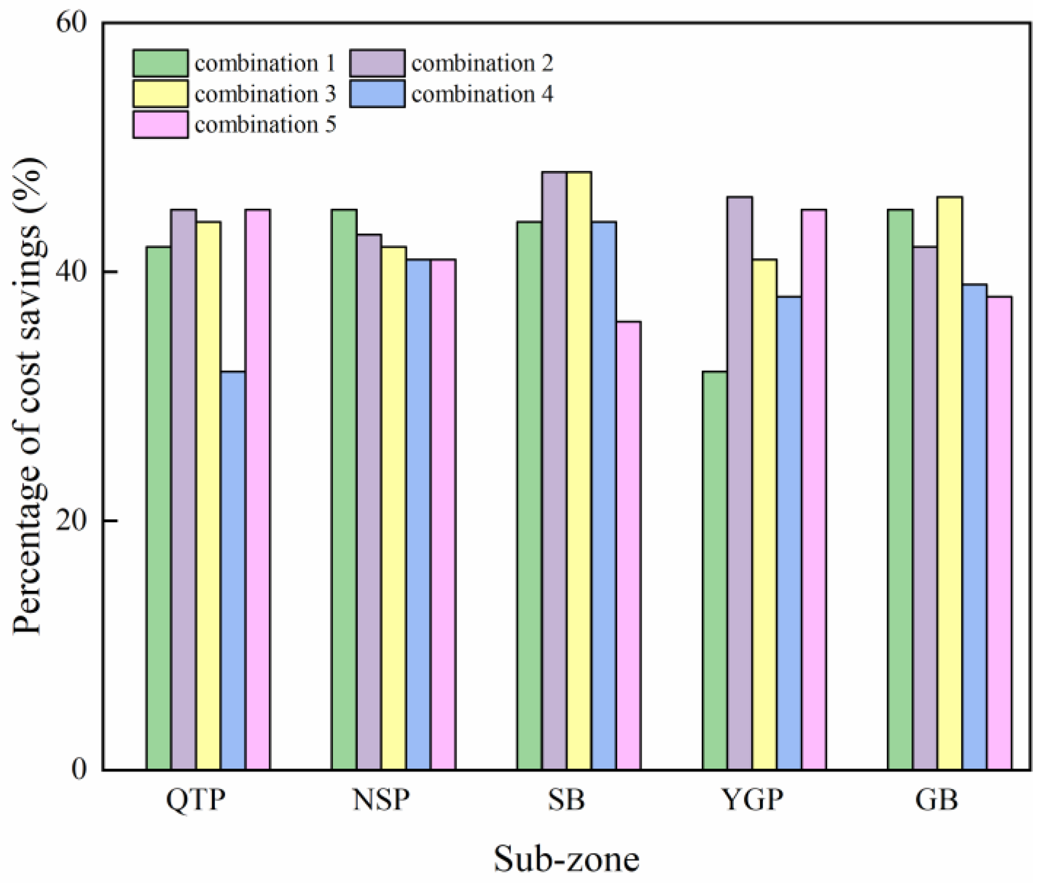
4.2. Combination of Input Parameters Decided Accuracy of ET0 Prediction Models

The combination of input parameters had an important impact on the prediction accuracy of the ELM model for estimating ET0. In present study, the accuracy of ELM increased with increasing quantity of input parameters, and the calculated results of ELM and GA-ELM with complete input parameters were in good agreement with those of the FAO-56 PM model. The results were generally in accordance with the previous results reported by Antonopoulos and Torres [37,42]. The more meteorological parameters were input, the more information was obtained for ET0 prediction, improving the prediction accuracy of machine learning models. Feng et al. [43] found that RF and GRNN models with complete parameters inputs of Tmax, Tmin, Tmean, RH, u2 and Rs obtained satisfactory results in ET0 prediction. Yu et al. [40] applied different combinations of Tmax, Tmin, u2, RH, and Rs to predict ET0 in the arid area Altay Prefecture, and the results confirmed that the ELM model with complete inputs exhibited the best prediction accuracy. Chia et al. [19] employed six input combinations to evaluate the accuracies of hybridized ELM models with Tmax, Tmin, Tmean, RH, u2 and Rs as input parameters accurately predicted ET0, and the prediction accuracy of ELM model decreased as with reducing input parameters. Generally, the more input parameters improved the ET0 prediction accuracy of machine learning model, but the contribution of meteorological parameters to the ET0 estimation was different.
The input combination strategy of meteorological data also affected the performance of machine learning models. Previous studies have shown that solar radiation and sunshine duration were important meteorological factors affecting ET0 in tropical and subtropical monsoon zones of China [4]. In the present study, the accuracy of models with radiation parameters was obviously higher than those only with temperature parameters. In addition, when same quantity of parameters was imputed, the performance of ELM and GA-ELM models with Rn inputted were slightly better than those with Rs in most sub-zones, indicating that Rn was a more influential factor in ET0 prediction in Southwest China. Feng et al. [8,43] also found that models employing Rn performed better than models employing Rs in SB. According to Irmak et al. [28], the prediction accuracy of the Rn-based model was better than the Rs-based model in humid climates. Nevertheless, the contribution of input parameter to the ET0 prediction varied in different zones in Southwest China. In the present study, models with Rs performed better than models with Rn in YGP. As a result of the changeable terrain and climate, as well as uneven radial distribution of solar radiation in YGP, Rs was the main meteorological factor affecting ET0 [44]. In fact, in actual observations, both Rs and Rn can be obtained by pyranometer of the meteorological observation station [45]. However, Rs and Rn are usually calculated by other meteorological parameters in areas lacking radiation observation. Rs can be calculated by extraterrestrial radiation and sunshine duration [46]. Rn is the difference between net shortwave radiation and net longwave radiation, and net shortwave radiation needs to be calculated by Rs [3]. ET0 was more susceptible to Rn in Southwest China, but Rs was easier to be obtained than Rn for ET0 prediction with acceptable accuracy. Therefore, Rs is a better choice as input parameter for ET0 estimation, especially in YGP.

4.3. GA Improved the Performance of ELM Models

It is well known that the prediction of the ELM model mainly depends on its kernel function. The internal parameters of ELM model are randomly initialized, which may generate non-optimal solutions and local optimum, affecting the performance of ELM model [41,47]. Therefore, applying an optimization algorithm to tune the parameters of machine learning models can improve the ET0 prediction accuracy of ELM. Zhu et al. [41] utilized a PSO algorithm to optimally determine the parameters of ELM model under limited inputs condition. The results showed that PSO-ELM model accurately predicted daily ET0 in Northwest China. Wu et al. [48] proposed three hybrid models for predicting daily ET0 in different climatic zones of China, and the results indicated that the biological heuristic algorithms effectively improved the performance of ELM model. The present study showed that GA effectively improved the performance of ELM in predicting ET0, which was in consistent with the above conclusions.
Previous studies showed that the quantity of hidden neurons was affected by the quantity of input parameters. Meanwhile, the computational cost of ELM was associated with the hidden neurons [49]. Optimization efficiency is a major factor for the computational cost of optimized ELM models [49]. In the context of this study, the task of GA was to search for the optimal hidden neurons for ELM model. To further evaluate the comprehensive performance of GA-ELM model, the averaged computational time of machine learning models with different inputs was recorded (Figure 9). In each sub-zone, the computational costs were significantly saved under each input combination. The averaged computational cost saving of combinations 1–5 (as seen from Table 2) were 42%, 45%, 44%, 39%, and 41%, respectively. The increased quantity of input parameters into ELM model improved the prediction accuracy of ET0 estimation but decreased optimization efficiency, which was in agreement with the conclusion of Chia et al. and Jose V. Frances-Villora [19,50]. The internal kernel function of ELM is too complex to determine in one time [17]. GA have strong global convergence ability and can neglect the information regarding the gradient [51], so the input weights and node thresholds of ELM could be optimized by GA. In conclusion, GA effectively saved computational cost of the ELM model and improved the prediction accuracy, which can be recommended to optimize the machine learning model for ET0 estimation.
However, this study only explored the accuracy and computational cost for the ET0 estimation of the ELM/GA-ELM model under different input combinations. Using different machine learning models to predict daily ET0 under limited meteorological data input, evaluating the potential of different machine learning models for ET0 prediction, and applying a variety of more advanced optimization algorithms to optimize ELM or other machine learning models to improve the accuracy of ET0 estimation will be important research aspects of ET0 prediction. In addition, the accuracy and computational cost of GA-ELM models for ET0 prediction in satellite-based ET retrievals should be further explored.

5. Conclusions

In the present study, ELM and GA-ELM models for ET0 estimation were developed based on daily meteorological data from 15 representative meteorological stations in Southwest China. The prediction accuracy of ELM and GA-ELM models with five inputs of meteorological data and five empirical models were evaluated based on the calculated ET0 from the PM model. The results showed that:
(1) GA-ELM models performed best in estimating ET0 in Southwest China, with R2 ranging 0.56–0.99 and RMSE ranging 0.033–0.771 mm·d−1, followed by ELM models, with R2 ranging 0.59–0.99, RMSE ranging 0.080–0.77 mm·d−1, and the empirical models performed worst, with R2 ranging 0.36–0.91, RMSE ranging 0.69–2.64 mm·d−1.
(2) The GA-ELM5 model performed best among the models with five input parameters (Tmax, Tmin, u2, RH, Rn/Rs), with R2 ranging 0.99–0.99, RMSE ranging 0.03–0.11 mm·d−1. The GA-ELM3 model performed best with input combinations of three parameters (Tmax, Tmin, Rn/Rs), with R2 ranging 0.79–0.99, RMSE ranging 0.15–0.65 mm·d−1. Regarding to the input combination of Tmax and Tmin, the GA-ELM1 model outperformed the ELM1 model, with R2 ranging 0.56–0.89, RMSE ranging 0.47–0.87 mm·d−1. Models involving Rn outperformed those involving Rs under the same input parameter quantity.
(3) GA-ELM5 model (Tmax, Tmin, u2, RH, Rn) could be recommended as the ET0 estimation model for Southwest China under complete meteorological data, with R2 ranging 0.9939–0.9996, RMSE ranging 0.03–0.11 mm·d−1. Considering that Rs is easier and cheaper to obtain than Rn, the GA-ELM2 model (Tmax, Tmin, Rs) was also acceptable to estimate daily ET0 in Southwest China with high accuracy under limited meteorological data conditions, with R2 ranging 0.78–0.99, RMSE ranging 0.14–0.67 mm·d−1.
This study can provide a reliable method for accurate prediction of daily ET0 in Southwest China under the condition of missing or limited meteorological parameters, and provide reference for optimizing ELM model or other machine learning models to predict ET0. In addition, applying multiple advanced optimization algorithms to optimize machine learning models to improve the estimation accuracy will become an important research direction for ET0 prediction.

Author Contributions

Q.L.: conceptualization, methodology, investigation, writing—original draft. Z.W.: formal analysis, investigation. N.C.: conceptualization, methodology, writing—review and editing, funding acquisition. W.Z.: writing—review and editing. Y.W.: resources, writing—review and editing. X.H.: writing—review and editing. D.G.: methodology. S.Z.: investigation, writing—review and editing. All authors have read and agreed to the published version of the manuscript.

Funding

This work was supported by the National Natural Science Foundation of China (51922072, 51779161) and the National Key Research and Development Program of China (No.2016YFC0400206).

Institutional Review Board Statement

Not applicable.

Informed Consent Statement

Not applicable.

Data Availability Statement

The meteorological data used in this study are available here: http://data.cma.cn, accessed on 1 November 2021.

Acknowledgments

The authors would like to thank the National Climatic Centre of the China Meteorological Administration for providing the climate database used in this study. Thanks also go to the reviewers and editors for thorough comments that really helped to improve the manuscript.

Conflicts of Interest

The authors declare no conflict of interest.

References

  1. Fan, J.; Wu, L.; Zhang, F.; Xiang, Y.; Zheng, J. Climate change effects on reference crop evapotranspiration across different climatic zones of China during 1956–2015. J. Hydrol. 2016, 542, 923–937. [Google Scholar] [CrossRef]
  2. Lai, C.; Chen, X.; Zhong, R.; Wang, Z. Implication of climate variable selections on the uncertainty of reference crop evapotranspiration projections propagated from climate variables projections under climate change. Agric. Water Manag. 2022, 259, 107273. [Google Scholar] [CrossRef]
  3. Allen, R.G.; Pereira, L.S.; Raes, D.; Smith, M. Crop Evapotranspiration-Guidelines for Computing Crop Water Requirements-FAO Irrigation and Drainage Paper 56; FAO: Rome, Italy, 1998.
  4. Fan, J.; Yue, W.; Wu, L.; Zhang, F.; Cai, H.; Wang, X.; Lu, X.; Xiang, Y. Evaluation of SVM, ELM and four tree-based ensemble models for predicting daily reference evapotranspiration using limited meteorological data in different climates of China. Agric. For. Meteorol. 2018, 263, 225–241. [Google Scholar] [CrossRef]
  5. Hargreaves, G.H.; Samani, Z.A. Reference Crop Evapotranspiration from Temperature. Appl. Eng. Agric. 1985, 1, 96–99. [Google Scholar] [CrossRef]
  6. Priestley, C.H.B.; Taylor, R.J. On the Assessment of Surface Heat Flux and Evaporation Using Large-Scale Parameters. Mon. Weather Rev. 1972, 100, 81–92. [Google Scholar] [CrossRef]
  7. Samani, Z. Estimating solar radiation and evapotranspiration using minimum climatological data. J. Irrig. Drain. Eng. 2000, 126, 265–267. [Google Scholar] [CrossRef]
  8. Feng, Y.; Cui, N.; Zhao, L.; Hu, X.; Gong, D. Comparison of ELM, GANN, WNN and empirical models for estimating reference evapotranspiration in humid region of Southwest China. J. Hydrol. 2016, 536, 376–383. [Google Scholar] [CrossRef]
  9. Ferreira, L.B.; da Cunha, F.F.; de Oliveira, R.A.; Filho, E.I.F. Estimation of reference evapotranspiration in Brazil with limited meteorological data using ANN and SVM–A new approach. J. Hydrol. 2019, 572, 556–570. [Google Scholar] [CrossRef]
  10. Balde, A.B.; Sow, A.; Muller, B.; Irmak, S.; N’Diaye, M.K.; Baboucarr, M.; Moukoumbi, Y.D.; Futakuchi, K.; Saito, K. Evaluation of sixteen reference evapotranspiration methods under sahelian conditions in the Senegal River Valley. J. Hydrol. Reg. Stud. 2015, 3, 139–159. [Google Scholar] [CrossRef] [Green Version]
  11. Zhang, Q.; Cui, N.; Feng, Y.; Gong, D.; Hu, X. Improvement of Makkink model for reference evapotranspiration estimation using temperature data in Northwest China. J. Hydrol. 2018, 566, 264–273. [Google Scholar] [CrossRef]
  12. Kisi, O.; Alizamir, M. Modelling reference evapotranspiration using a new wavelet conjunction heuristic method: Wavelet extreme learning machine vs. wavelet neural networks. Agric. For. Meteorol. 2018, 263, 41–48. [Google Scholar] [CrossRef]
  13. Mehdizadeh, S. Estimation of daily reference evapotranspiration (ETo) using artificial intelligence methods: Offering a new approach for lagged ETo data-based modeling. J. Hydrol. 2018, 559, 794–812. [Google Scholar] [CrossRef]
  14. Yassin, M.A.; Alazba, A.; Mattar, M.A. Artificial neural networks versus gene expression programming for estimating reference evapotranspiration in arid climate. Agric. Water Manag. 2016, 163, 110–124. [Google Scholar] [CrossRef]
  15. Tabari, H.; Kisi, O.; Ezani, A.; Talaee, P.H. SVM, ANFIS, regression and climate based models for reference evapotranspiration modeling using limited climatic data in a semi-arid highland environment. J. Hydrol. 2012, 444, 78–89. [Google Scholar] [CrossRef]
  16. Chen, H.; Huang, J.J.; McBean, E. Partitioning of daily evapotranspiration using a modified shuttleworth-wallace model, random Forest and support vector regression, for a cabbage farmland. Agric. Water Manag. 2019, 228, 105923. [Google Scholar] [CrossRef]
  17. Huang, G.-B.; Zhu, Q.-Y.; Siew, C.-K. Extreme learning machine: Theory and applications. Neurocomputing 2006, 70, 489–501. [Google Scholar] [CrossRef]
  18. Abdullah, S.S.; Malek, M.; Abdullah, N.S.; Kisi, O.; Yap, K.S. Extreme Learning Machines: A new approach for prediction of reference evapotranspiration. J. Hydrol. 2015, 527, 184–195. [Google Scholar] [CrossRef]
  19. Chia, M.Y.; Huang, Y.F.; Koo, C.H. Swarm-based optimization as stochastic training strategy for estimation of reference evapotranspiration using extreme learning machine. Agric. Water Manag. 2020, 243, 106447. [Google Scholar] [CrossRef]
  20. Wu, L.; Zhou, H.; Ma, X.; Fan, J.; Zhang, F. Daily reference evapotranspiration prediction based on hybridized extreme learning machine model with bio-inspired optimization algorithms: Application in contrasting climates of China. J. Hydrol. 2019, 577, 123960. [Google Scholar] [CrossRef]
  21. Zhao, L.; Zhao, X.; Zhou, H.; Wang, X.; Xing, X. Prediction model for daily reference crop evapotranspiration based on hybrid algorithm and principal components analysis in Southwest China. Comput. Electron. Agric. 2021, 190, 106424. [Google Scholar] [CrossRef]
  22. Wang, P.; Wu, X.; Hao, Y.; Wu, C.; Zhang, J. Is Southwest China drying or wetting? Spatiotemporal patterns and potential causes. Theor. Appl. Climatol. 2019, 139, 1–15. [Google Scholar] [CrossRef]
  23. Hassan, M.A.; Khalil, A.; Kaseb, S.; Kassem, M. Exploring the potential of tree-based ensemble methods in solar radiation modeling. Appl. Energ. 2017, 203, 897–916. [Google Scholar] [CrossRef]
  24. Wu, Z.; Cui, N.; Zhu, B.; Zhao, L.; Wang, X.; Hu, X.; Wang, Y.; Zhu, S. Improved Hargreaves Model Based on Multiple Intelligent Optimization Algorithms to Estimate Reference Crop Evapotranspiration in Humid Areas of Southwest China. Atmos.-Basel 2021, 12, 15. [Google Scholar] [CrossRef]
  25. Zeng, Z.; Wu, W.; Zhou, Y.; Li, Z.; Hou, M.; Huang, H. Changes in Reference Evapotranspiration over Southwest China during 1960–2018: Attributions and Implications for Drought. Atmos.-Basel 2019, 10, 705. [Google Scholar] [CrossRef] [Green Version]
  26. Makkink, G.F. Testing the Penman Formula by Means of Lysimeters. J. Inst. Water Eng. 1957, 11, 277–288. [Google Scholar]
  27. Tabari, H.; Grismer, M.E.; Trajkovic, S. Comparative analysis of 31 reference evapotranspiration methods under humid conditions. Irrig. Sci. 2013, 31, 107–117. [Google Scholar] [CrossRef]
  28. Irmak, S.; Irmak, A.; Allen, R.G.; Jones, J.W. Solar and Net Radiation-Based Equations to Estimate Reference Evapotranspiration in Humid Climates. J. Irrig. Drain. Eng. 2003, 129, 336–347. [Google Scholar] [CrossRef]
  29. Holland, J.H. Adaptation in Natural and Artificial Systems; University of Michigan Press: Ann Arbor, MI, USA, 1975. [Google Scholar]
  30. Liu, W.; Chung, C.E. Enhancing the Predicting Accuracy of the Water Stage Using a Physical-Based Model and an Artificial Neural Network-Genetic Algorithm in a River System. Water-Sui. 2014, 6, 1642–1661. [Google Scholar] [CrossRef] [Green Version]
  31. Sharma, G.; Singh, A.; Jain, S. A hybrid deep neural network approach to estimate reference evapotranspiration using limited climate data. Neural Comput. Appl. 2021, 34, 4013–4032. [Google Scholar] [CrossRef]
  32. Mokhtar, A.; He, H.; Alsafadi, K.; Li, Y.; Zhao, H.; Keo, S.; Bai, C.; Abuarab, M.; Zhang, C.; Elbagoury, K.; et al. Evapotranspiration as a response to climate variability and ecosystem changes in southwest, China. Environ. Earth Sci. 2020, 79, 1–21. [Google Scholar] [CrossRef]
  33. Koca, A.; Oztop, H.F.; Varol, Y.; Koca, G.O. Estimation of solar radiation using artificial neural networks with different input parameters for Mediterranean region of Anatolia in Turkey. Expert Syst. Appl. 2011, 38, 8756–8762. [Google Scholar] [CrossRef]
  34. Zhang, Y.; Cui, N.; Feng, Y.; Gong, D.; Hu, X. Comparison of BP, PSO-BP and statistical models for predicting daily global solar radiation in arid Northwest China. Comput. Electron. Agric. 2019, 164, 104905. [Google Scholar] [CrossRef]
  35. Citakoglu, H. Comparison of artificial intelligence techniques via empirical equations for prediction of solar radiation. Comput. Electron. Agric. 2015, 118, 28–37. [Google Scholar] [CrossRef]
  36. Feng, Y.; Jia, Y.; Zhang, Q.; Gong, D.; Cui, N. National-scale assessment of pan evaporation models across different climatic zones of China. J. Hydrol. 2018, 564, 314–328. [Google Scholar] [CrossRef]
  37. Yang, Y.; Chen, R.; Han, C.; Liu, Z.; Wang, X. Optimal Selection of Empirical Reference Evapotranspiration Method in 36 Different Agricultural Zones of China. Agronomy 2022, 12, 31. [Google Scholar] [CrossRef]
  38. Wang, L.; Kisi, O.; Zounemat-Kermani, M.; Li, H. Pan evaporation modeling using six different heuristic computing methods in different climates of China. J. Hydrol. 2017, 544, 407–427. [Google Scholar] [CrossRef]
  39. Yin, Z.; Feng, Q.; Yang, L.; Deo, R.; Wen, X.; Si, J.; Xiao, S. Future Projection with an Extreme-Learning Machine and Support Vector Regression of Reference Evapotranspiration in a Mountainous Inland Watershed in North-West China. Water-Sui. 2017, 9, 880. [Google Scholar] [CrossRef] [Green Version]
  40. Yu, H.; Wen, X.; Li, B.; Yang, Z.; Wu, M.; Ma, Y. Uncertainty analysis of artificial intelligence modeling daily reference evapotranspiration in the northwest end of China. Comput. Electron. Agric. 2020, 176, 105653. [Google Scholar] [CrossRef]
  41. Zhu, B.; Feng, Y.; Gong, D.; Jiang, S.; Zhao, L.; Cui, N. Hybrid particle swarm optimization with extreme learning machine for daily reference evapotranspiration prediction from limited climatic data. Comput. Electron. Agric. 2020, 173, 105430. [Google Scholar] [CrossRef]
  42. Antonopoulos, V.Z.; Antonopoulos, A.V. Daily reference evapotranspiration estimates by artificial neural networks technique and empirical equations using limited input climate variables. Comput. Electron. Agric. 2017, 132, 86–96. [Google Scholar] [CrossRef]
  43. Feng, Y.; Jia, Y.; Cui, N.; Zhao, L.; Li, C.; Gong, D. Calibration of Hargreaves model for reference evapotranspiration estimation in Sichuan basin of southwest China. Agric. Water Manag. 2017, 181, 1–9. [Google Scholar] [CrossRef]
  44. Zhao, R.; Wang, K.; Wu, G.; Zhou, C. Temperature annual cycle variations and responses to surface solar radiation in China between 1960 and 2016. Int. J. Climatol. 2021, 41, E2959–E2978. [Google Scholar] [CrossRef]
  45. Besharat, F.; Dehghan, A.A.; Faghih, A.R. Empirical models for estimating global solar radiation: A review and case study. Renew. Sustain. Energy Rev. 2013, 21, 798–821. [Google Scholar] [CrossRef]
  46. Ågnström, A. Solar and Terrestrial Radiation. 19. Mon. Weather Rev. 1924, 52, 83. [Google Scholar] [CrossRef]
  47. Mohapatra, P.; Chakravarty, S.; Dash, P.K. An improved cuckoo search based extreme learning machine for medical data classification. Swarm Evol. Comput. 2015, 24, 25–49. [Google Scholar] [CrossRef]
  48. Wu, Z.; Cui, N.; Hu, X.; Gong, D.; Wang, Y.; Feng, Y.; Jiang, S.; Lv, M.; Han, L.; Xing, L.; et al. Optimization of extreme learning machine model with biological heuristic algorithms to estimate daily reference crop evapotranspiration in different climatic regions of China. J. Hydrol. 2021, 603, 127028. [Google Scholar] [CrossRef]
  49. Tejada, A.T.; Ella, V.B.; Lampayan, R.M.; Reaño, C.E. Modeling Reference Crop Evapotranspiration Using Support Vector Machine (SVM) and Extreme Learning Machine (ELM) in Region IV-A, Philippines. Water-Sui. 2022, 14, 754. [Google Scholar] [CrossRef]
  50. Rosado-Muñoz, A.; Frances-Villora, J.V. Hardware implementation of real-time Extreme Learning Machine in FPGA: Analysis of precision, resource occupation and performance R. Comput. Electr. Eng. 2016, 51, 139–156. [Google Scholar]
  51. Whitley, D. A Genetic algorithm tutorial. Stat. Comput. 1994, 4, 65–85. [Google Scholar] [CrossRef]
Figure 1. Geographic locations of the representative meteorological stations and five zones in Southwest China.
Atmosphere 13 00971 g001
Figure 2. Topological structure of extreme learning machine.
Atmosphere 13 00971 g002
Figure 3. The flowchart of GA-ELM.
Atmosphere 13 00971 g003
Figure 4. R2 of meteorological parameters for ET0 estimated using the Penman–Monteith model.
Atmosphere 13 00971 g004
Figure 5. Boxplots of statistical indicators for each daily ET0 prediction model in Southwest China. Blue: ELM models; green: GA-ELM models; yellow: empirical models.
Atmosphere 13 00971 g005
Figure 6. Scatter plots of predicted ET0 values using ELM models against their corresponding FAO56-PM values during testing in Southwest China. (Note: the fine line represents 1:1 line).
Atmosphere 13 00971 g006
Figure 7. Scatter plots of predicted ET0 values using GA-ELM models against their corresponding FAO56-PM values during testing in Southwest China. (Note: the fine line represents 1:1 line).
Atmosphere 13 00971 g007
Figure 8. GPI ranking of each model at all stations.
Atmosphere 13 00971 g008
Figure 9. Percentage of computational cost saving for GA-ELM models under different input combinations.
Atmosphere 13 00971 g009
Table 1. Annual means of the main meteorological parameters at each station during 1992–2016.
ZoneStationLon
(°)
Lat
(°)
H
(m)
Tmax
(°C)
Tmin
(°C)
RH
(%)
u2
(m·s−1)
Rs
(MJ·m−2·d−1)
Rn
(MJ·m−2·d−1)
QTPShiquanhe80.0532.3042789.02−5.98311.8920.0311.54
Gaize84.2532.0944148.90−7.19342.5118.9711.04
Anduo91.0632.2152005.25−8.04532.5017.5010.40
Zedang91.4629.16356017.282.93421.5118.2610.41
NSPHongyuan102.3332.48349110.72−4.57701.7215.679.29
Ganzi10031.37339314.700.11561.3216.449.54
Zuogong97.529.40378013.26−1.10551.0015.913.15
SBBazhong106.4631.5241721.7213.71770.6512.777.60
Dazu105.4229.4239421.4914.28832.611.527.17
YGPDali100.1125.42199021.4910.66671.7616.3110.65
Huize103.1526.24218819.339.02691.9216.6310.84
Meitan107.2827.4679219.6812.51801.3211.958.29
Yuanjiang101.5923.3640031.0119.45671.6117.0611.43
GBLaibin109.0923.469625.7218.15751.1213.648.12
Bama107.1524.0825426.1517.36800.9513.878.25
Table 2. Summary of the input data for each ET0 model.
Extreme Learning MachineExtreme Learning Machine Optimized
by Genetic Algorithm
Input DataEmpirical Models
ELM1GA-ELM1Tmax, TminRomanenko (Ro)
ELM2GA-ELM2Tmax, Tmin, RsMakkink (MK)
ELM3GA-ELM3Tmax, Tmin, RnTabari (TAB)
ELM4GA-ELM4Tmax, Tmin, Rs, u2, RHIrmak–Allen (IA)
ELM5GA-ELM5Tmax, Tmin, Rn, u2, RHPriestley–Taylor (PT)
Table 3. Statistical performance of ET0 models in sub-zones.
Sub-zoneModelTrainingTesting
R2RMSE
(mm·d−1)
RRMSEMAE
(mm·d−1)
GPIRankR2RMSE
(mm·d−1)
RRMSEMAE
(mm·d−1)
GPIRank
QTPELM10.94 0.62 0.17 0.49 −0.40 100.85 0.60 0.15 0.48 −0.50 10
ELM20.97 0.41 0.11 0.33 0.06 70.93 0.40 0.10 0.31 0.00 8
ELM30.98 0.40 0.11 0.31 0.10 60.940.40 0.10 0.31 0.02 6
ELM40.99 0.20 0.20 0.16 0.38 40.98 0.21 0.05 0.16 0.45 4
ELM50.99 0.15 0.04 0.11 0.63 30.99 0.12 0.03 0.09 0.63 2
GA-ELM10.95 0.62 0.17 0.49 −0.39 80.86 0.61 0.15 0.48 −0.50 9
GA-ELM20.97 0.42 0.11 0.33 0.06 90.940.40 0.10 0.31 0.01 7
GA-ELM30.98 0.40 0.11 0.31 0.10 50.940.39 0.10 0.30 0.03 5
GA-ELM40.990.14 0.04 0.11 0.64 20.99 0.15 0.04 0.11 0.58 3
GA-ELM50.990.05 0.01 0.04 0.83 10.99 0.07 0.02 0.04 0.75 1
Ro//////0.69 1.260.33 1.05 −2.06 13
MK//////0.91 1.33 0.34 1.23 −2.11 14
TAB//////0.91 1.50 0.49 1.84 −3.03 15
IA//////0.83 0.74 0.19 0.61 −0.83 12
PT//////0.91 0.72 0.18 0.59 −0.70 11
NSPELM10.92 0.61 0.19 0.50 −0.47 100.76 0.60 0.18 0.48 −0.57 10
ELM20.96 0.420.13 0.33 0.00 80.90 0.39 0.12 0.31 0.00 8
ELM30.96 0.41 0.12 0.32 0.03 60.91 0.38 0.11 0.30 0.04 6
ELM40.99 0.17 0.05 0.13 0.55 40.98 0.17 0.05 0.13 0.55 4
ELM50.99 0.10 0.03 0.07 0.71 20.99 0.09 0.03 0.07 0.72 2
GA-ELM10.92 0.61 0.19 0.50 −0.47 90.77 0.60 0.18 0.47 −0.56 9
GA-ELM20.96 0.42 0.13 0.32 0.00 70.90 0.3 0.11 0.31 0.01 7
GA-ELM30.96 0.40 0.12 0.31 0.03 50.91 0.38 0.11 0.29 0.05 5
GA-ELM40.99 0.14 0.04 0.11 0.61 30.99 0.14 0.04 0.11 0.623
GA-ELM50.99 0.03 0.01 0.03 0.84 10.999 0.03 0.01 0.03 0.84 1
Ro//////0.59 1.26 0.37 1.07 −2.20 13
MK//////0.74 1.52 0.42 1.31 −2.61 14
TAB//////0.57 1.97 0.55 1.83 −3.86 15
IA//////0.74 0.81 0.22 0.62 −0.99 11
PT//////0.80 0.930.26 0.72 −1.19 12
SBELM10.85 0.70 0.23 0.55−0.36 100.81 0.75 0.22 0.56 −0.45 11
ELM20.92 0.56 0.18 0.41 0.0170.89 0.57 0.17 0.42 0.00 8
ELM30.94 0.54 0.18 0.39 0.08 50.90 0.56 0.16 0.420.03 6
ELM40.99 0.18 0.06 0.14 0.88 40.99 0.180.05 0.13 0.92 4
ELM50.99 0.07 0.02 0.06 1.1020.99 0.08 0.03 0.06 1.10 2
GA-ELM10.87 0.70 0.23 0.55 −0.35 90.81 0.74 0.22 0.56 −0.4410
GA-ELM20.92 0.57 0.19 0.42 0.01 80.89 0.57 0.17 0.42 0.01 7
GA-ELM30.93 0.54 0.18 0.40 0.07 60.90 0.56 0.16 0.41 0.03 5
GA-ELM40.99 0.14 0.04 0.10 0.97 30.99 0.13 0.04 0.10 0.99 3
GA-ELM50.99 0.04 0.01 0.03 1.18 10.99 0.04 0.01 0.03 2.001
Ro//////0.69 1.32 0.39 1.09 −1.8 14
MK//////0.85 1.49 0.44 1.36 −2.2 15
TAB//////0.89 1.26 0.37 1.13 −1.60 13
IA//////0.880.69 0.20 0.52 −0.26 9
PT//////0.89 0.88 0.26 0.73 −0.71 12
YGPELM10.80 0.76 0.23 0.58 −0.93 100.71 0.76 0.22 0.58 −0.95 11
ELM20.95 0.35 0.10 0.250.10 60.93 0.36 0.10 0.26 0.13 6
ELM30.93 0.39 0.11 0.27 0.00 80.91 0.41 0.12 0.30 0.00 8
ELM40.990.14 0.04 0.11 0.54 40.99 0.15 0.04 0.11 0.60 4
ELM50.99 0.10 0.03 0.07 0.64 20.99 0.11 0.03 0.08 0.68 2
GA-ELM10.80 0.75 0.23 0.58 −0.92 90.71 0.76 0.22 0.58 −0.94 10
GA-ELM20.95 0.34 0.10 0.25 0.10 50.93 0.35 0.10 0.26 0.14 5
GA-ELM30.94 0.38 0.11 0.270.01 70.92 0.39 0.11 0.28 0.04 7
GA-ELM40.99 0.12 0.04 0.09 0.59 30.99 0.11 0.03 0.09 0.67 3
GA-ELM50.99 0.07 0.02 0.05 0.71 10.99 0.07 0.02 0.05 0.76 1
Ro//////0.77 1.17 0.33 0.92 −1.73 15
MK//////0.88 0.94 0.27 0.78 −1.20 13
TAB//////0.85 0.96 0.28 0.75 −1.23 14
IA//////0.85 0.81 0.25 0.72−1.02 12
PT//////0.84 0.73 0.22 0.60 −0.80 9
GBELM10.59 0.77 0.20 0.61 −0.63 100.73 0.77 0.19 0.60 −0.40 10
ELM20.87 0.60 0.15 0.46 0.01 60.83 0.63 0.15 0.48 0.00 8
ELM30.88 0.61 0.16 0.460.01 70.83 0.63 0.15 0.47 0.01 6
ELM40.99 0.18 0.05 0.14 0.99 40.98 0.18 0.04 0.13 1.06 4
ELM50.99 0.11 0.03 0.07 1.15 20.99 0.10 0.030.07 1.22 2
GA-ELM10.56 0.62 0.20 0.61−0.50 90.73 0.77 0.19 0.59 −0.39 9
GA-ELM20.89 0.60 0.15 0.46 0.03 50.83 0.63 0.15 0.48 0.00 7
GA-ELM30.87 0.61 0.15 0.470.01 80.84 0.62 0.15 0.47 0.02 5
GA-ELM40.99 0.150.04 0.12 1.05 30.99 0.15 0.04 0.11 1.12 3
GA-ELM50.99 0.03 0.01 0.03 1.29 10.99 0.03 0.01 0.02 1.36 1
Ro//////0.36 1.61 0.39 1.28 −2.48 13
MK//////0.80 1.880.45 1.76 −2.87 14
TAB//////0.821.54 0.37 1.41 −2.08 12
IA//////0.82 1.01 0.24 0.81 −0.82 11
PT//////0.832.64 0.63 2.24 −4.25 15
Table 4. Statistical performance of ET0 models in Southwest China.
ModelTrainingTesting
R2RMSE
(mm·d−1)
RRMSEMAEGPIRankR2RMSE
(mm·d−1)
RRMSEMAEGPIRank
ELM10.9409 0.4093 0.1282 0.3425 0.2608100.7311 0.7744 0.1873 0.5979 −0.3987 10
ELM20.9887 0.1944 0.0604 0.1520 0.231680.8279 0.6285 0.1520 0.4772 0.0000 8
ELM30.9874 0.1724 0.0536 0.13160.193460.8344 0.6263 0.1514 0.4742 0.0124 6
ELM40.9957 0.1077 0.0335 0.0861 0.187840.9843 0.1769 0.0428 0.1321 1.0623 4
ELM50.9977 0.0886 0.0275 0.0694 0.054120.9947 0.1034 0.0251 0.0720 1.2241 2
GA-ELM10.9450 0.4080 0.1278 0.3340 0.049290.7325 0.7707 0.1863 0.5935 −0.3882 9
GA-ELM20.9886 0.1898 0.0590 0.1476 0.011670.8288 0.6267 0.1516 0.4760 0.0043 7
GA-ELM30.9905 0.1716 0.0534 0.1308 0.001350.8359 0.6238 0.1508 0.4704 0.0207 5
GA-ELM40.9965 0.1053 0.0327 0.0845 −0.505430.9892 0.1460 0.0353 0.1143 1.1235 3
GA-ELM50.9985 0.0746 0.0232 0.0593 −0.519710.9995 0.0326 0.0079 0.0244 1.3645 1
Ro//////0.3605 1.6057 0.3875 1.2791 −2.4820 13
MK//////0.7965 1.8755 0.4532 1.7643 −2.8667 14
TAB//////0.8177 1.5410 0.3722 1.4144 −2.0800 12
IA//////0.8212 1.0084 0.2437 0.8147 −0.8158 11
PT//////0.8266 2.6417 0.6319 2.2367 −4.2538 15
Publisher’s Note: MDPI stays neutral with regard to jurisdictional claims in published maps and institutional affiliations.

