
Comparison of the Impact of Ship Emissions in Northern Europe and Eastern China

 , , ,
, , ,
Abstract
:1. Introduction
2. Materials and Methods
2.1. Model Simulations
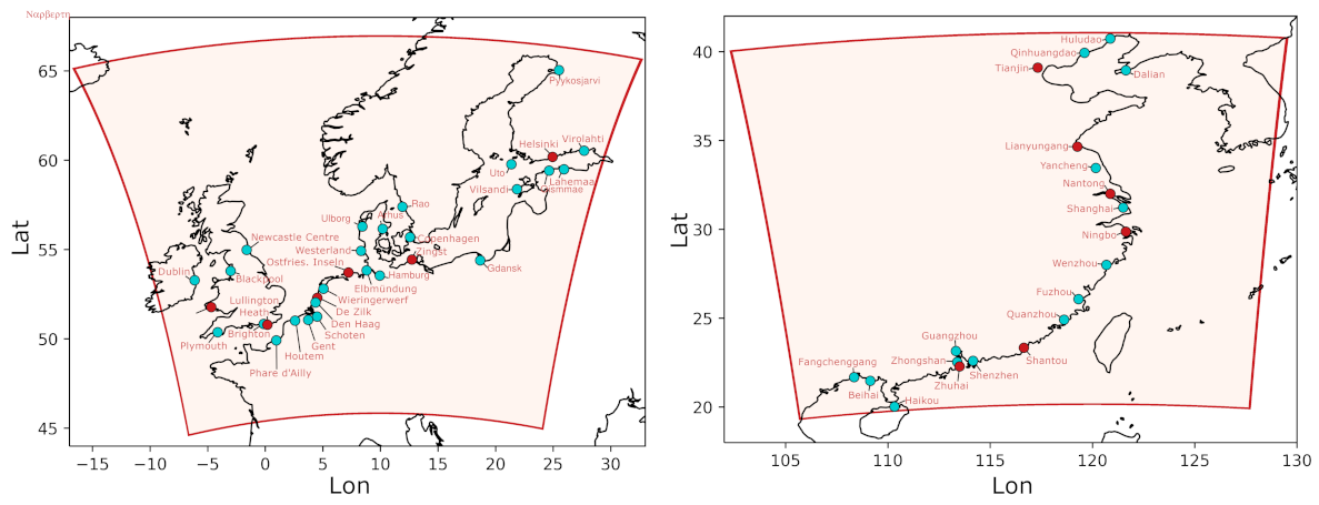
2.1.1. Regions of Interest
2.1.2. Chemical Transport Model CMAQ-Setup and Forcing
2.1.3. Meteorological Forcing
2.2. Emissions Data
2.2.1. Anthropogenic Land-Based Emissions for Europe
2.2.2. Anthropogenic Land-Based Emissions for China
2.2.3. Biogenic Emissions
2.2.4. Ship Emissions in Northern Europe
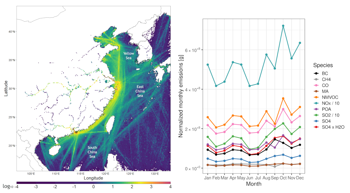
2.2.5. Ship Emissions in China
3. Assessment of the Model Performance
4. Results and Discussion
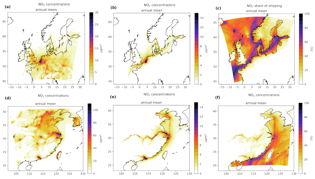
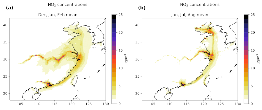
4.1. NO2
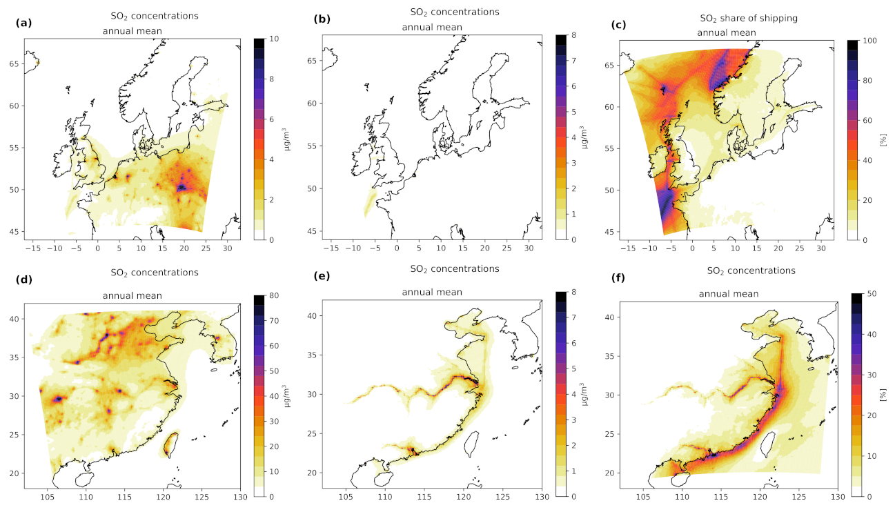
4.2. SO2
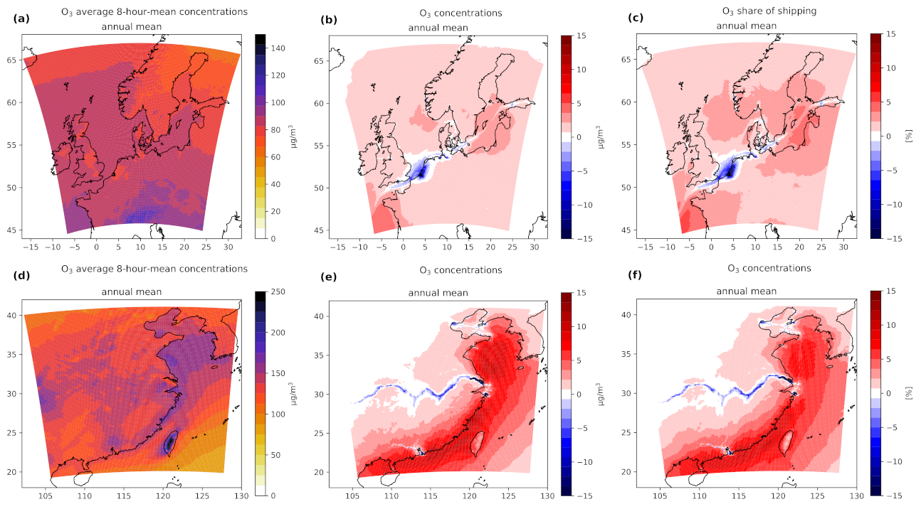
4.3. Ozone
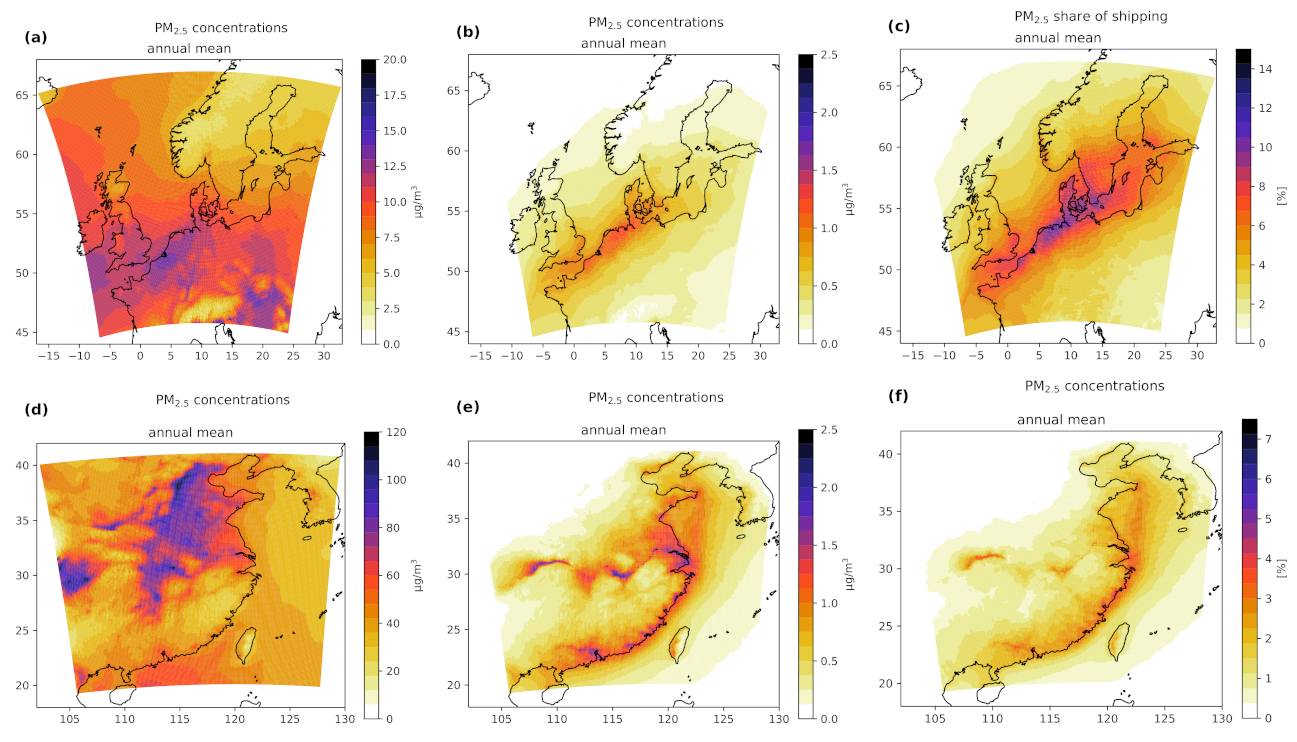
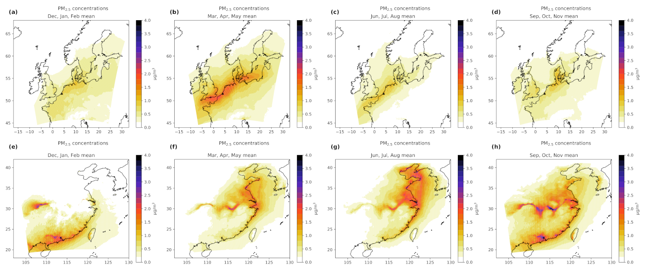
4.4. Fine Particulate Matter (PM2.5)
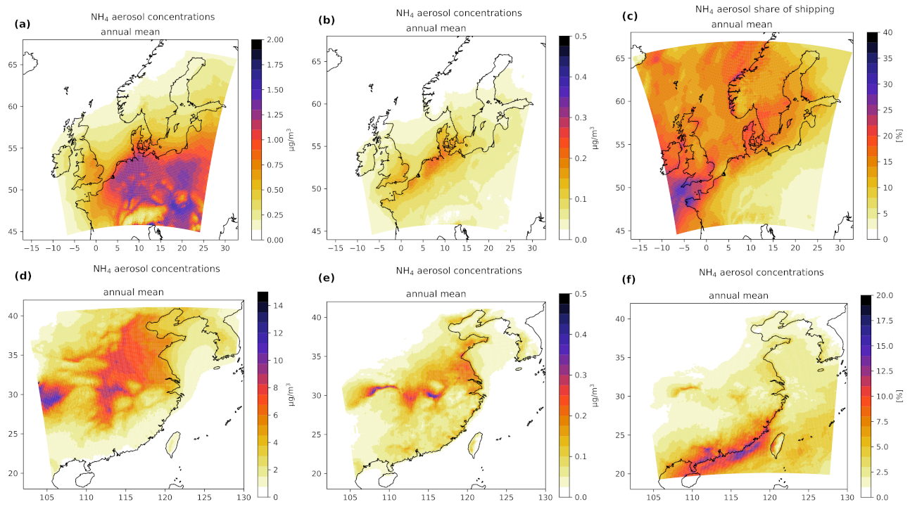
4.4.1. Ammonium (NH4)
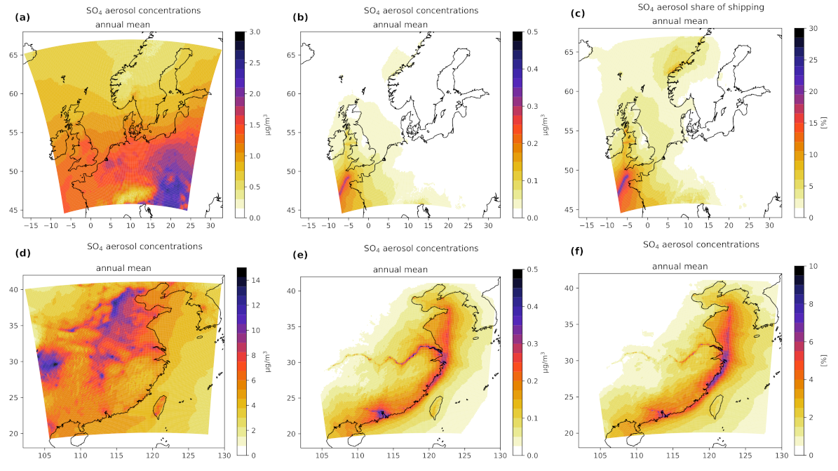
4.4.2. Sulfate (SO4)
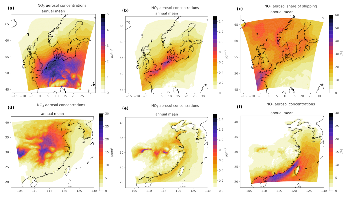
4.4.3. Nitrate (NO3)
5. Conclusions
Supplementary Materials
Author Contributions
Funding
Institutional Review Board Statement
Informed Consent Statement
Data Availability Statement
Conflicts of Interest
Abbreviations
| AIS | Automatic Identification System |
| AQER | Air Quality e-Reporting |
| BC | Black Carbon |
| BSH | German Federal Office for Sea Shipping and Hydrography |
| CAMS | Copernicus Atmosphere Monitoring Service |
| CMAQ | Community Multi-scale Air Quality model |
| CNC12 | Descriptor for the domain located in China |
| CNSS | Clean North Sea Shipping |
| COSMOS-CLM | Consortium for Small Scale Modelling in Climate Mode |
| DECA | Domestic Emission Control Area |
| ECA | Emission Control Area |
| ECCAD | Emissions of atmospheric Compounds and Compilation of Ancillary Data |
| ECMWF | European Centre for Medium-Range Weather Forecasts |
| EDGAR | Emissions Database for Global Atmospheric Research |
| EF | Emission Factor |
| EI | Emission Inventory |
| EMSA | European Maritime Safety Agency |
| FMI | Finnish Meteorological Institute |
| GNFR | Guidelines for reporting emissions and projections data Nomenclature For Reporting |
| HiMEMO | Highly Modular Emission Model |
| IMO | International Maritime Organization |
| IFS | Integrated Forecast System |
| IPCC | Intergovernmental Panel on Climate Change |
| LAI | Leaf Area Index |
| LYP | Lower Yangtze Plain |
| MA | Mineral Ash |
| MARPOL | International Convention for Prevention of Marine Pollution For Ships |
| MARS | Meteorological Archival and Retrieval System |
| MEGAN | Model of Emissions of Gases and Aerosols from Nature |
| MEIC | Multiresolution Emission Inventory for China |
| MoSES | Modular Ship Emission modeling System |
| NCP | North China Plain |
| NECA | Nitrogen Emission Control Area |
| NMB | Normalized Mean Bias |
| NMVOC | Nonmethane Organic Volatile Compounds |
| OC | Organic Compounds |
| PM | Particulate Matter |
| POA | Primary Organic Aerosol |
| PRD | Pearl River Delta |
| RCEP | Regional Comprehensive Economic Partnership |
| SC12NSBS | Descriptor for the domain located in northern Europe |
| SECA | Sulfur Emission Control Area |
| SHEBA | Sustainable Shipping and the Environment of the Baltic Sea Region |
| SNAP | Selected Nomenclature for Air Pollution |
| STEAM | Ship Traffic Emissions Assessment Model |
| TEU | Twenty-foot Equivalent Unit |
| TNO | The Netherlands Organisation for Applied Scientific Research |
| VOC | Volatile Organic Compounds |
| YRD | Yangtze River Delta |
Appendix A. Model Performance Data

| NO2 | SO2 | O3 8-h Mean | PM2.5 | |||||
|---|---|---|---|---|---|---|---|---|
| Station | Meanmodel | Meanmeas | Meanmodel | Meanmeas | Meanmodel | Meanmeas | Meanmodel | Meanmeas |
| Oismäe | — | — | ||||||
| Phare d’Ailly | — | — | — | — | — | — | ||
| Schoten | — | — | ||||||
| Utö | ||||||||
| Newcastle | — | — | ||||||
| Århus | — | — | — | — | ||||
| Westerland | — | — | ||||||
| De Zilk | ||||||||
| Den Haag | — | — | — | — | ||||
| Wieringerwerf | — | — | ||||||
| Pyykösjärvi | — | — | — | — | ||||
| Råö | — | — | — | — | — | — | ||
| Brighton | — | — | — | — | ||||
| Plymouth | — | — | ||||||
| Narberth | — | — | ||||||
| Blackpool | — | — | ||||||
| Dublin | — | — | — | — | — | — | ||
| Hamburg | — | — | — | — | ||||
| Lahemaa | — | — | ||||||
| Ostfries. Inseln | — | — | ||||||
| Elbmündung | — | — | — | — | ||||
| Virolahti | ||||||||
| Vilsandi | — | — | ||||||
| Copenhagen | — | — | — | — | ||||
| Ulborg | — | — | — | — | ||||
| Kallio | ||||||||
| Houtem | ||||||||
| Gent | ||||||||
| Lullington Heath | — | — | ||||||
| Zingst | — | — | ||||||
| Gdańsk Nowy Port | — | — | — | — | ||||
| Mean NMBpos | ||||||||
| Mean NMBneg | n.a. | |||||||
| Mean Corr. | ||||||||
| NO2 | SO2 | O3 8-h Mean | ||||||
|---|---|---|---|---|---|---|---|---|
| Station | Meanmodel | Meanmeas | Meanmodel | Meanmeas | Meanmodel | Meanmeas | Meanmodel | Meanmeas |
| Dalian | ||||||||
| Huludao | ||||||||
| Qinhuangdao | ||||||||
| Tianjin | ||||||||
| Lianyungang | ||||||||
| Yancheng | ||||||||
| Nantong | ||||||||
| Shanghai | ||||||||
| Ningbo | ||||||||
| Wenzhou | ||||||||
| Fuzhou | ||||||||
| Quanzhou | ||||||||
| Shantou | ||||||||
| Shenzhen | ||||||||
| Guangzhou | ||||||||
| Zhongshan | ||||||||
| Zhuhai | ||||||||
| Haikou | ||||||||
| Beihai | ||||||||
| Fangchenggang | ||||||||
| Mean, NMBpos | ||||||||
| Mean, NMBneg | ||||||||
| Mean Corr. | ||||||||
References
- UNCTAD. Review of Maritime Transport 2020; Technical Report; United Nations Conference on Trade and Development: Geneva, Switzerland, 2020. [Google Scholar]
- IMO. Second IMO Greenhouse Gas Study 2009; Technical Report; International Maritime Organisation: London, UK, 2009. [Google Scholar]
- IMO. Third IMO Greenhouse Gas Study 2014; Technical Report; IMO: London, UK, 2014. [Google Scholar] [CrossRef] [Green Version]
- Corbett, J.J.; Winebrake, J.J.; Green, E.H.; Kasibhatla, P.; Eyring, V.; Lauer, A. Mortality from ship emissions: A global assessment. Environ. Sci. Technol. 2007, 41, 8512–8518. [Google Scholar] [CrossRef] [PubMed]
- Dalsøren, S.B.; Eide, M.S.; Endresen, O.; Mjelde, A.; Gravir, G.; Isaksen, I.S. Update on emissions and environmental impacts from the international fleet of ships: The contribution from major ship types and ports. Atmos. Chem. Phys. 2009, 9, 2171–2194. [Google Scholar] [CrossRef] [Green Version]
- Liu, H.; Fu, M.; Jin, X.; Shang, Y.; Shindell, D.; Faluvegi, G.; Shindell, C.; He, K. Health and climate impacts of ocean-going vessels in East Asia. Nat. Clim. Chang. 2016, 6, 1037–1041. [Google Scholar] [CrossRef]
- Sofiev, M.; Winebrake, J.J.; Johansson, L.; Carr, E.W.; Prank, M.; Soares, J.; Vira, J.; Kouznetsov, R.; Jalkanen, J.P.; Corbett, J.J. Cleaner fuels for ships provide public health benefits with climate tradeoffs. Nat. Commun. 2018, 9, 1–12. [Google Scholar] [CrossRef] [PubMed] [Green Version]
- Hassellöv, I.M.; Turner, D.R.; Lauer, A.; Corbett, J.J. Shipping contributes to ocean acidification. Geophys. Res. Lett. 2013, 40, 2731–2736. [Google Scholar] [CrossRef] [Green Version]
- Eyring, V.; Isaksen, I.S.; Berntsen, T.; Collins, W.J.; Corbett, J.J.; Endresen, O.; Grainger, R.G.; Moldanova, J.; Schlager, H.; Stevenson, D.S. Transport impacts on atmosphere and climate: Shipping. Atmos. Environ. 2010, 44, 4735–4771. [Google Scholar] [CrossRef]
- Lu, X.; Zhang, L.; Shen, L. Meteorology and Climate Influences on Tropospheric Ozone: A Review of Natural Sources, Chemistry, and Transport Patterns. Curr. Pollut. Rep. 2019, 5, 238–260. [Google Scholar] [CrossRef] [Green Version]
- IMO MEPC. Resolution MEPC.75(40) Protocol to the MARPOL Convention with added Annex VI; Technical Report; IMO: London, UK, 1997. [Google Scholar]
- IMO MEPC. MEPC; Technical Report; IMO: London, UK, 2008; Volume 176. [Google Scholar]
- IMO MEPC. MEPC 70/INF.34; Technical Report; IMO: London, UK, 2016. [Google Scholar]
- Corbett, J.J.; Fischbeck, P. Emissions from ships. Science 1997, 278, 823–824. [Google Scholar] [CrossRef]
- Endresen, Ø.; Sørgård, E.; Sundet, J.K.; Dalsøren, S.B.; Isaksen, I.S.A.; Berglen, T.F.; Gravir, G. Emission from international sea transportation and environmental impact. J. Geophys. Res. 2003, 108, 4560. [Google Scholar] [CrossRef]
- Eyring, V.; Köhler, H.W.; Aardenne, J.V.; Lauer, A. Emissions from international shipping: 1. The last 50 years. J. Geophys. Res. D Atmos. 2005, 110, 171–182. [Google Scholar] [CrossRef]
- Eyring, V.; Köhler, H.W.; Lauer, A.; Lemper, B. Emissions from international shipping: 2. Impact of future technologies on scenarios until 2050. J. Geophys. Res. D Atmos. 2005, 110, 183–200. [Google Scholar] [CrossRef]
- Dentener, F.; Kinne, S.; Bond, T.; Boucher, O.; Cofala, J.; Generoso, S.; Ginoux, P.; Gong, S.; Hoelzemann, J.J.; Ito, A.; et al. Emissions of primary aerosol and precursor gases in the years 2000 and 1750 prescribed data-sets for AeroCom. Atmos. Chem. Phys. 2006, 6, 4321–4344. [Google Scholar] [CrossRef] [Green Version]
- Lauer, A.; Eyring, V.; Corbett, J.J.; Wang, C.; Winebrake, J.J. Assessment of near-future policy instruments for oceangoing shipping: Impact on atmospheric aerosol burdens and the earth’s radiation budget. Environ. Sci. Technol. 2009, 43, 5592–5598. [Google Scholar] [CrossRef] [PubMed] [Green Version]
- Matthias, V.; Bewersdorff, I.; Aulinger, A.; Quante, M. The contribution of ship emissions to air pollution in the North Sea regions. Environ. Pollut. 2010, 158, 2241–2250. [Google Scholar] [CrossRef] [Green Version]
- Jonson, J.E.; Jalkanen, J.P.; Johansson, L.; Gauss, M.; Gon, H.A.V.D. Model calculations of the effects of present and future emissions of air pollutants from shipping in the Baltic Sea and the North Sea. Atmos. Chem. Phys. 2015, 15, 783–798. [Google Scholar] [CrossRef] [Green Version]
- Aulinger, A.; Matthias, V.; Zeretzke, M.; Bieser, J.; Quante, M.; Backes, A. The impact of shipping emissions on air pollution in the Greater North Sea region—Part 1: Current emissions and concentrations. Atmos. Chem. Phys. Discuss. 2016, 15, 11277–11323. [Google Scholar] [CrossRef] [Green Version]
- Karl, M.; Jonson, J.E.; Uppstu, A.; Aulinger, A.; Prank, M.; Sofiev, M.; Jalkanen, J.P.; Johansson, L.; Quante, M.; Matthias, V. Effects of ship emissions on air quality in the Baltic Sea region simulated with three different chemistry transport models. Atmos. Chem. Phys. 2019, 19, 7019–7053. [Google Scholar] [CrossRef] [Green Version]
- Jonson, J.E.; Gauss, M.; Schulz, M.; Jalkanen, J.P.; Fagerli, H. Effects of global ship emissions on European air pollution levels. Atmos. Chem. Phys. 2020, 20, 11399–11422. [Google Scholar] [CrossRef]
- CNSS Project. Clean North Sea Shipping Final Report: Key Findings and Recommendations; Technical Report; CNSS: Bergen, Norway, 2014; Available online: https://www.hereon.de/imperia/md/images/hzg/presse/pressemitteilungen/imperiamdimagesgksspressepressemitteilungen2014/cnss_finalreport.pdf (accessed on 6 May 2022).
- SHEBA Project. Sustainable Shipping and Environment of the Baltic Sea Region. 2018. Available online: https://www.sheba-project.eu/ (accessed on 26 January 2021).
- Hoesly, R.M.; Smith, S.J.; Feng, L.; Klimont, Z.; Janssens-Maenhout, G.; Pitkanen, T.; Seibert, J.J.; Vu, L.; Andres, R.J.; Bolt, R.M.; et al. Historical (1750–2014) anthropogenic emissions of reactive gases and aerosols from the Community Emissions Data System (CEDS). Geosci. Model Dev. 2018, 11, 369–408. [Google Scholar] [CrossRef] [Green Version]
- Zhang, Q.; He, K.; Hong, H. Cleaning China’s air. Nature 2012, 484, 161–162. [Google Scholar] [CrossRef]
- China State Council. Action Plan on Prevention and Control of Air Pollution. 2013. Available online: http://www.gov.cn/zwgk/2013-09/12/content_2486773.htm (accessed on 21 January 2021).
- China. Air Quality Targets Set by the Action Plan Have Been Fully Realized. 2018. Available online: http://www.gov.cn/xinwen/2018-02/01/content_5262720.htm (accessed on 21 January 2021).
- Lloyds’ List. One Hundred Ports 2020. Available online: https://lloydslist.maritimeintelligence.informa.com/one-hundred-container-ports-2020 (accessed on 22 January 2021).
- UNCTAD STAT. Maritime Profile: China. Available online: https://unctadstat.unctad.org/countryprofile/maritimeprofile/en-gb/156/index.html (accessed on 22 January 2021).
- China Ministry of Transport. Action Plan to Establish a National Emission Control Area for Ship Emission Control; Technical Report; China Ministry of Transport: Beijing, China, 2018.
- Liu, H.; Jin, X.; Wu, L.; Wang, X.; Fu, M.; Lv, Z.; Morawska, L.; Huang, F.; He, K. The impact of marine shipping and its DECA control on air quality in the Pearl River Delta, China. Sci. Total Environ. 2018, 625, 1476–1485. [Google Scholar] [CrossRef] [PubMed]
- Feng, J.; Zhang, Y.; Li, S.; Mao, J.; Patton, A.; Zhou, Y.; Ma, W.; Liu, C.; Kan, H.; Huang, C.; et al. The influence of spatiality on shipping emissions, air quality and potential human exposure in the Yangtze River Delta/Shanghai, China. Atmos. Chem. Phys. 2019, 19, 6167–6183. [Google Scholar] [CrossRef] [Green Version]
- Zhao, J.; Zhang, Y.; Patton, A.P.; Ma, W.; Kan, H.; Wu, L.; Fung, F.; Wang, S.; Ding, D.; Walker, K. Projection of ship emissions and their impact on air quality in 2030 in Yangtze River delta, China. Environ. Pollut. 2020, 263, 114643. [Google Scholar] [CrossRef] [PubMed]
- Schwarzkopf, D.A.; Petrik, R.; Matthias, V.; Quante, M.; Majamäki, E.; Jalkanen, J.P. A ship emission modeling system with scenario capabilities. Atmos. Environ. X 2021, 12, 100132. [Google Scholar] [CrossRef]
- Byun, D.W.; Ching, J.K.S. Science Algorithms of the EPA Models-3 Community Multiscale Air Quality (CMAQ) Modeling System; Technical Report; United States Environmental Protection Agency: Washington, DC, USA, 1999.
- Byun, D.; Schere, K.L. Review of the governing equations, computational algorithms, and other components of the models-3 Community Multiscale Air Quality (CMAQ) modeling system. Appl. Mech. Rev. 2006, 59, 51–76. [Google Scholar] [CrossRef]
- Yarwood, G.; Rao, S.; Yocke, M.; Whitten, G. Updates to the Carbon Bond Mechanism: CB05; Technical Report; United States Environmental Protection Agency: Washington, DC, USA, 2005.
- Whitten, G.Z.; Heo, G.; Kimura, Y.; McDonald-Buller, E.; Allen, D.T.; Carter, W.P.; Yarwood, G. A new condensed toluene mechanism for Carbon Bond: CB05-TU. Atmos. Environ. 2010, 44, 5346–5355. [Google Scholar] [CrossRef]
- Sarwar, G.; Appel, K.W.; Carlton, A.G.; Mathur, R.; Schere, K.; Zhang, R.; Majeed, M.A. Impact of a new condensed toluene mechanism on air quality model predictions in the US. Geosci. Model Dev. 2011, 4, 183–193. [Google Scholar] [CrossRef] [Green Version]
- Inness, A.; Ades, M.; Agustí-Panareda, A.; Barr, J.; Benedictow, A.; Blechschmidt, A.M.; Dominguez, J.J.; Engelen, R.; Eskes, H.; Flemming, J.; et al. The CAMS reanalysis of atmospheric composition. Atmos. Chem. Phys. 2019, 19, 3515–3556. [Google Scholar] [CrossRef] [Green Version]
- ECMWF-CAMS. Data Store. 2021. Available online: https://ads.atmosphere.copernicus.eu/cdsapp#!/dataset/cams-global-reanalysis-eac4?tab=overview (accessed on 16 September 2021).
- Rockel, B.; Will, A.; Hense, A. The regional climate model COSMO-CLM (CCLM). Meteorol. Z. 2008, 17, 347–348. [Google Scholar] [CrossRef]
- Doms, G.; Schättler, U. A Description of the Nonhydrostatic Regional Model LM. Part I: Dynamics and Numerics; Technical Report; Deutscher Wetterdienst: Offenbach, Germany, 2002. [Google Scholar]
- Doms, G.; Foerstner, J.; Heise, E.; Herzog, H.J.; Mrionow, T.; Raschendorfer, D.; Reinhart, M.; Ritter, B.; Schrodin, R.; Schulz, J.P.; et al. A Description of the Nonhydrostatic Regional COSMO Model. Part II: Physical Parameterization; Technical Report; Deutscher Wetterdienst: Offenbach, Germany, 2011. [Google Scholar]
- Baldauf, M.; Seifert, A.; Förstner, J.; Majewski, D.; Raschendorfer, M.; Reinhardt, T. Operational convective-scale numerical weather prediction with the COSMO model: Description and sensitivities. Mon. Weather Rev. 2011, 139, 3887–3905. [Google Scholar] [CrossRef]
- Kinne, S. The MACv2 aerosol climatology. Tellus B Chem. Phys. Meteorol. 2019, 71, 1–21. [Google Scholar] [CrossRef] [Green Version]
- Gelaro, R.; McCarty, W.; Suárez, M.J.; Todling, R.; Molod, A.; Takacs, L.; Randles, C.A.; Darmenov, A.; Bosilovich, M.G.; Reichle, R.; et al. The Modern-Era Retrospective Analysis for Research and Applications, Version 2 (MERRA-2). J. Clim. 2017, 30, 5419–5454. [Google Scholar] [CrossRef] [PubMed]
- Kobayashi, S.; Ota, Y.; Harada, Y.; Ebita, A.; Moriya, M.; Onoda, H.; Onogi, K.; Kamahori, H.; Kobayashi, C.; Endo, H.; et al. The JRA-55 Reanalysis: General specifications and basic characteristics. J. Meteor. Soc. Jpn. 2015, 93, 5–48. [Google Scholar] [CrossRef] [Green Version]
- Harada, Y.; Kamahori, H.; Kobayashi, C.; Endo, H.; Kobayashi, S.; Ota, Y.; Onoda, H.; Onogi, K.; Miyaoka, K.; Takahashi, K. The JRA-55 Reanalysis: Representation of atmospheric circulation and climate variability. J. Meteor. Soc. Jpn. 2016, 94, 269–302. [Google Scholar] [CrossRef] [Green Version]
- Petrik, R.; Geyer, B.; Rockel, B. On the diurnal cycle and variability of winds in the lower planetary boundary layer: Evaluation of regional reanalyses and hindcasts. Tellus A Dyn. Meteorol. Oceanogr. 2021, 73, 1–28. [Google Scholar] [CrossRef]
- Granier, C.; Darras, S.; van der Gon, J.D.; Doubalova, J.; Elguindi, N.; Galle, B.; Gauss, M.; Guevara, M.; Jalkanen, J.P.; Kuenen, J.; et al. The Copernicus Atmosphere Monitoring Service Global and Regional Emissions; Technical Report; Copernicus Atmosphere Monitoring Service (CAMS): Brussels, Belgium, 2019. [Google Scholar] [CrossRef]
- Li, M.; Liu, H.; Geng, G.; Hong, C.; Liu, F.; Song, Y.; Tong, D.; Zheng, B.; Cui, H.; Man, H.; et al. Anthropogenic emission inventories in China: A review. Natl. Sci. Rev. 2017, 4, 834–866. [Google Scholar] [CrossRef]
- Zheng, B.; Tong, D.; Li, M.; Liu, F.; Hong, C.; Geng, G.; Li, H.; Li, X.; Peng, L.; Qi, J.; et al. Trends in China’s anthropogenic emissions since 2010 as the consequence of clean air actions. Atmos. Chem. Phys. 2018, 18, 14095–14111. [Google Scholar] [CrossRef] [Green Version]
- Li, M.; Zhang, Q.; Streets, D.G.; He, K.B.; Cheng, Y.F.; Emmons, L.K.; Huo, H.; Kang, S.C.; Lu, Z.; Shao, M.; et al. Mapping Asian anthropogenic emissions of non-methane volatile organic compounds to multiple chemical mechanisms. Atmos. Chem. Phys. 2014, 14, 5617–5638. [Google Scholar] [CrossRef] [Green Version]
- Li, M.; Zhang, Q.; Zheng, B.; Tong, D.; Lei, Y.; Liu, F.; Hong, C.; Kang, S.; Yan, L.; Zhang, Y.; et al. Persistent growth of anthropogenic non-methane volatile organic compound (NMVOC) emissions in China during 1990–2017: Drivers, speciation and ozone formation potential. Atmos. Chem. Phys. 2019, 19, 8897–8913. [Google Scholar] [CrossRef] [Green Version]
- Liu, F.; Zhang, Q.; Tong, D.; Zheng, B.; Li, M.; Huo, H.; He, K.B. High-resolution inventory of technologies, activities, and emissions of coal-fired power plants in China from 1990 to 2010. Atmos. Chem. Phys. 2015, 15, 13299–13317. [Google Scholar] [CrossRef] [Green Version]
- Tong, D.; Zhang, Q.; Liu, F.; Geng, G.; Zheng, Y.; Xue, T.; Hong, C.; Wu, R.; Qin, Y.; Zhao, H.; et al. Current Emissions and Future Mitigation Pathways of Coal-Fired Power Plants in China from 2010 to 2030. Environ. Sci. Technol. 2018, 52, 12905–12914. [Google Scholar] [CrossRef] [PubMed]
- Liu, J.; Tong, D.; Zheng, Y.; Cheng, J.; Qin, X.; Shi, Q.; Yan, L.; Lei, Y.; Zhang, Q. Carbon and air pollutant emissions from China’s cement industry 1990–2015: Trends, evolution of technologies and drivers. Atmos. Chem. Phys. Discuss. 2020, 2020, 1–39. [Google Scholar] [CrossRef]
- Peng, L.; Zhang, Q.; Yao, Z.; Mauzerall, D.L.; Kang, S.; Du, Z.; Zheng, Y.; Xue, T.; He, K. Underreported coal in statistics: A survey-based solid fuel consumption and emission inventory for the rural residential sector in China. Appl. Energy 2019, 235, 1169–1182. [Google Scholar] [CrossRef]
- Crippa, M.; Solazzo, E.; Huang, G.; Guizzardi, D.; Koffi, E.; Muntean, M.; Schieberle, C.; Friedrich, R.; Janssens-Maenhout, G. High resolution temporal profiles in the Emissions Database for Global Atmospheric Research. Sci. Data 2020, 7, 1–17. [Google Scholar] [CrossRef]
- Bieser, J.; Aulinger, A.; Matthias, V.; Quante, M.; Gon, H.A.D.V.D. Vertical emission profiles for Europe based on plume rise calculations. Environ. Pollut. 2011, 159, 2935–2946. [Google Scholar] [CrossRef] [Green Version]
- Bieser, J.; Aulinger, A.; Matthias, V.; Quante, M.; Builtjes, P. SMOKE for Europe-adaptation, modification and evaluation of a comprehensive emission model for Europe. Geosci. Model Dev. 2011, 4, 47–68. [Google Scholar] [CrossRef] [Green Version]
- Guenther, A.B.; Jiang, X.; Heald, C.L.; Sakulyanontvittaya, T.; Duhl, T.; Emmons, L.K.; Wang, X. The model of emissions of gases and aerosols from nature version 2.1 (MEGAN2.1): An extended and updated framework for modeling biogenic emissions. Geosci. Model Dev. 2012, 5, 1471–1492. [Google Scholar] [CrossRef] [Green Version]
- Guenther, A.; Jiang, X.; Shah, T.; Huang, L.; Kemball-Cook, S.; Yarwood, G. Model of Emissions of Gases and Aerosol from Nature Version 3 (MEGAN3) for Estimating Biogenic Emissions; Springer International Publishing: Berlin/Heidelberg, Germany, 2020; pp. 187–192. [Google Scholar]
- MEGAN LAI. MEGAN, Leaf Area Index. 2021. Available online: https://bai.ess.uci.edu/megan/data-and-code/lai (accessed on 9 September 2021).
- Baret, F.; Weiss, M.; Lacaze, R.; Camacho, F.; Makhmara, H.; Pacholcyzk, P.; Smets, B. GEOV1: LAI and FAPAR essential climate variables and FCOVER global time series capitalizing over existing products. Part1: Principles of development and production. Remote Sens. Environ. 2013, 137, 299–309. [Google Scholar] [CrossRef]
- Jalkanen, J.P.; Brink, A.; Kalli, J.; Pettersson, H.; Kukkonen, J.; Stipa, T. A modelling system for the exhaust emissions of marine traffic and its application in the Baltic Sea area. Atmos. Chem. Phys. 2009, 9, 9209–9223. [Google Scholar] [CrossRef] [Green Version]
- Jalkanen, J.P.; Johansson, L.; Kukkonen, J.; Brink, A.; Kalli, J.; Stipa, T. Extension of an assessment model of ship traffic exhaust emissions for particulate matter and carbon monoxide. Atmos. Chem. Phys. 2012, 12, 2641–2659. [Google Scholar] [CrossRef] [Green Version]
- Johansson, L.; Jalkanen, J.; Kalli, J.; Kukkonen, J. The evolution of shipping emissions and the costs of regulation changes in the northern EU area. Atmos. Chem. Phys. 2013, 13, 11375–11389. [Google Scholar] [CrossRef] [Green Version]
- Johansson, L.; Jalkanen, J.P.; Kukkonen, J. Global assessment of shipping emissions in 2015 on a high spatial and temporal resolution. Atmos. Environ. 2017, 167, 403–415. [Google Scholar] [CrossRef]
- ECCAD. ECCAD-CAMS Global Emission Inventories. 2021. Available online: https://ads.atmosphere.copernicus.eu/cdsapp#!/dataset/cams-global-emission-inventories (accessed on 27 April 2022).
- CIMAC. Guide to Diesel Exhaust Emissions Control of NOx, SOx, Particulates, Smoke and CO2; Technical Report; The International Council on Combustion Engines (CIMAC): Frankfurt, Germany, 2008; Technical Report. [Google Scholar]
- Zeretzke, M. Entwicklung Eines Modells zur Quantifizierung von Luftschadstoffen, die Durch Schiffsdieselmotoren auf See Emittiert Werden. Master’s Thesis, Technische Universitat Hamburg-Harburg, Hamburg, Germany, 2013. [Google Scholar]
- EMEP/EEA. EMEP/EEA Air Pollutant Emission Inventory Guidebook 2019; Technical Report; EMEP/EEA: Copenhagen, Denmark, 2019. [Google Scholar] [CrossRef]
- Chen, D.; Wang, X.; Li, Y.; Lang, J.; Zhou, Y.; Guo, X.; Zhao, Y. High-spatiotemporal-resolution ship emission inventory of China based on AIS data in 2014. Sci. Total Environ. 2017, 609, 776–787. [Google Scholar] [CrossRef] [PubMed]
- Fan, Q.; Zhang, Y.; Ma, W.; Ma, H.; Feng, J.; Yu, Q.; Yang, X.; Ng, S.K.; Fu, Q.; Chen, L. Spatial and Seasonal Dynamics of Ship Emissions over the Yangtze River Delta and East China Sea and Their Potential Environmental Influence. Environ. Sci. Technol. 2016, 50, 1322–1329. [Google Scholar] [CrossRef] [PubMed]
- Zhang, Y.; Fung, J.C.; Chan, J.W.; Lau, A.K. The significance of incorporating unidentified vessels into AIS-based ship emission inventory. Atmos. Environ. 2019, 203, 102–113. [Google Scholar] [CrossRef]
- EEA. Air Quality e-Reporting (AQER). 2021. Available online: https://www.eea.europa.eu/data-and-maps/data/aqereporting-8 (accessed on 20 September 2021).
- Yu, G.; Zhang, Y.; Yang, F.; He, B.; Zhang, C.; Zou, Z.; Yang, X.; Li, N.; Chen, J. Dynamic Ni/V Ratio in the Ship-Emitted Particles Driven by Multiphase Fuel Oil Regulations in Coastal China. Environ. Sci. Technol. 2021, 55, 15031–15039. [Google Scholar] [CrossRef] [PubMed]
- Shah, V.; Jacob, D.J.; Li, K.; Silvern, R.; Zhai, S.; Liu, M.; Lin, J.; Zhang, Q. Effect of changing NOx lifetime on the seasonality and long-term trends of satellite-observed tropospheric NO2 columns over China. Atmos. Chem. Phys. 2020, 20, 1483–1495. [Google Scholar] [CrossRef] [Green Version]
- Qi, Y.; Stern, N.; Wu, T.; Lu, J.; Green, F. China’s post-coal growth. Nat. Geosci. 2016, 9, 564–566. [Google Scholar] [CrossRef] [Green Version]
- Redl, C.; Hein, F.; Buck, M.; Graichen, D.P.; Jones, D. The European Power Sector in 2020: Up-to-Date Analysis on the Electricity Transistion; Technical Report; Agora Energiewende: Berlin, Germany, 2021. [Google Scholar]
- IPCC. Climate Change 1995; Technical Report; IPCC: Geneva, Switzerland, 1995. [Google Scholar]
- IPCC. Climate Change, 2001; Technical Report; IPCC: Geneva, Switzerland, 2001. [Google Scholar]
- Li, K.; Jacob, D.J.; Liao, H.; Shen, L.; Zhang, Q.; Bates, K.H. Anthropogenic drivers of 2013–2017 trends in summer surface ozone in China. Proc. Natl. Acad. Sci. USA 2019, 116, 422–427. [Google Scholar] [CrossRef] [Green Version]
- USEPA. Integrated Science Assessment for Particulate Matter; Technical Report; United States Environmental Protection Agency: Washington, DC, USA, 2009.
- Baek, B.H.; Aneja, V.P.; Tong, Q. Chemical coupling between ammonia, acid gases, and fine particles. Environ. Pollut. 2004, 129, 89–98. [Google Scholar] [CrossRef]
- Pathak, R.K.; Wu, W.S.; Wang, T. Summertime PM2.5 ionic species in four major cities of China: Nitrate formation in an ammonia-deficient atmosphere. Atmos. Chem. Phys. 2009, 9, 1711–1722. [Google Scholar] [CrossRef] [Green Version]
- Seinfeld, J.H.; Pandis, S.N. Atmospheric Chemistry and Physics: From Air Pollution to Climate Change, 2nd ed.; Wiley: Hoboken, NJ, USA, 2006; p. 1232. [Google Scholar]
- Chen, C.; Saikawa, E.; Comer, B.; Mao, X.; Rutherford, D. Ship Emission Impacts on Air Quality and Human Health in the Pearl River Delta (PRD) Region, China, in 2015, with Projections to 2030. GeoHealth 2019, 3, 284–306. [Google Scholar] [CrossRef] [PubMed] [Green Version]


| Pollutant | EF Source |
|---|---|
| Sulfur dioxide () | — |
| Sulfate () | Schwarzkopf et al. [37] |
| Water associated with sulfate () | Jalkanen et al. [71] |
| Nitrogen oxides () | Zeretzke [76] |
| Black carbon (BC) | Aulinger et al. [22] |
| Primary organic aerosols (POAs) | Jalkanen et al. [71] |
| Mineral ash excl. metal sulphates (MA) | Schwarzkopf et al. [37] |
| Carbon dioxide () | IMO [3] |
| Carbon monoxide () | IMO [3] |
| Methane () | IMO [3] |
| Nonmethane volatile organic compounds (NMVOCs) | EMEP/EEA [77] |
| Dinitrogen oxide () | IMO [3] |
| Particulate matter () | EMEP/EEA [77] |
| Ship Type | SO2 | SO4 | SO4 xH2O | NOX | CO2 | CO | CH4 | NM VOC | N2O | BC | MA | POA | PMtot |
|---|---|---|---|---|---|---|---|---|---|---|---|---|---|
| All | 486.55 | 14.38 | 11.22 | 1678.98 | 85,325.01 | 70.3 | 5.97 | 21.93 | 4.36 | 29.94 | 4.98 | 39.87 | 89.34 |
| Bulk | 6.43 | 0.13 | 0.10 | 219.43 | 12,144.84 | 9.95 | 0.20 | 1.95 | 0.60 | 2.81 | 0.07 | 4.53 | 6.80 |
| Cargo | 181.93 | 5.28 | 4.12 | 750.25 | 39,012.88 | 31.12 | 0.58 | 10.22 | 1.94 | 13.66 | 1.86 | 17.98 | 38.18 |
| Cruise | 0.63 | 0.02 | 0.02 | 8.33 | 363.08 | 0.34 | 0.01 | 0.06 | 0.02 | 0.10 | 0.01 | 0.18 | 0.29 |
| Fishing | 26.17 | 0.77 | 0.60 | 51.23 | 2445.1 | 2.01 | 0.03 | 0.67 | 0.13 | 1.03 | 0.27 | 1.42 | 3.68 |
| Military | 0.37 | 0.01 | 0.01 | 0.94 | 43.38 | 0.04 | 0.00 | 0.02 | 0.00 | 0.02 | 0.00 | 0.02 | 0.05 |
| Passenger | 10.69 | 0.35 | 0.27 | 45.98 | 1925.97 | 1.82 | 0.03 | 0.59 | 0.12 | 0.74 | 0.11 | 0.99 | 2.19 |
| Pleasurec. | 1.11 | 0.03 | 0.02 | 2.17 | 103.08 | 0.09 | 0.00 | 0.05 | 0.01 | 0.05 | 0.01 | 0.05 | 0.15 |
| Tanker | 31.89 | 0.99 | 0.77 | 177.59 | 8978.86 | 8.43 | 4.83 | 1.88 | 0.48 | 2.54 | 0.33 | 3.60 | 7.33 |
| Tug | 15.91 | 0.49 | 0.38 | 27.90 | 1600.8 | 1.36 | 0.03 | 0.59 | 0.09 | 0.74 | 0.16 | 0.85 | 2.33 |
| Other | 81.46 | 2.45 | 1.91 | 150.52 | 6679.75 | 5.89 | 0.10 | 2.94 | 0.38 | 3.54 | 0.83 | 3.78 | 11.13 |
| Undef. | 129.96 | 3.85 | 3.00 | 244.63 | 12,027.27 | 9.26 | 0.16 | 2.96 | 0.60 | 4.70 | 1.33 | 6.46 | 17.22 |
| NO2 | SO2 | O3 8-h Mean | PM2.5 | |||||
|---|---|---|---|---|---|---|---|---|
| Station | Meanmodel | Meanmeas | Meanmodel | Meanmeas | Meanmodel | Meanmeas | Meanmodel | Meanmeas |
| Narberth | — | — | ||||||
| Lull. Heath | — | — | ||||||
| De Zilk | ||||||||
| Ostf. Inseln | — | — | ||||||
| Zingst | — | — | ||||||
| Helsinki | ||||||||
| Mean NMBpos | ||||||||
| Mean NMBneg | n.a. | |||||||
| Mean Corr. | ||||||||
| NO2 | SO2 | O3 8-h Mean | ||||||
|---|---|---|---|---|---|---|---|---|
| Station | Meanmodel | Meanmeas | Meanmodel | Meanmeas | Meanmodel | Meanmeas | Meanmodel | Meanmeas |
| Tianjin | ||||||||
| Lianyungang | ||||||||
| Nantong | ||||||||
| Ningbo | ||||||||
| Shantou | ||||||||
| Zhuhai | ||||||||
| Mean, NMBpos | ||||||||
| Mean, NMBneg | ||||||||
| Mean Corr. | ||||||||
Publisher’s Note: MDPI stays neutral with regard to jurisdictional claims in published maps and institutional affiliations. |
© 2022 by the authors. Licensee MDPI, Basel, Switzerland. This article is an open access article distributed under the terms and conditions of the Creative Commons Attribution (CC BY) license (https://creativecommons.org/licenses/by/4.0/).
Share and Cite
Schwarzkopf, D.A.; Petrik, R.; Matthias, V.; Quante, M.; Yu, G.; Zhang, Y. Comparison of the Impact of Ship Emissions in Northern Europe and Eastern China. Atmosphere 2022, 13, 894. https://doi.org/10.3390/atmos13060894
Schwarzkopf DA, Petrik R, Matthias V, Quante M, Yu G, Zhang Y. Comparison of the Impact of Ship Emissions in Northern Europe and Eastern China. Atmosphere. 2022; 13(6):894. https://doi.org/10.3390/atmos13060894
Chicago/Turabian StyleSchwarzkopf, Daniel A., Ronny Petrik, Volker Matthias, Markus Quante, Guangyuan Yu, and Yan Zhang. 2022. "Comparison of the Impact of Ship Emissions in Northern Europe and Eastern China" Atmosphere 13, no. 6: 894. https://doi.org/10.3390/atmos13060894