Versatile Modelling of Extreme Surges in Connection with Large-Scale Circulation Drivers

Abstract

In this article, we investigate the dependence of extreme surges on the North Atlantic weather regime variability across different timescales using the North Atlantic Oscillation (NAO) and Scandinavian blocking (SCAND) indices. The analysis was done using time series of surges along the North French Coast, covering long time periods (43 to 172 years of data). Time series that exhibited gaps were filled using linear interpolation to allow spectral analyses to be conducted. First, a continuous wavelet analysis on monthly maxima surges in the North French Coast was conducted to identify the multi-timescale variability. Second, a wavelet coherence analysis and maximum overlap discrete wavelet transform (MODWT) were used to study the timescale-dependent relationships between maxima surges and NAO or SCAND. Finally, NAO and SCAND were tested as physical covariates for a nonstationary generalized extreme value (GEV) distribution to fit monthly maxima surge series. Specific low-frequency variabilities characterizing these indices (extracted using MODWT) were also used as covariates to determine whether such specific variabilities would allow for even better GEV fitting. The results reveal common multi-annual timescales of variability between monthly maxima surge time series along the North French coasts: ~2–3 years, ~5–7 years, and ~12–17 years. These modes of variability were found to be mainly induced by the NAO and the SCAND. We identified a greater influence of the NAO on the monthly maxima surges of the westernmost stations (Brest, Cherbourg, Le Havre), while the SCAND showed a greater influence on the northernmost station (Dunkirk). This shows that the physical climate effects at multi-annual scales are manifested differently between the Atlantic/English Channel and the North Sea regions influenced by NAO and SCAND, respectively. Finally, the introduction of these two climate indices was found to clearly enhance GEV models as well as a few timescales of these indices.

1. Introduction

In the present context of sea level rise induced by global warming, coastal areas remain increasingly vulnerable to marine flooding and coastal erosion [1]. To assess coastal risks, it is necessary to better understand extreme sea levels and, particularly, natural processes that lead to extreme surges and sea states. Surges are the positive difference between observed sea levels and predicted sea levels. They have a primarily meteorological origin and are induced by low atmospheric pressure levels and winds. Extreme surges are generally described as surge levels that either exceed a given threshold or as maxima levels within a year or month which, combined with a high tide, may lead to marine flooding. In previous decades, many authors have focused on drivers of the multi-timescale variability of extreme sea levels for the purpose of producing accurate estimations of these fluctuations [2,3,4]. The purpose is to achieve better predictions of coastal risks, allowing the establishment of adaptation strategies to reduce the impacts of marine flooding and/or coastal erosion. Except for the trend for the increase in sea level related to global warming, long-term variability in the sea level is mainly induced by various types of fluctuation: tide cycles, a seasonal component, and stochastic fluctuations (interannual to decadal variability) directly linked to climate and oceanic variability [5]. Obviously, long-term climate and oceanic variability contribute to extreme sea level variability [2,3,6,7].

At the global scale, the occurrence and intensity of extreme sea levels have increased [6]. Nevertheless, analyses of the evolution of surge intensity have not shown a significant increase. Hence, an increase in extreme sea levels seems to only be related to the mean sea level rise and not to an increase in the stormy events magnitude [6]. The North French coast is also concerned [8,9,10], and it has been shown that the evolution of the intensity of sea level extremes at the regional scale has followed the rise in the mean sea level (around +1.5 mm/year along the English Channel according to the study presented in [11]). However, in terms of the future, most studies have foreseen a north and eastward shift in the storm track that could lead to a potential increase in storminess conditions in Western Europe [12]. The impact of the nodal cycle (18.6 years) on the extreme sea level intensity was also highlighted by [10]. While a significant portion of extreme long-term dynamics can be related to the mean sea-level rise and to nodal cycles, the interannual to decadal dynamics are also impacted by large-scale climate drivers.

A few authors have explored the link between the long-term dynamics of the sea level and associated extremes in European seas and the large-scale climate fluctuations. The link between sea level fluctuations and the North Atlantic Oscillation (NAO) over the NW European Continental Shelf was first highlighted by [13] using spatial correlations. Then, [14] exhibited the influences of the NAO and Arctic Oscillation (AO) at different timescales of variability on European sea levels by means of wavelet coherence. The link with the NAO and the AMO (Atlantic Multidecadal Oscillation) was also underlined by [15] using an empirical mode decomposition (EMD) analysis. Additionally, [6] showed the importance of the NAO, the AO, the EAP (East Atlantic Pattern), and SCAND (Scandinavian blocking) on European extreme sea level variability by estimating their sensitivity levels to such patterns. Other works have pointed regional coherence in the extreme sea level/surge variability (both in frequency and intensity) or even in the extreme skew surges, which is directly induced by these large-scale climate drivers [7,16,17]. As these authors have underlined the impact of large-scale climate fluctuations on extreme surges or sea level, climate indices have been introduced into nonstationary probabilistic approaches by some of them [6,17,18,19]. In most cases, taking the nonstationarity generated by large-scale climate variability into account using climate indices allows the improvement of GEV models.

At the English Channel scale, [10] also investigated the interannual and interdecadal extreme surges and their strong relationship with the NAO index. The results showed weak negative correlations throughout the Channel and strong positive correlations at the Southern North Sea boundary. More recently, [2] examined the multi-timescale variability of sea-level changes in Seine bay (NW France) in relation to regional climate oscillations from sea level pressure (SLP) composites. They demonstrated dipolar patterns of high-low pressures, suggesting positive and negative anomalies at the interdecadal and interannual timescales, respectively. They used wavelet approaches to quantify the nonstationary behavior of extreme surges and their relationship with the regional atmospheric circulation at different timescales along the English Channel coast (NW France). In addition, they implemented a nonstationary GEV model for each spectral component of monthly maxima surges, in which the corresponding spectral component of some climate covariates was introduced. The results demonstrated a clear improvement in the GEV models for each timescale of variability.

In the present study, we considered the dependence of monthly surge extremes, which themselves oscillate over multiple timescales, on climate variability over the Euro-Atlantic sector. As discussed above, large-scale climate circulation and variability over this area can be well described by three main patterns: NAO, EA, and SCAND patterns. The first of these represents the main pattern of atmospheric circulation over the North Atlantic (especially during winter) and essentially describes western circulation over the Euro-Atlantic sector and exerts strong control over the European climate (temperature, precipitation, wind) [20,21,22]. It expresses the normalized difference in sea level pressure (SLP) between Lisbon, Portugal, and Reykyavik, Iceland [23]. The EA is also one characteristic pattern of the large-scale climate dynamics and circulation over the North Atlantic: it corresponds to similar, although southeast-shifted, centers of action to those of the NAO. On the contrary, the SCAND pattern is a blocking weather regime that is described by a primary center of action above Scandinavia with weaker centers of opposite signs above Western Europe and over Mongolia [24]. These three patterns interact with each other to describe the overall climate variability over Europe [22]. These patterns and their corresponding indices are usually derived from the sea level pressure (SLP) or 500 hPa geopotential height (z500) over the Euro-Atlantic sector, for instance, by using an Empirical Orthogonal Function (EOF) analysis, which consists of a linear decomposition of fields with a strong orthogonality constraint. As such, their physical meaning remains questionable. However, [22] noted a high degree of resemblance between these patterns and the North-Atlantic weather regimes defined in [25], and in [21], it was shown that the first EOF of SLP corresponds well to the positive or negative NAO regimes, the second EOF (EA) matches the Atlantic Ridge regime, and the third EOF (SCAND) matches the so-called blocking regime.

In this study, we focused on the NAO and SCAND patterns using their respective indices, the first representing the state of western circulation, and the second representing the blocking regime impairing western circulation, in order to investigate the multi-timescale variability of extreme surges (monthly maxima) along the North French coast. We also aimed to determine whether improvements in GEV models can be obtained by introducing NAO and SCAND as covariates and whether even better GEV fitting can be obtained using only low-frequency variabilities of SCAND and NAO as covariates.

To reach this aim, this paper is structured as follows:

(i)

The data and methodology are presented in Section 2;

(ii)

A multi-timescale analysis of extreme surges on the North French coast and their relationship with the NAO and SCAND indices is presented in Section 3.1;

(iii)

An analysis of extreme surges using GEV models and the impact of low-frequency components of NAO and SCAND over them is presented in Section 3.2;

(iv)

A discussion of the results of this study is presented in Section 4, followed by conclusions and perspectives in Section 5.

2. Materials and Methods

2.1. Sea Level and Climate Dataset

In this study, four stations were selected along the north French coast (Figure 1): (i) Dunkirk station (51°02′53.0″ N, 2°22′00.0″ E), which is a few kilometers away from the Belgian border in the North Sea; (ii) Le Havre station (49°29′00.0″ N, 0°7′00.0″ E), situated on the right bank of the estuary of the Seine river; (iii) Cherbourg station (49°39′6.6″ N, 1°37′58.2″ W), located on the Cotentin Peninsula and at the opening of the Atlantic Ocean; and (iv) Brest station (48°23′00.0″ N, 4°30′00.0″ W), situated in the Bay of Brest.

Sea level data were provided by the French national hydrographic service (Shom), and data are available on data.shom.fr. These stations provide time series of hourly observations qualified as “valid” and spanning over at least 30 years. The observations are referenced to the zero tide gauge, which corresponds to the Chart datum (hydrographic datum). Nevertheless, the time series used present some gaps, and the average data availability is ~89% (from the first year of measurement to 2018) for Brest station, ~58% for Cherbourg station, ~59% for Le Havre station, and ~81% for Dunkirk station (Figure 2).

With the aim of studying how extreme surges can be impacted by climate variability, two indices were chosen to conduct this work: SCAND and NAO. Monthly North Atlantic Oscillation data were provided by the NCAR (https://climatedataguide.ucar.edu/climate-data/hurrell-north-atlantic-oscillation-nao-index-station-based, accessed on 1 June 2019), and SCAND monthly data were provided by the CPC (https://www.cpc.ncep.noaa.gov/data/teledoc/scand.shtml, accessed on 1 June 2019).

2.2. Methodology

2.2.1. Pre-Processing of Data

In order to extract surges, harmonic analyses were performed to calculate the harmonic components of the astronomic tide with a software developed and used by the French Hydrographic Office (Shom). This program, called MAS, allows the calculation of 143 harmonic components, defined by the phase and range of each tidal harmonic, using the least-squares method. Then, a prediction can be made and is subtracted from observation data to obtain surges (i.e., the nontidal residual).

Due to the temporal variability of harmonic components where the phase and range are not constant over the time, dephasing between the prediction and measurements can be observed, which induces a periodicity of 12 h and 25 min in the surges. In order to get rid of this bias, authors regularly consider skew surges, which are the difference between the maximum observed sea level and the nearest high tide [10]. In this study, sea level surges were calculated for each time step in order to extract the maximum residual, regardless of the timing during the tidal cycle.

Then, the semidiurnal component was omitted from the surge signal using the maximum overlap discrete wavelet transform (MODWT) analysis, as used in [26]. Contrary to the most widely used method, the discrete wavelet transform (DWT), MODWT multiresolution analysis prevents phase-shift of the transform coefficients at all scales by avoiding downsampling coefficients at each scale, unlike DWT. Wavelet and scaling coefficients at each level then remain aligned with the original time series, i.e., the variance explained by these coefficients is actually located where it truly is in the time series analyzed [27]. This property becomes absolutely fundamental as soon as use of the wavelet details released by the multiresolution analysis for the purpose of physical interpretation become of concern, and it has been used, for instance, in [26].

In this study, extreme surges were defined as monthly maxima (Figure 3). In order to be sure to extract independent events, a separation criterion of 48 h was used. This temporal criterion corresponds to the mean storm dissipation time [28]. Therefore, maximum surges of two consecutive blocks will always be separated by at least 48 h. To manage gaps in temporal series, years that contain more than 20% of gaps were omitted from the analysis [29]. This allowed us to avoid maxima that are not the real maxima of a block to be considered.

To maximize the temporal lengths of these time series and to prevent the loss of information, the start years used to analyze these datasets were not equal in this study. Dunkirk station was analyzed between 1957 and 2018, Le Havre station between 1972 and 2018, Cherbourg station between 1975 and 2018, and Brest station between 1846 and 2018.

2.2.2. Analysis of the Time-Frequency Variability of Monthly Maxima Surges and Relationship with SCAND and NAO

A continuous wavelet transform was conducted to identify typical timescales of variability in monthly maxima surges. The application of this method produced a timescale contour diagram with time indicated on the x-axis, period or scale on the y-axis, and amplitude or power or variance on the z-axis. More details, as well as explanations on the methodology and applications for environmental signals, can be found in [30,31,32,33].

As for many (but not all) spectral methods, it is necessary to get data without gaps. In this work, gaps were filled by linear interpolation to address this issue. The Matlab package «Grinsted Wavelet Coherence» was used to perform the continuous wavelet transform [34]. Second, MODWT was employed to decompose monthly maxima surges into different internal components corresponding to different timescales of variability. This is an iterative filtering method for the time series that uses a series of low-pass and high-pass filters. It produces one high-frequency component, called “wavelet detail”, and one lower frequency component, called “approximation” or “smooth” at each scale. The smooth component is then decomposed into a wavelet detail and a smooth, and the latter is decomposed again until it can no longer be decomposed. The original signal can be rebuilt by summing up all wavelet details and the last smooth. In summary, the total signal is separated into a relatively small number of wavelet components from high to low frequencies that together explain the total variability of the signal. This is illustrated later using the monthly maxima of surges. Finally, for each wavelet detail, we estimated a percentage of energy that represents the importance of the detail in the total variability.

The relationship between monthly maxima surges and SCAND or NAO was detected with wavelet coherence. This allowed us to identify regions in the time–frequency space where signals covariate [30]. This method describes the intensity of the relation on a scale from 0 to 1. If the value is 0, the signals are not correlated. If the value is 1, a linear correlation exists between the two signals at time t and scale a. The Matlab package «Grinsted Wavelet Coherence» allowed us to conduct wavelet coherence and estimate the dephasing of two signals according to the timescale. Simultaneously, we also used the MODWT to visualize the covariability between corresponding climate indices and monthly maxima surges timescales.

2.2.3. Nonstationary Analysis of Monthly Maxima Surges

In this study, the block maxima theory was used with a generalized extreme value distribution [35]. The cumulative distribution function (CDF) of the GEV is given by

$$G\left(z,\mu ,\psi ,\xi \right)=\{\begin{array}{c}exp\left\{-{\left[1+\xi \left(\frac{z-\mu }{\psi }\right)\right]}^{-1/\xi }\right\} \xi \ne 0\hfill \\ exp\left\{-exp\left[-\left(\frac{z-\mu }{\psi }\right)\right]\right\} \xi =0 \hfill \end{array}$$

(1)

where μ is the location parameter, ψ is the scale parameter, and ξ is the shape parameter. Depending on the shape parameter, there are several GEV families: Weibull (ξ < 0), Gumbel (ξ = 0), and Fréchet (ξ > 0). The three parameters of the GEV (location μ, scale ψ, shape ξ) can be estimated with the maximum likelihood estimation (MLE). As presented before, years containing more than 20% gaps were not considered in the analysis.

Figure 4 displays the seasonal patterns of the extreme monthly surges; they seem to be shaped similarly between the different stations with alternating phases of low and high energy associated with the periods of April–October and November–March, respectively. Hence, an harmonic function was introduced into the three GEV parameters [36]. This harmonic function was mathematically expressed by [18,19,37] as

$${\mu }_s\left(t\right)={\beta }_0+{\displaystyle \sum }_{i=1}^{P_{\mu }}\left[{\beta }_{2i-1}\cos \left(i\omega t\right)+{\beta }_{2i}sin\left(i\omega t\right)\right]$$

(2)

$${\psi }_s\left(t\right)={\alpha }_0+{\displaystyle \sum }_{i=1}^{P_{\psi }}\left[{\alpha }_{2i-1}\cos \left(i\omega t\right)+{\alpha }_{2i}\sin \left(i\omega t\right)\right]$$

(3)

$${\xi }_s\left(t\right)={\mathsf{\gamma }}_0+{\displaystyle \sum }_{i=1}^{P_{\xi }}\left[{\mathsf{\gamma }}_{2i-1}\cos \left(i\omega t\right)+{\mathsf{\gamma }}_{2i}\sin \left(i\omega t\right)\right]$$

(4)

where t is given in months; β₀, α₀, and γ₀ are mean values; β_i, α_i, and γ_i are the amplitudes of the harmonics; P_μ, P_ψ, and P_ξ are the number of sinusoidal harmonics considered within a year, and ω = 2π/Ts is the angular frequency of the seasonal components where Ts = 12 months.

Then, climate covariates were introduced into the location and scale parameters, as expressed by [35]

$$\mathsf{\mu }\left(\mathrm{t}\right)={\mathsf{\beta }}_{0,\mathsf{\mu }}+{\mathsf{\beta }}_{1,\mathsf{\mu }}{\mathrm{Y}}_1+\dots +{\mathsf{\beta }}_{\mathrm{n},\mathsf{\mu }}{\mathrm{Y}}_{\mathrm{n}}$$

(5)

$$\mathsf{\psi }\left(\mathrm{t}\right)={\mathsf{\beta }}_{0,\mathsf{\psi }}+{\mathsf{\beta }}_{1,\mathsf{\psi }}{\mathrm{Y}}_1+\dots +{\mathsf{\beta }}_{\mathrm{n},\mathsf{\psi }}{\mathrm{Y}}_{\mathrm{n}}$$

(6)

where β₀, β₁, …, β_n are the coefficients, and Y_i is the covariate.

First, this was conducted separately for the two climate indices considered in the study: NAO and SCAND. Second, these climate indices were decomposed into spectral components by multiresolution analysis, and each component was introduced separately into the GEV parameters (location and scale) as a covariate. The aim was to identify which component(s) enhanced the GEV model the most.

The quality of the nonstationary GEV model was evaluated by the Akaike criterion (AIC) [38] using the following relation:

$$AIC=-2l+2K$$

(7)

where l is the log-likelihood value estimated for the fitted model, and K is the number of model parameters. The best model minimizes this criterion: the lower the criterion, the better the model. Furthermore, a likelihood ratio test was conducted to test the statistical significance of the inclusion of the covariates into GEV parameters [35]. For this study, a 5% threshold was chosen. Thus, when the p-value was equal or lower than 0.05, we considered the covariate to significantly improve the model.

3. Results

3.1. Multi-Timescale Analysis of Extreme Surges

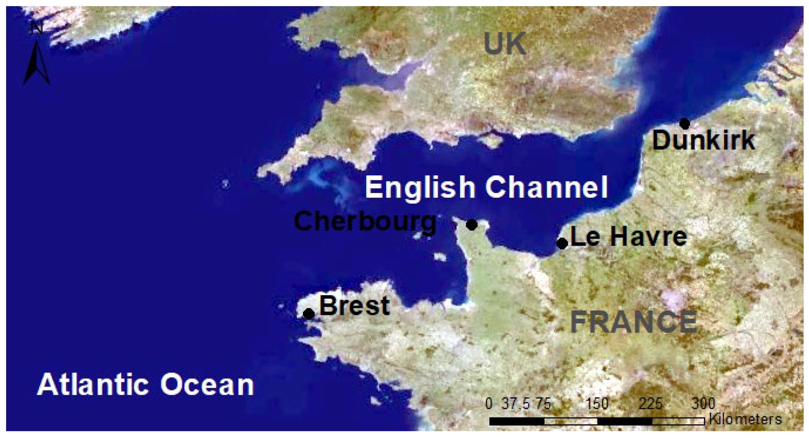
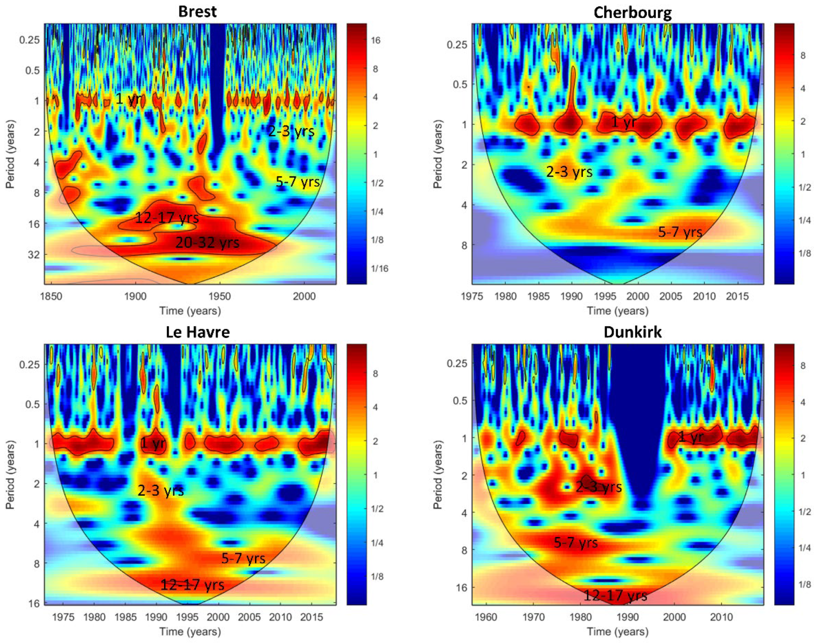
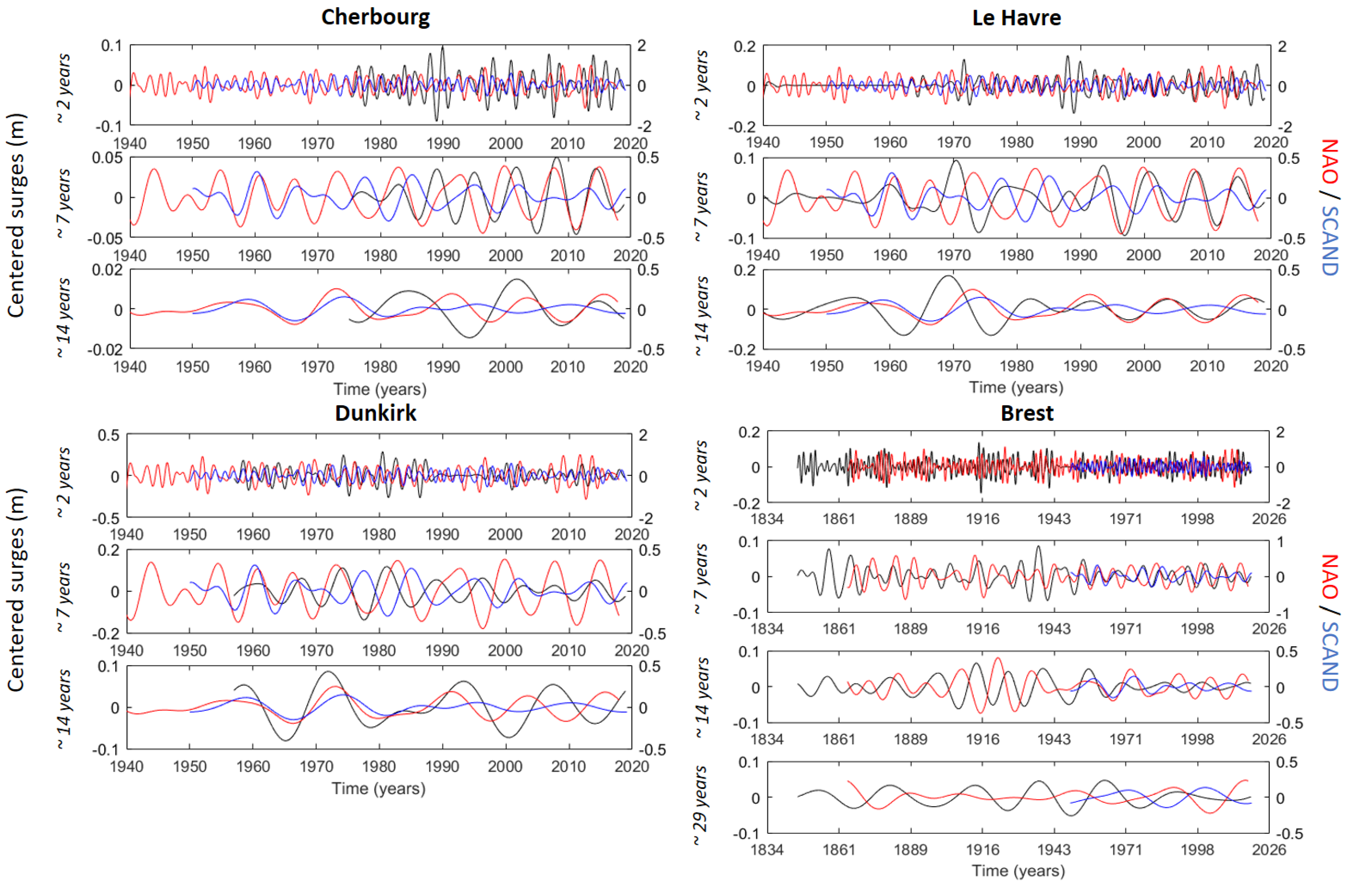
3.1.1. Extreme Surge Variability along the North French Coast (Brest to Dunkirk)

The wavelet spectra (Figure 5) displayed common timescales of variability: ~1 year, ~2–3 years, ~5–7 years, and ~12–17 years. The ~1-year variability can be related to the seasonality of monthly maxima surges with most of the higher maxima happening in winter every year. Sometimes, this variability showed an increased amplitude, such as 1990 at Brest, Cherbourg, Le Havre, when the winter monthly maxima were particularly high. When this happened for several years, we observed an increase in the amplitude of the ~2–3-year variability (e.g., for years around 1990). Indeed, between 1987 and 1991, there were numerous storm events of exceptional strength (e.g., the hurricane (1987), Daria (1990), Meteo France database (http://tempetes.meteofrance.fr/, accessed on 1 June 2019)). At Dunkirk, the ~2–3-year variability appeared to be particularly intense before the 1990s and then showed a decrease in amplitude after the 1990s. A similar phenomenon was found for the ~5–7-year variability.

Continuing at lower frequencies, all stations situated in the English Channel and Brest showed an increase in the ~5–7-year variability from around 1980 to the present day, whereas this increase appeared approximatively between 1965 and 1990 at Dunkirk. Dunkirk and Le Havre also displayed a ~12–17-year variability over the entire time series, while in Brest, this variability was statistically significant between 1890 and 1960 (Figure 5).

Most of the low frequencies (i.e., timescales higher than one year in this study) were not statistically significant, especially for time series starting after ~1960 (Cherbourg, Le Havre, Dunkirk). In contrast to these three stations, the monthly maxima at Brest showed a statistically significant ~12–17-year variability before 1950. This could indicate a decrease in variance for the ~12–17-year variability after 1950 for all stations. In parallel, the ~20–32 year variability in Brest was statistically significant, but this did not appear in the Cherbourg, Le Havre, and Dunkirk time series, because they are too short. The standard deviation and energy of wavelet details defined by the multiresolution analysis (MODWT) are presented in

Table 1. Fourier periods (Fperiod—years), standard deviation (Sd—m), and percentage of energy (Energy—%) of each wavelet detail (D) and the smooth (S) of monthly maxima surges. The total energy (Sum—%) of all wavelet details and the last smooth is also indicated.

Dunkirk	D1	D2	D3	D4	D5	D6	D7	D8	D9	S9	Sum
Fperiod	0.23	0.5	1	2	3.9	6.9	12.4	31	62	-	-
Sd	0.14	0.09	0.16	0.10	0.07	0.05	0.05	0.07	0.13	0.01	-
Energy	19.9	9.0	27.9	10.8	4.9	3.1	2.5	5.1	16.6	0.1	100
Le Havre	D1	D2	D3	D4	D5	D6	D7	D8	D9	S9	Sum
Fperiod	0.28	0.49	1	1.84	4.5	7.36	16.2	27	81	-	-
Sd	0.11	0.08	0.12	0.05	0.05	0.05	0.07	0.06	0.05	0.03	-
Energy	22.1	12.1	29.3	4.3	4.1	4.2	9.2	7.4	5.1	2.1	100
Cherbourg	D1	D2	D3	D4	D5	D6	D7	D8	D9	S9	Sum
Fperiod	0.2	0.46	1	2	4.9	6.29	14.67	22	44	-	-
Sd	0.09	0.07	0.11	0.04	0.03	0.03	0.01	0.01	0.01	0.00	-
Energy	30.5	17.2	40.2	5.9	2.9	2.4	0.32	0.43	0.28	0.0	100
Brest	D1	D2	D3	D4	D5	D6	D7	D8	D9	D10	D11	S11	Sum
Fperiod	0.23	0.38	1	1.88	3.84	7.86	14.42	28.83	57.67	86.5	173	-	-
Sd	0.09	0.07	0.09	0.05	0.03	0.03	0.03	0.03	0.01	0.01	0.01	0.00	-
Energy	30.9	18.4	28.4	8	4.3	3.2	3.0	2.4	0.8	0.5	0.1	0.0	100

. It is clear that, individually, low frequencies show lower variance (percentage of energy lower than 10%) than the annual variability (percentage of energy ranging from 25% to 40%), regardless of the sea-level station considered. Although low-frequency variabilities were generally not statistically significant and explained a small part of the total variability, they remained responsible for the increase in amplitude of the monthly maxima surges at some specific periods. Moreover, the spots of increased variability appeared over the same periods for different stations (e.g., for the ~5–7-year variability from around 1980 for stations in the English Channel and Brest). Therefore, these common patterns might have been generated by the same large-scale atmospheric drivers that we investigate in the next section.

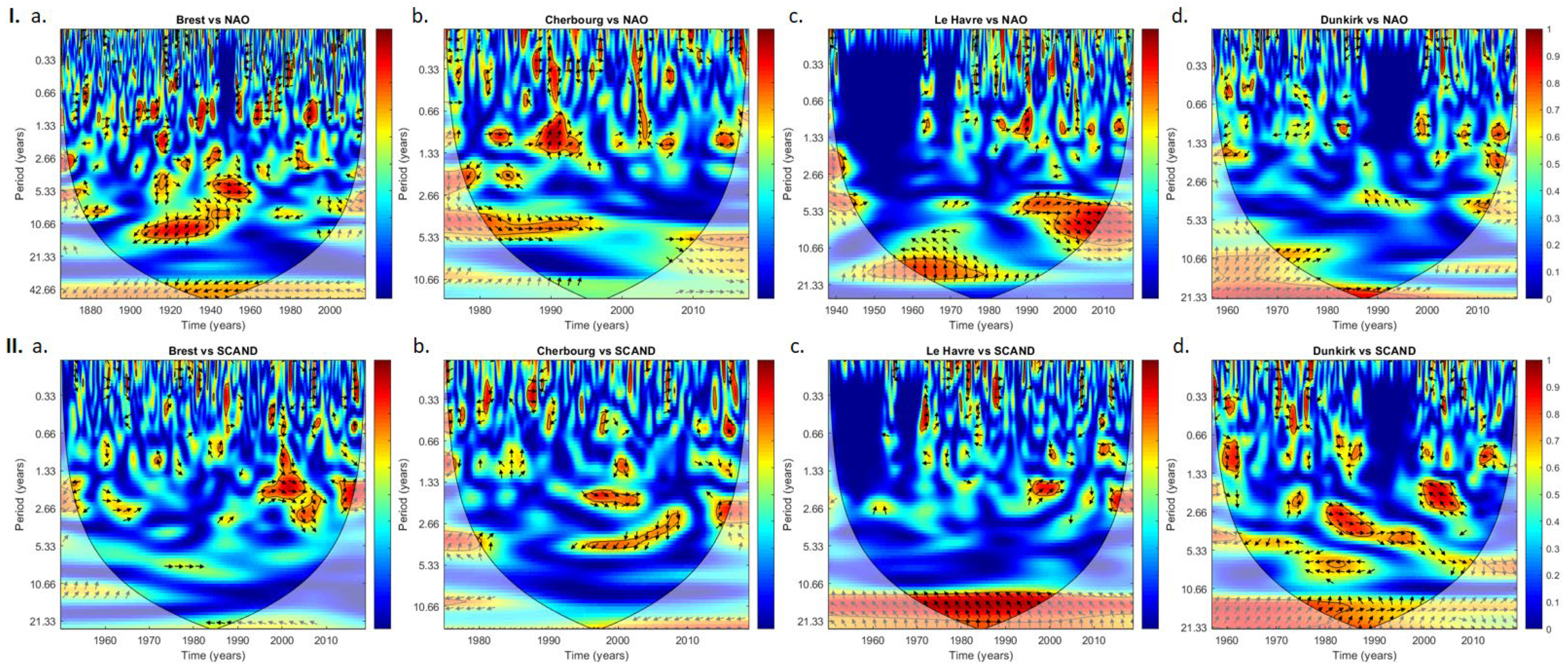
3.1.2. Influence of Large-Scale Atmospheric Circulation on Extreme Surges

Wavelet coherence and a MODWT analysis were conducted to identify large-scale atmospheric drivers responsible for the low-frequency variability in monthly maxima surges (Figure 6 and Figure 7). The standard deviation and wavelet detail energy of the climate indices defined with the MODWT are presented in

Table 2. Fourier periods (Fperiod—years), standard deviation (Sd—m), and percentage of energy (Energy—%) for each wavelet detail of monthly NAO and SCAND. The total energy (Sum—%) of all wavelet details and the last smooth is also indicated. Details highlighted in red are those introduced into GEV parameters in Section 3.2.2.

NAO	D1	D2	D3	D4	D5	D6	D7	D8	D9	D10	S10	Sum
Fperiod	0.17	0.50	1.00	2.39	3.56	7.65	17.00	30.6	76.5	153.0	-	-
Sd	1.140	0.879	0.670	0.453	0.335	0.281	0.168	0.102	0.112	0.084	0.033	-
Energy	43.7	25.9	15.1	6.9	3.8	2.6	0.9	0.3	0.4	0.2	0.0	100
SCAND	D1	D2	D3	D4	D5	D6	D7	D8	D9	S9	Sum
Fperiod	0.17	0.50	1.00	1.98	4.00	8.65	17.30	34.62	69.25	-	-
Sd	0.648	0.497	0.401	0.270	0.172	0.145	0.077	0.086	0.131	0.030	-
Energy	42.7	25.1	16.4	7.4	3.0	2.1	0.6	0.7	1.7	0.1	100

.

For Brest station, coherence between the monthly maxima and NAO was observed for the ~5–7-year and ~12–17-year variabilities (Figure 7(Ia)). The increase in the ~5–7-year variability at Brest from 1990 to the present could be related to the increase in variability of the NAO at this timescale (Figure 6). The coherence of the ~12–17-year variability between the monthly maxima and NAO was particularly significant over the 1900–1940 time period, which could be related to a rise in NAO variability that entails the same phenomenon in extreme surges (Figure 5, Figure 6 and Figure 7(Ia)). Unlike NAO, SCAND was shown to have less impact on Brest station (Figure 7(IIa)). Sporadic coherences were still noticeable at multi-annual timescales. Nevertheless, for the ~1.5–2.5-year variability, the coherence was higher than 0.8 in phase between 1995 and 2005. This element means that, during this period and for this timescale, monthly maxima surges are mainly impacted by SCAND. Beyond the ~1.5–2.5-year variability, all spots at lower frequencies presented rather low levels of coherence (still higher than 0.5) that were not statistically significant. Although the coherence of these spots was quite low, the two signals exhibited good phasing (e.g., around 1960–1965 for the ~2–3-year variability; 1970–1985 for the ~5–7-year variability). Furthermore, the significant spot at the ~20–32-year timescale for the monthly maxima surges did not seem to be related to the NAO, because there was no coherence at this timescale. No conclusion was reached for SCAND, because the timeseries is only available from 1950.

The monthly maxima for Cherbourg displayed roughly similar behavior to that of Brest: this station appeared to be more impacted by the NAO than SCAND. It also exhibited reasonably important coherence with the NAO for the ~5–7-year variability since the 2000s, and the two signals were found to be perfectly in phase (Figure 6 and Figure 7(Ib)). Nevertheless, the continuous wavelet transform of the Cherbourg monthly maxima displayed few differences in variance for the series before 2000 and after 2000: the spectral power remained significant over the whole period ~1985–2018 (Figure 5). Before 2000, the power was not much lower than in the 2000s. This could indicate that another factor could be part of the significant power of the ~5–7-year variability along with NAO. This other driver did not appear to be SCAND, because there were no common fluctuations with monthly maxima surges for this particular timescale from 1985 to the 2000s (Figure 6 and Figure 7(IIb)). As for Brest station, the Cherbourg monthly maxima exhibited sporadic coherence with SCAND, regardless of the considered timescale, although the coherence was higher.

The last station that exhibited strong coherence between its monthly maxima surges and NAO for the ~5–7-year and ~12–17-year variabilities was Le Havre (Figure 7(Ic)). As for Brest station, we noticed an increase in the ~5–7-year variability since the 1990s that might be related to the increase in the variability of NAO at this timescale since the 1970s (Figure 6). Moreover, the ~5–7-year variability of NAO and the monthly maxima surges has been almost in phase since the 1990s (Figure 6 and Figure 7(Ic)). Another coherence was seen for the ~12–17-year variability with NAO until 1980; however, no conclusions can be drawn from this, since many large gaps are present in the surge time series of Le Havre during this period. After 1995, monthly maxima surges were also found to be perfectly in phase with NAO at this timescale (Figure 6 and Figure 7(Ic)). Although the monthly maxima surges at Le Havre seem to be less impacted by SCAND than NAO, particularly for the ~5–7-year variability, large coherence with a significant phase shift was displayed by wavelet coherence for the ~12–17-year variability throughout the studied period (Figure 7(IIc)). Despite the phase shift between the two signals, we observed that variability and changes in the amplitude of monthly maxima surges and SCAND were quite similar: SCAND presented a decrease in amplitude from 1980 to the present (as did NAO) just like the monthly maxima surges (Figure 6). Therefore, the ~12–17-year variability of monthly maxima surges for Le Havre station could be impacted by NAO and SCAND.

Connections with these two regional large-scale atmospheric drivers appeared differently for Dunkirk station. Unlike other stations (Brest, Cherbourg and Le Havre), monthly maxima surges at Dunkirk appeared to be impacted by SCAND to a greater extent than NAO, particularly the ~5–7-year variability (Figure 7(Id,IId)). Although wavelet coherence with SCAND displayed coherence for most of the timescales, this was not constant over time. Indeed, between 1975 and 1985, the ~2–3-year variability of the monthly maxima surges expressed an important level of coherence that could be linked to an increase in SCAND variability that increased their variability (Figure 6 and Figure 7(IId)). We also identified a break in the coherence at around 1978, which might have contributed to a decrease in the monthly maxima surge variability (Figure 5, Figure 6 and Figure 7(IId)). As seen in the last section, the ~2–3-year variability of the monthly maxima surges at Dunkirk was characterized by a huge difference in variability before 1990 (stronger) and after 1990 (weaker) (Figure 5 and Figure 6), but this pattern did not seem to be related to SCAND (Figure 7(IId)). If that had been the case, we would have had a constant coherence for the ~2–3-year variability between SCAND and monthly maxima surges throughout the studied period.

At a lower frequency (~5–7 years), SCAND seemed to be linked to the increase in the Dunkirk monthly maxima surge variability between 1975 and 1990 due to its own increase in variability, and on the contrary, it was linked to the decrease in variability from 2000 to the present (Figure 6 and Figure 7(IId)). Finally, the ~12–17-year variability of the monthly maxima surges was highly coherent with SCAND (Figure 7(IId)). However, a decrease in coherence was noticeable in 1985, and SCAND did not express an increase in variability after 1990, which could have led to a noticeable increase in variability in the monthly maxima surges for Dunkirk after this date (Figure 5, Figure 6 and Figure 7(IId)). This means that, for the ~12–17-year variability, the monthly maxima surges at Dunkirk should have been dependent on another driver after 1990. This could be related to NAO, which exhibited an increase in variability after 1990 at this timescale and good coherence with the monthly maxima surges at Dunkirk (Figure 6 and Figure 7(Id)).

To summarize, monthly maxima surges at Dunkirk station showed different behavior to those at other stations. Indeed, monthly maxima surges at Dunkirk seemed to be more affected by SCAND (on the ~2–3-year, ~5–7-year, and ~12–17-year timescales) than other stations (particularly Brest and Cherbourg), which appeared to be more affected by NAO. In the English Channel, only Le Havre station on a ~12–17-year timescale seemed to be really impacted by SCAND. NAO appeared to primarily affect the low-frequency variabilities of Brest, Cherbourg, and Le Havre and, more specifically, the ~5–7 year variability from around 1985 where an increase in NAO variability generated a rise in the monthly maxima surge variability, while the ~5–7-year variability of the monthly maxima surges at Dunkirk seemed to be affected by SCAND. NAO was also shown to impact the ~12–17-year variability of the monthly maxima surges at Brest, Le Havre, and Dunkirk; while SCAND also impacted this variability at Le Havre and Dunkirk. Nevertheless, some amplitude modifications of some variabilities did not seem to be related to SCAND and NAO but were certainly due to another weather regime.

3.2. Analysis of Extreme Surges with Nonstationary GEV Models Using Climate Indices

3.2.1. Insertion of NAO and SCAND into the GEV Adjustment

Extreme surge events and surge variability are affected by large-scale atmospheric circulation. Thus, climate indices were introduced as covariates in the GEV parameters with the purpose of improving the GEV model quality. The results are expressed with the quality criterion described in Section 2.2.3. and are presented into the

Table 3. Improvement of the GEV model quality of monthly maxima surges through the introduction of NAO as a covariate to the location and location + scale parameters. Nonstationary models (SC and NAO) that express a lower AIC than that of the stationary model are better. Models that are highlighted in green were improved significantly (likelihood ratio test), and the p-value of the test is stated (threshold of 0.05). First, the introduction of the seasonal component was tested (likelihood ratio test between the stationary model and the nonstationary model with the introduction of the seasonal component). Second, the introduction of NAO as a covariate was tested (likelihood ratio test between the stationary model and the nonstationary model with NAO as a covariate). This study was not performed on the same temporal periods between stations due to climatic and sea-level data availability.

		Brest	Cherbourg	Le Havre	Dunkirk
Stationary model	AIC	−1424	−433	−84	152
Seasonal Component (SC)	AIC p-value	−1948 2 × 10−16	−650 2 × 10−16	−358 2 × 10−16	−140 2 × 10−16
NAO (μ)	AIC p-value	−1430 0.0061	−436 0.0277	−88 0.0139	152 0.1104
NAO (μ + ψ)	AIC p-value	−1429 0.0183	−443 0.0010	−104 7 × 10−6	146 0.0051

and

Table 4. Same as Table 3 but for the monthly SCAND.

		Brest	Cherbourg	Le Havre	Dunkirk
Stationary model	AIC	−653	−447	−78	152
Seasonal Component (SC)	AIC p-value	−933 2 × 10−16	−671 2 × 10−16	−355 2 × 10−16	−146 2 × 10−16
SCAND (μ)	AIC p-value	−667 6 × 10−5	−449 0.0569	−77 0.2385	152 0.1300
SCAND (μ + ψ)	AIC p-value	−667 0.0001	−447 0.1481	−75 0.4985	147 0.0102

.

First, the seasonal component clearly enhanced the GEV fitting of all stations because of the seasonal variability in the monthly maxima surges; this is well described by the annual timescale in the continuous wavelet spectra (Table 3 and Table 4, and Figure 5). The insertion of NAO improved the GEV models for Brest, Cherbourg, and Le Havre stations (Table 3). This is consistent with Section 3.1.2: these stations are mainly affected by NAO (Figure 7I). Dunkirk station fitting was also enhanced by NAO. Indeed, NAO was also found to be a driver of the low-frequency variability at Dunkirk station, particularly for the ~12–17-year variability and for lower-frequency timescales (Figure 7(Id)).

Simultaneously, the insertion of SCAND as a covariate allowed the GEV models to be improved for the Brest and Dunkirk stations (Table 4). For Dunkirk station, this is consistent with the wavelet coherence presented in Section 3.1.2., which shows that monthly maxima surges are highly dependent on the SCAND variability (Figure 7(IId)): the introduction of SCAND as a covariate in the GEV model for Dunkirk improved the quality of the fitting. On the contrary, the wavelet coherence between the monthly maxima surges at Brest and SCAND did not show such significant coherence for low frequencies (greater than ~1 year) (Figure 7(IIa)). Nevertheless, we noticed the existence of a few spots showing a coherence higher than 0.5 with signals perfectly in phase (e.g., around 1992–2010 for the ~1.5–2.5-year variability; 1960–1965 for the ~2–3-year variability; and 1970–1985 for the ~5–7-year variability). Consequently, the introduction of this climate index improved the GEV model because few parts of these extremes were still forced by the low-frequency variability of the SCAND. The phasing of the low frequencies of the two signals (monthly maxima surges and climate indices) seems to be an important factor in obtaining a better fitting than that produced with the stationary model. Hence, despite the higher coherence values for the ~12–17-year variability for Le Havre (than those of Brest), the signals were not in phase, which certainly did not allow for better fitting. Concerning Cherbourg, the model expressed a lower AIC when SCAND was introduced as a covariate in its model, which might be related to the high level of coherence between 1995 and 2005 for the ~2-year variability with signals almost in phase. The nonsignificance of this improvement could be explained by the small part of variability expressed by these extreme surges at this period and timescale, as shown on the continuous wavelet with low power (Figure 5).

It is also interesting for Dunkirk station to see that the enhancement of fittings was realized only when a climate index (SCAND or NAO) was introduced into the location and scale parameters (Table 3 and Table 4). Therefore, the sensitivity of extreme surges to the climate variables at Dunkirk is more important on the dispersion parameters. Overall, when the introduction of these climate covariates allowed the quality of models to improve, in most cases, the models were better when SCAND or NAO was introduced to the location and scale parameters (Cherbourg, Le Havre, and Dunkirk). However, for Brest station, the GEV fitting was better when NAO and SCAND were introduced only on the location parameter (Table 3 and Table 4).

3.2.2. Insertion of NAO and SCAND Spectral Components into the GEV Models

After assessing the effect of the NAO and SCAND “raw” indices (i.e., without decomposition) on the fitting quality, we aimed to assess whether the insertion of specific spectral components into GEV parameters could also allow the enhancement of the model quality (and under what conditions) and whether this improvement was better than the one obtained with the raw index.

The Brest GEV model was improved by the insertion of the ~2-year variability of NAO and SCAND (

Table 5. Same as for Table 3 and Table 4 but with NAO spectral components.

		Brest	Cherbourg	Le Havre	Dunkirk
Stationary model	AIC	−1424	−433	−84	152
Seasonal Component (SC)	AIC p-value	−1948 2 × 10−16	−650 2 × 10−16	−358 2 × 10−16	−140 2 × 10−16
~2.5 years (μ)	AIC p-value	−1428 0.0149	−432 0.4121	−84 0.1832	154 0.9715
~2.5 years (μ+ψ)	AIC p-value	−1426 0.0517	−431 0.4431	−86 0.0743	155 0.4538
~3.5 years (μ)	AIC p-value	−1422 0.9567	−432 0.3094	−83 0.5020	152 0.1877
~3.5 years (μ+ψ)	AIC p-value	−1422 0.3761	−430 0.5412	−81 0.7014	149 0.0269
~7.5 years (μ)	AIC p-value	−1423 0.3340	−432 0.3579	−88 0.0139	154 0.4365
~7.5 years (μ + ψ)	AIC p-value	−1422 0.4559	−432 0.2667	−93 0.0021	153 0.1949
~17 years (μ)	AIC p-value	−1424 0.1636	−431 0.5250	−83 0.4208	152 0.1526
~17 years (μ + ψ)	AIC p-value	−1424 0.2182	−430 0.6986	−85 0.1056	150 0.0546

and

Table 6. Same as for Table 3 and Table 4 but with SCAND spectral components.

		Brest	Cherbourg	Le Havre	Dunkirk
Stationary model	AIC	−653	−447	−78	152
Seasonal Component (SC)	AIC p-value	−933 2 × 10−16	−671 2 × 10−16	−355 2 × 10−16	−146 2 × 10−16
~2 years (μ)	AIC p-value	−657 0.0143	−446 0.4364	−76 0.8227	154 0.7850
~2 years (μ + ψ)	AIC p-value	−656 0.0380	−445 0.4839	−75 0.5169	153 0.2616
~4 years (μ)	AIC p-value	−652 0.3141	−445 0.9150	−77 0.2297	154 0.6138
~4 years (μ + ψ)	AIC p-value	−650 0.5879	−445 0.3381	−75 0.4333	150 0.0598
~8.5 years (μ)	AIC p-value	−652 0.4300	−446 0.4420	−76 0.5533	154 0.7038
~8.5 years (μ + ψ)	AIC p-value	−655 0.0582	−444 0.6963	−74 0.8286	156 0.9293
~17.5 years (μ)	AIC p-value	−652 0.2534	−447 0.2277	−80 0.0408	154 0.7318
~17.5 years (μ + ψ)	AIC p-value	−652 0.2203	−445 0.4090	−78 0.0934	154 0.3142

). Despite the noticeable coherence at lower frequencies with NAO, signals were generally out of phase when looking at the corresponding timescales on the wavelet coherence spectrum (Figure 7(Ia)). This probably did not allow the GEV model to be improved by the lower frequencies of NAO (Table 5). Concerning the ~2-year variability of SCAND, the improvement was certainly due to the high coherence (with signals in phase) between 1995 and 2005 (Table 6 and Figure 7(IIa)). Furthermore, monthly maxima surges and SCAND were in phase at the ~8.5-year timescale, but the coherence was quite low (~0.5). The phasing of signals certainly allowed the AIC criterion to be lower than the AIC of a stationary model, while the reasonably low coherence did not allow this improvement to be statistically significant. Moreover, the ~2-year variability of the monthly maxima surges at Brest contained a greater percentage of energy (8%) compared with the ~8-year variability (~3%), which could also explain why the enhancement by the latter was not statistically significant (Table 1).

The Cherbourg GEV model was not improved by the introduction of NAO or SCAND spectral components (Table 5 and Table 6). This was rather unexpected considering the high coherence between the low frequencies of Cherbourg monthly maxima surges and NAO, for instance (Figure 7(Ib)). Nevertheless, this could be explained by the fact that low frequencies at Cherbourg station only represent a small part of the total energy (~12%) (Table 1). Thus, most of the extreme surge variability at Cherbourg can be explained by local effects expressed at higher-frequency timescales, while regional climate effects seem to be less marked.

The Le Havre GEV model was improved significantly by only one component of each index: the ~7.5-year variability of NAO and the ~17.5-year variability of SCAND (Table 5 and Table 6). The NAO-related improvement is probably due to the high coherence between the monthly maxima surges and NAO for the ~7.5-year variability since 1995, while the signals presented good phasing (Figure 7(Ic)). The enhancement induced by the introduction of the ~17.5-year variability of SCAND could be related to the extremely high coherence (~1), even though signals were in quadrature (Figure 7(IIc)). This particular case is the only one in the present study that allowed better fitting while signals were not almost in phase.

Finally, the Dunkirk GEV model was never statistically significantly improved by the introduction of SCAND spectral components on the location and scale parameters (Table 6). This result was quite unexpected considering that the inclusion of the SCAND raw index improved the fitting and that a high coherence with SCAND was observed at some specific timescales (e.g., the ~4-year timescale). Nonetheless, the AIC still revealed better fitting when the SCAND ~4-year variability was introduced into the location and shape parameters of the GEV fitting. This SCAND variability was the only one to exhibit covariability in phase with that of the monthly maxima surges at Dunkirk. Simultaneously, the NAO ~3.5-year and ~17-year variabilities allowed for a better fitting quality (Table 5). Thus, as expressed in Section 3.2.1., the NAO ~17-year component is probably one of the two key components allowing for the enhancement of fittings in Dunkirk by NAO. The NAO ~3.5-year variability appeared to be the most significant component allowing for better fitting. When we look at the wavelet coherence between the monthly maxima surges at Dunkirk and NAO, a relatively high degree of coherence with signals almost in phase occurred from 2008 for this timescale (Figure 7(Id)). It is also interesting to highlight the better quality of models when these spectral components were introduced on the location and scale parameters as well as the NAO raw index (Table 3 and Table 5).

These results highlight the importance of phasing between low frequencies of SCAND or NAO and those of the monthly maxima surges for the improvement of GEV fitting. They also underline the fact that there is not a specific spectral component of a given climate index that allows for better enhancement of models. It is highly dependent on the considered station and the covariability of the low frequencies between monthly maxima surges and climate indices. Thus, spectral components of NAO that allow for better fitting than a stationary model are, respectively, the ~2.5-year variability for Brest, the ~7.5-year variability for Le Havre, and the ~3.5 year and ~17 year variabilities for Dunkirk. Simultaneously, spectral components of SCAND that allow for better fitting than a stationary model are, respectively, the ~2-year variability for Brest and the ~17.5-year variability for Le Havre.

Generally, the best fitting was achieved when the NAO spectral components were introduced into the location and scale parameters (Table 5). This was the case for Le Havre and Dunkirk stations. In contrast, for Le Havre, the best fitting with the ~17.5-year SCAND spectral component was obtained when it was introduced only in the location parameter (Table 6). For Brest station, this was the insertion of the SCAND or NAO spectral component only on the location parameter, which allowed the GEV fitting to be improved (Table 5 and Table 6). Except for the introduction of the SCAND ~17.5-year variability in the Le Havre GEV model, these results are identical to those obtained with raw climate indices.

4. Discussion

The impact of NAO on the sea-level variability has been analyzed in several studies. For Atlantic European coastlines, [39,40] described the proportionality between NAO values and the increase in winter storms, which affect extreme surges. For the Bristol Channel/Severn Estuary, [41] highlighted the influence of NAO on wind speed. According to their study, positive NAO phases induce higher wind speeds and, therefore, cause increases in the maximum extreme and mean sea levels. Moreover, several studies have addressed the physical mechanisms explaining the effects of continuous changes in NAO patterns on the sea-level variability [7,42].

The investigation of the low-frequency variability of sea levels has shown the existence of long-term oscillations that originate from large-scale, reginal climate variability and, thus, control the interannual extreme surges. The present analysis of monthly maxima surges across the North French coast exhibited the ~2–3-year and ~5–7-year variabilities. These variabilities were also investigated in several studies that explored sea-level variability and are commonly discussed in the literature, particularly for the Baltic sea [14,43,44]. These two typical variabilities were also identified in the total sea level and surges for Dunkirk, Le Havre, and Cherbourg in [3]. These oscillations were associated with large-scale atmospheric circulation and, in particular, with NAO [14]. We also distinguished a ~12–17-year variability in the monthly maxima surges at Brest that we attributed to NAO variability according to the wavelet coherence. This specific variability was also identified by [14] for the sea level at Brest, and they suggested that this may be related to the 13–15-year variability in SST exhibited by [45] and to the thermohaline circulation variability in the Atlantic Ocean [46,47,48]. Knowing the physical links between internal ocean variability and atmospheric circulation, it is expected that these two phenomena (thermohaline circulation and NAO) can be defined as two drivers of sea level/surge variability. For instance, [49] suggested that Gulfstream front interannual oscillations induce variability at the same timescale in the North Atlantic atmospheric circulation (i.e., in NAO). Thus, the ~12–17-year variability of the monthly maxima surges at Brest can be related to NAO and the thermohaline circulation variability.

In the present study, we focused on stations located on the northern French Coast, and two climate indices were chosen to represent two different weather patterns: NAO, representing zonal circulation, and SCAND, representing a blocking regime. Wavelet coherence and multiresolution analysis showed a higher influence of NAO on monthly maxima surges at Brest, Cherbourg, and Le Havre, while SCAND seemed to have a higher influence on the monthly maxima at Dunkirk. This is consistent with the study presented in [17], which showed a significant correlation between NAO and the 99th percentile of total sea level anomaly at Le Havre and Cherbourg. Nevertheless, their study did not show any significant correlations between NAO and the Brest time series.

These discrepancies in the correlations could be explained by the variable chosen to describe the extreme events (e.g., values above a threshold, monthly maxima, etc.), or by the climate indices used (e.g., winter or monthly NAO). In addition, previous studies demonstrated correlations between sea levels or surges and climate indices are not constant over time [14]. In the present work, wavelet coherence highlighted the dependence of correlation on the timescale and the time period. In this part of the study, it was demonstrated that variations in extreme surges (monthly maxima) are related to different atmospheric patterns (NAO and SCAND) according to the timescale and time period. On the other hand, these two indices did not explain the entire low-frequency variability of the monthly maxima surges, because there were periods where no coherence was expressed. Therefore, other weather patterns could have affected surges during these time periods (e.g., the Atlantic Ridge regime well represented by the EAP) or even the multidecadal oceanic variability. Nevertheless, in this study, each timescale was shown to have its best relationship with SCAND or NAO for a given time period. It should be highlighted that these two climate drivers act as regulators, controlling the extreme surge multi-timescale variability along the north French coast.

The introduction of the SCAND and NAO climate indices as covariates clearly improved GEV fitting in some previous studies [6,18,19]. In the present study, similar results were eventually reached, with a degree of model improvement found to depend rather significantly on the station considered but also on the nonstationarity of correlations over time. In [6], significant sensitivity of extreme sea levels to SCAND was found for the Brest and Dunkirk stations, while for Cherbourg, the sensitivity to SCAND was not significant, which was also the case in our study (Table 4). Indeed, the introduction of the SCAND as a covariate into the GEV parameters improved significantly Brest and Dunkirk models. In [6], results concerning NAO were similar to ours with a significant sensitivity found for Brest (Table 3). Le Havre station was not explored in their study; our analysis revealed an enhancement of the fitting when NAO was introduced as a covariate into the GEV model. This result is probably strongly related to the location of this station at the mouth of the Seine river, and its streamflow variability is known to be impacted by NAO [33]. This area is, therefore, highly impacted by NAO and the streamflow variability also impacts the sea level variability at Le Havre via surges [50]. These similar results to [6] enhance the idea that extreme surges induced by climate pattern are the main factor responsible for extreme sea level variability. Similar model enhancements to those shown in our study were found with NAO for Cherbourg and Dunkirk stations, and this can easily be explained by wavelet coherence.

Thus, we expect that the introduction of the spectral components of NAO and SCAND could also improve GEV fitting. This assumption was made, because these indices demonstrated great coherence with the corresponding monthly maxima surge spectral components. In most cases, the results showed that GEV fitting was improved when the coherence was higher than 0.5 with signals (monthly maxima surge spectral components and the corresponding of NAO or SCAND) roughly in phase at specific temporal periods. On the contrary, the model did not show any improvement if there was no coherence or when the signals were not approximatively in phase. This observation suggests that wavelet coherence is a powerful tool that may allow us to better understand the improvement of GEV models.

Sometimes, when we look at specific timescales on the wavelet coherence spectrum, we can clearly identify high coherence with signals in phase. Therefore, we can assume that this specific timescale of the considered climate index will allow significant improvement of the GEV model. Nevertheless, it is not always the case. A plausible interpretation of this phenomenon could be that the variety of components constituting the monthly maxima surges contributes to the established relationship between the corresponding spectral components of the two variables being hidden. Therefore, the relationship is no longer obvious.

Simultaneously, tests were carried out (not shown) in which a mathematical seasonal component and a spectral component of NAO and SCAND were combined in the nonstationary GEV model. It turned out that, for some specific components (such as the ~2-year component of SCAND in the GEV model), this association led to a decrease in model quality. Consequently, this highlights that the seasonal component introduced into the model can sometimes interfere with the results, masking the covariability with the spectral component of the given climate index.

The introduction of selected spectral components of either NAO or SCAND as covariates into GEV parameters did not allow for better improvement of the models, compared to that achieved with the raw climate index (higher AIC). Two plausible interpretations can be suggested to explain this result:

• The multi-year, low-frequency components of climate indices, even if retrieved in monthly maxima surges, never represented a very significant part of the total variance of the monthly maxima surge signals. Indeed, these components explained less than 50% of the explanatory percentage of energy for all stations. Multi-year to multi-decadal components explained, respectively, ~43% of total variance for Dunkirk, ~36% for Le Havre, ~22% for Brest, and only ~12% for Cherbourg. As a result, although correlation (as indicated by the wavelet coherence) seemed clear at such timescales, it would only allow for a small part of the extreme surges to be modelled. Thus, it could easily explain why the GEV models for Cherbourg station never improved with the introduction of the low-frequency spectral component of the NAO index, while the raw index allowed it.
• The nonstationarity of the large-scale climate relationships with local surge processes, as the wavelet coherence results showed that the large-scale/surge relationships were not constant over time for any timescale. This means that different low-frequency components would be involved in the relationships over time. As a result, considering each component separately as a covariate would only partially improve the GEV models.

Although the introduction of low-frequency components of climate indices did not improve the GEV models better than raw indices, it allowed us to highlight some interesting results. For instance, for Le Havre station, the introduction of NAO ~6–10-year variability induced a significant improvement in the GEV model. It was revealed that this NAO component is the main driver of extreme surges variability by influencing the 5–7-year surge variability. This NAO variability displayed significant coherence with the monthly maxima surges from approximatively 1990 onwards, which is also consistent with the results of [2], who showed that for a ~7-year oscillation timescale, the variability of monthly maximum surge amplitudes could be associated with a dipolar pattern of SLP fields over the North Atlantic Ocean, reminiscent of typical NAO-like western circulation. The exact same result was highlighted by [26] for both precipitation in northern France and Seine river streamflow. Since Le Havre station is located at the Seine mouth, the similar findings for Le Havre surges and the Seine river hydrological variability seem appropriate.

5. Conclusions

The aim of this study was (i) to identify the main timescales of variability for monthly maxima surges along the northern French coast and (ii) to examine their statistical links with two typical weather regimes: the zonal circulation (NAO) and blocking (SCAND) regimes. Continuous wavelet transform revealed common multi-year modes of variability in monthly maxima surges for the 4 stations studied: ~2–3 years, ~5–7 years, and ~12–17 years. The wavelet coherence results showed better correlations between low-frequencies of monthly maxima surges at Brest, Cherbourg, and Le Havre and NAO, while monthly maxima surges at Dunkirk seemed more covarying with SCAND. The coherence for each timescale was not constant over time, which demonstrated the nonstationary behaviour of the large-scale climate and extreme surge relationship. This finding explains the key role of climate patterns in extreme surge multi-timescale variability.

NAO and SCAND were introduced as covariates into parameters of GEV models to allow us to determine whether their introduction would improve the models; this was confirmed. Then, the characteristic timescales of these two climate indices were introduced into GEV models separately in order to identify the most forcing frequency on the GEV models and to assess whether this approach could improve the models even further. The results demonstrated that climate index spectral components with a coherence level of higher than 0.5 and good phasing with the corresponding spectral component of monthly maxima surges allowed for improved stationary GEV models. This highlights the usefulness of wavelet coherence to interpret these results. Nevertheless, compared with GEV models in which the raw index was introduced, only accounting for particular low-frequency components was less efficient overall.

Our results suggest that, as climate indices cannot explain all of the low-frequency variability in the monthly maxima surges, it would probably be more appropriate for prediction purposes to define an index from either the SLP or another large-scale field (e.g., 500 mb geopotential heights). Moreover, the integration of climate patterns into extreme models improves interannual forecasting and could be useful for General Circulation Model (GCM) simulations, which are designed to investigate physical mechanisms explaining teleconnections between the atmospheric circulation and sea-level variability.

References

1. Wong, P.P.; Losada, I.J.; Gattuso, J.-P.; Hinkel, J.; Khattabi, A.; McInnes, K.L.; Saito, Y.; Sallenger, A. Coastal Systems and Low-Lying Areas. In Climate Change 2014: Impacts, Adaptation, and Vulnerability. Part A: Global and Sectoral Aspects. Contribution of Working Group II to the Fifth Assessment Report of the Intergovernmental Panel on Climate Change; Field, C.B., Barros, V.R., Dokken, D.J., Mach, K.J., Mastrandrea, M.D., Bilir, T.E., Chatterjee, M., Ebi, K.L., Estrada, Y.O., Genova, R.C., et al., Eds.; Cambridge University Press: Cambridge, UK; New York, NY, USA, 2014; pp. 361–409. [Google Scholar]
2. Turki, I.; Massei, N.; Laignel, B. Linking Sea Level Dynamic and Exceptional Events to Large-Scale Atmospheric Circulation Variability: A Case of the Seine Bay, France. Oceanologia 2019, 61, 321–330. [Google Scholar] [CrossRef]
3. Turki, I.; Massei, N.; Laignel, B.; Shafiei, H. Effects of Global Climate Oscillations on Intermonthly to Interannual Variability of Sea Levels along the English Channel Coasts (NW France). Oceanologia 2020, 62, 226–242. [Google Scholar] [CrossRef]
4. Lowe, R.J.; Cuttler, M.V.W.; Hansen, J.E. Climatic Drivers of Extreme Sea Level Events Along the Coastline of Western Australia. Earth’s Future 2021, 9, e2020EF001620. [Google Scholar] [CrossRef]
5. Woodworth, P.L.; Melet, A.; Marcos, M.; Ray, R.D.; Wöppelmann, G.; Sasaki, Y.N.; Cirano, M.; Hibbert, A.; Huthnance, J.M.; Monserrat, S.; et al. Forcing Factors Affecting Sea Level Changes at the Coast. Surv. Geophys. 2019, 40, 1351–1397. [Google Scholar] [CrossRef] [Green Version]
6. Menéndez, M.; Woodworth, P.L. Changes in Extreme High Water Levels Based on a Quasi-Global Tide-Gauge Data Set. J. Geophys. Res. Ocean. 2010, 115, C10011. [Google Scholar] [CrossRef] [Green Version]
7. Marcos, M.; Calafat, F.M.; Berihuete, Á.; Dangendorf, S. Long-Term Variations in Global Sea Level Extremes. J. Geophys. Res. Ocean. 2015, 120, 8115–8134. [Google Scholar] [CrossRef] [Green Version]
8. Araújo, I. Sea Level Variability: Examples from the Atlantic Coast of Europe. Ph.D. Thesis, University of Southampton, Faculty of Engineering Science and Mathematics, School of Ocean and Earth Science, Southampton, UK, 2005. [Google Scholar]
9. Pirazzoli, P.A.; Costa, S.; Dornbusch, U.; Tomasin, A. Recent Evolution of Surge-Related Events and Assessment of Coastal Flooding Risk on the Eastern Coasts of the English Channel. Ocean Dynam. 2006, 56, 498–512. [Google Scholar] [CrossRef]
10. Haigh, I.; Nicholls, R.; Wells, N. Assessing Changes in Extreme Sea Levels: Application to the English Channel, 1900–2006. Cont. Shelf Res. 2010, 30, 1042–1055. [Google Scholar] [CrossRef]
11. Wahl, T.; Haigh, I.D.; Woodworth, P.L.; Albrecht, F.; Dillingh, D.; Jensen, J.; Nicholls, R.J.; Weisse, R.; Wöppelmann, G. Observed Mean Sea Level Changes around the North Sea Coastline from 1800 to Present. Earth-Sci. Rev. 2013, 124, 51–67. [Google Scholar] [CrossRef] [Green Version]
12. Mölter, T.; Schindler, D.; Albrecht, A.T.; Kohnle, U. Review on the Projections of Future Storminess over the North Atlantic European Region. Atmosphere 2016, 7, 60. [Google Scholar] [CrossRef] [Green Version]
13. Wakelin, S.L.; Woodworth, P.L.; Flather, R.A.; Williams, J.A. Sea-Level Dependence on the NAO over the NW European Continental Shelf. Geophys. Res. Lett. 2003, 30, 1403. [Google Scholar] [CrossRef]
14. Jevrejeva, S.; Moore, J.C.; Woodworth, P.L.; Grinsted, A. Influence of Large-Scale Atmospheric Circulation on European Sea Level: Results Based on the Wavelet Transform Method. Tellus A 2005, 57, 183–193. [Google Scholar] [CrossRef]
15. Ezer, T.; Haigh, I.D.; Woodworth, P.L. Nonlinear Sea-Level Trends and Long-Term Variability on Western European Coasts. J. Coast. Res. 2015, 32, 744–755. [Google Scholar] [CrossRef]
16. Woodworth, P.L.; Flather, R.A.; Williams, J.A.; Wakelin, S.L.; Jevrejeva, S. The Dependence of UK Extreme Sea Levels and Storm Surges on the North Atlantic Oscillation. Cont. Shelf Res. 2007, 27, 935–946. [Google Scholar] [CrossRef]
17. Marcos, M.; Woodworth, P.L. Spatiotemporal Changes in Extreme Sea Levels along the Coasts of the North Atlantic and the Gulf of Mexico. J. Geophys. Res. Ocean. 2017, 122, 7031–7048. [Google Scholar] [CrossRef] [Green Version]
18. Méndez, F.J.; Menéndez, M.; Luceño, A.; Losada, I.J. Analyzing Monthly Extreme Sea Levels with a Time-Dependent GEV Model. J. Atmos. Ocean Technol. 2007, 24, 894–911. [Google Scholar] [CrossRef]
19. Masina, M.; Lamberti, A. A Nonstationary Analysis for the Northern Adriatic Extreme Sea Levels. J. Geophys. Res. Ocean. 2013, 118, 3999–4016. [Google Scholar] [CrossRef]
20. Hurrell, J.W.; Van Loon, H. Decadal Variations in Climate Associated with the North Atlantic Oscillation. Clim. Change 1997, 36, 301–326. [Google Scholar] [CrossRef]
21. Cassou, C.; Terray, L.; Hurrell, J.W.; Deser, C. North Atlantic Winter Climate Regimes: Spatial Asymmetry, Stationarity with Time, and Oceanic Forcing. J. Clim. 2004, 17, 1055–1068. [Google Scholar] [CrossRef]
22. Comas-Bru, L.; McDermott, F. Impacts of the EA and SCA Patterns on the European Twentieth Century NAO–Winter Climate Relationship. Q. J. Roy. Meteor. Soc. 2014, 140, 354–363. [Google Scholar] [CrossRef]
23. Hurrell, J.W. Decadal Trends in the North Atlantic Oscillation: Regional Temperatures and Precipitation. Science 1995, 269, 676–679. [Google Scholar] [CrossRef] [PubMed] [Green Version]
24. Barnston, A.G.; Livezey, R. Classification, Seasonality and Persistence of Low-Frequency Atmospheric Circulation Patterns. Mon. Weather. Rev. 1987, 115, 1083–1126. [Google Scholar] [CrossRef]
25. Hurrell, J.W.; Deser, C. North Atlantic Climate Variability: The Role of the North Atlantic Oscillation. J. Mar. Syst. 2009, 78, 28–41. [Google Scholar] [CrossRef]
26. Massei, N.; Dieppois, B.; Hannah, D.M.; Lavers, D.A.; Fossa, M.; Laignel, B.; Debret, M. Multi-Time-Scale Hydroclimate Dynamics of a Regional Watershed and Links to Large-Scale Atmospheric Circulation: Application to the Seine River Catchment, France. J. Hydrol. 2017, 546, 262–275. [Google Scholar] [CrossRef] [Green Version]
27. Cornish, C.R.; Bretherton, C.S.; Percival, D.B. Maximal Overlap Wavelet Statistical Analysis With Application to Atmospheric Turbulence. Bound. Layer Meteorol 2006, 119, 339–374. [Google Scholar] [CrossRef]
28. Bortot, P.; Tawn, J.A. Joint Probability Methods for Extreme Still Water Levels and Waves; Lancaster University: Lancaster, UK, 1997. [Google Scholar]
29. Kergadallan, X. Estimation Des Niveaux Marins Extrêmes Avec et sans l’action Des Vagues Le Long Du Littoral Métropolitain. Ph.D. Thesis, Université Paris-Est, Champs-sur-Marne, France, 2015. [Google Scholar]
30. Torrence, C.; Compo, G.P. A Practical Guide to Wavelet Analysis. B. Am. Meteorol. Soc. 1998, 79, 61–78. [Google Scholar] [CrossRef] [Green Version]
31. Labat, D. Recent Advances in Wavelet Analyses: Part 1. A Review of Concepts. J. Hydrol. 2005, 314, 275–288. [Google Scholar] [CrossRef]
32. Massei, N.; Durand, A.; Deloffre, J.; Dupont, J.P.; Valdes, D.; Laignel, B. Investigating Possible Links between the North Atlantic Oscillation and Rainfall Variability in Northwestern France over the Past 35 Years. J. Geophys. Res. Atmos. 2007, 112, D09121. [Google Scholar] [CrossRef] [Green Version]
33. Massei, N.; Laignel, B.; Deloffre, J.; Mesquita, J.; Motelay, A.; Lafite, R.; Durand, A. Long-Term Hydrological Changes of the Seine River Flow (France) and Their Relation to the North Atlantic Oscillation over the Period 1950–2008. Int. J. Climatol. 2010, 30, 2146–2154. [Google Scholar] [CrossRef]
34. Grinsted, A.; Moore, J.C.; Jevrejeva, S. Application of the Cross Wavelet Transform and Wavelet Coherence to Geophysical Time Series. Nonlinear Proc. Geoph. 2004, 11, 561–566. [Google Scholar] [CrossRef]
35. Coles, S. An Introduction to Statistical Modeling of Extreme Values; Springer Series in Statistics; Springer: London, UK, 2001; ISBN 978-1-84996-874-4. [Google Scholar]
36. Coles, S.G.; Walshaw, D. Directional Modelling of Extreme Wind Speeds. J. Roy. Stat. Soc. C-App. 1994, 43, 139–157. [Google Scholar] [CrossRef]
37. Katz, R.W.; Parlange, M.B.; Naveau, P. Statistics of Extremes in Hydrology. Adv. Water Resour. 2002, 25, 1287–1304. [Google Scholar] [CrossRef] [Green Version]
38. Akaike, H. A New Look at the Statistical Model Identification. IEEE Trans. Autom. Control. 1974, 19, 716–723. [Google Scholar] [CrossRef]
39. Hulme, M.; Jenkins, G.J.; Lu, X.; Turnpenny, J.R.; Mitchell, T.D.; Jones, R.G.; Lowe, J.; Murphy, J.M.; Hassell, D.; Boorman, P.; et al. Climate Change Scenarios for the United Kingdom: The UKCIP02 Scientific Report; Tyndall Centre for Climate Change Research, School of Environmental Sciences, University of East Anglia: Norwich, UK, 2002; p. 120. [Google Scholar]
40. Lozano, I.; Devoy, R.J.N.; May, W.; Andersen, U. Storminess and Vulnerability along the Atlantic Coastlines of Europe: Analysis of Storm Records and of a Greenhouse Gases Induced Climate Scenario. Mar. Geol. 2004, 210, 205–225. [Google Scholar] [CrossRef]
41. Phillips, M.R.; Rees, E.F.; Thomas, T. Winds, Sea Levels and North Atlantic Oscillation (NAO) Influences: An Evaluation. Glob. Planet. Chang. 2013, 100, 145–152. [Google Scholar] [CrossRef]
42. Tsimplis, M.N.; Josey, S.A. Forcing of the Mediterranean Sea by Atmospheric Oscillations over the North Atlantic. Geophys. Res. Lett. 2001, 28, 803–806. [Google Scholar] [CrossRef] [Green Version]
43. Yan, Z.; Tsimplis, M.N.; Woolf, D. Analysis of the Relationship between the North Atlantic Oscillation and Sea-Level Changes in Northwest Europe. Int. J. Climatol. 2004, 24, 743–758. [Google Scholar] [CrossRef]
44. Medvedev, I.; Kulikov, E. Low-Frequency Baltic Sea Level Spectrum. Front. Earth Sci. 2019, 7, 284. [Google Scholar] [CrossRef]
45. Moron, V.; Vautard, R.; Ghil, M. Trends, Interdecadal and Interannual Oscillations in Global Sea-Surface Temperatures. Clim. Dyn. 1998, 14, 545–569. [Google Scholar] [CrossRef]
46. Deser, C.; Blackmon, M.L. Surface Climate Variations over the North Atlantic Ocean during Winter: 1900–1989. J. Clim. 1993, 6, 1743–1753. [Google Scholar] [CrossRef]
47. Rajagopalan, B.; Kushnir, Y.; Tourre, Y.M. Observed Decadal Midlatitude and Tropical Atlantic Climate Variability. Geophys. Res. Lett. 1998, 25, 3967–3970. [Google Scholar] [CrossRef] [Green Version]
48. Rodwell, M.J.; Rowell, D.P.; Folland, C.K. Oceanic Forcing of the Wintertime North Atlantic Oscillation and European Climate. Nature 1999, 398, 320–323. [Google Scholar] [CrossRef]
49. Feliks, Y.; Ghil, M.; Robertson, A.W. The Atmospheric Circulation over the North Atlantic as Induced by the SST Field. J. Clim. 2011, 24, 522–542. [Google Scholar] [CrossRef] [Green Version]
50. Turki, I.; Laignel, B.; Chevalier, L.; Costa, S.; Massei, N. On the Investigation of the Sea-Level Variability in Coastal Zones Using SWOT Satellite Mission: Example of the Eastern English Channel (Western France). IEEE J. Sel. Top. Appl. 2015, 8, 1564–1569. [Google Scholar] [CrossRef]
Figure 1. Location of sea level stations.
Atmosphere 13 00850 g001
Figure 2. Year-by-year availability of sea-level data from Brest, Le Havre, Cherbourg, and Dunkirk.
Atmosphere 13 00850 g002
Figure 3. Monthly maxima surges at Brest, Cherbourg, Le Havre, and Dunkirk.
Atmosphere 13 00850 g003
Figure 4. Boxplots of monthly maxima surges at Brest, Cherbourg, Le Havre, and Dunkirk. The lower parts of the boxes represent the 1st quartiles, the red lines represent the medians, and the upper parts represent the 3rd quartiles. The upper part and lower part of the dashed lines are, respectively, the maximum and minimum values for each month considered. The red marks are the outliers, i.e., values that are more than 1.5 times the interquartile range. Please note that the analysis using boxplots started in different years for the different stations (1846 for Brest, 1975 for Cherbourg, 1972 for Le Havre, 1957 for Dunkirk) but ended in 2018 for all stations. Note also that outliers were not omitted from the time series and computations in this article, since these values are not measurement errors but real extreme levels.
Atmosphere 13 00850 g004
Figure 5. Continuous wavelet spectra applied to monthly maxima surges at Brest, Cherbourg, Le Havre, and Dunkirk. The cone of influence is represented by continuous lines, and the area outside of this cone must not be interpreted because of the zeros introduced into the calculation of the spectrum. Spots surrounded by a continuous line are statistically significant (Monte-Carlo test). Please note that the Y axes are not at the same scale for all stations.
Atmosphere 13 00850 g005
Figure 6. Reconstruction of multi-year modes of variability of monthly maxima surges (black) at Cherbourg, Le Havre, Dunkirk, and Brest, and of SCAND (blue) and NAO (red) using MODWT.
Atmosphere 13 00850 g006
Figure 7. Wavelet coherence between (I) NAO and the monthly maxima at (a) Brest, (b) Cherbourg, (c) Le Havre, and (d) Dunkirk and (II) SCAND and the monthly maxima at (a) Brest, (b) Cherbourg, (c) Le Havre, and (d) Dunkirk. The arrows represent the phase between two signals: if the arrow points to the left, the signals are in antiphase; if the arrow points to the right, the signals are in phase; and if the arrow points at 90°, the signals are in quadrature. Surrounding spots are statistically significant (Monte–Carlo test).
Atmosphere 13 00850 g007