1. Introduction
The main component of haze is fine particulate matter (PM2.5), an organic compound of toxic substances such as heavy metals and carcinogens. It is the most harmful air pollution to the human body because it can directly enter the lungs [
1,
2,
3]. In recent years, more and more people have paid close attention to its environmental damage and influence on the human body in large urban areas [
4,
5,
6].
With the increased attention on haze, the harm it does to the human body is gradually being revealed. Therefore, the research on haze becomes deeper and more diverse [
7,
8,
9,
10,
11]. Predominant questions involve the causes of haze, pollution composition, time distribution, regional distribution, and management programs. The research methods also span multiple disciplines such as chemical analysis, biological testing, economic development, and haze data mining.
Because of the improved human aerospace technology and remote sensing satellite technology in recent years, the cost of remote sensing satellite imagery has been reduced. It is more macroscopic than the traditional ground station monitoring data. The satellite images provide the information of the temporal and spatial changes of haze comprehensively and quickly [
12,
13,
14,
15,
16,
17,
18]; therefore, researchers utilize remote sensing images in the monitoring and analysis of haze. Researchers often use remote sensing satellite images for the inversion of Aerosol Optical Depth (AOD) and further analyze meteorological features based on the correlation between aerosol depth and atmospheric pollutant concentrations. McGowan et al. [
19] proposed a PM10 dust concentration of a 500 m vertical profile measured during a regional dust event in western Queensland, Australia, based on MODIS Terra satellite data and a spatiotemporal analysis. Guo et al. [
20] used a correlation analysis between the PM2.5 concentration ground haze monitoring stations in China during 2007 and 2008 and the AOD obtained from the satellite remote sensing image. They also discussed the feasibility of satellite remote sensing technology for estimating the haze concentration on the ground. Nordio et al. [
21] used MODIS data to study the correlation between aerosol and PM10 concentration in Lombardy, Italy, and successfully used aerosol data to predict the haze concentration. Seo et al. [
22] compared the aerosol depth based on ground monitoring stations and MODIS satellite images to PM10 concentrations in Seoul, Korea. It was concluded that MODIS images are more relevant than ground monitoring stations, especially in winter.
Another emerging approach to haze research is machine learning. Machine learning methods, especially the rapid development of neural networks, have shown researchers great potential to fit complex functions. Therefore, some studies have used haze detection data to train neural networks to predict haze concentrations. For example, Pérez et al. [
23] used the neural network structure to predict and analyze the average concentration of haze in the San Diego area in the next few hours. Grivas et al. [
24] optimized the structure and parameters of the neural network based on the previous Pérez study to predict the concentration of PM10. With the continuous optimization of the network, many scholars have used neural networks to predict and analyze the haze in time series [
25,
26,
27,
28].
Comparing the two haze analysis methods, estimating the concentration of haze pollutants, such as PM2.5 and PM10, using the inversion of AOD on remote sensing satellite images has a broader research background and relative higher precision. However, the data preprocessing for obtaining AOD from satellite images is very complicated and often requires steps such as radiation correction, geometric correction, and processing angle data for satellite images. By contrast, neural networks have powerful feature capture capabilities and flexible adjustment capabilities using these learned features. These characteristics allow neural networks to use simplified data processing compared with traditional inversion methods. Moreover, the neural network excels in complex function fitting, making it easy to fit uncertain function expressions or expressions with complex parameters. In the study of haze, PM2.5 concentration prediction is a complex function fitting problem, since the concentration of other major pollutants such as PM2.5 depends on many complicated meteorological and human factors.
This paper aims to simplify complex data processing in traditional AOD inversion methods by using the feature capture ability and complex function fitting ability of neural networks by training a haze-level classification network. We directly use remote sensing satellite images as input and use convolutional neural networks as training models to classify the level of haze concentration. This paper compares the results from two methods, one using a traditional AOD inversion method, and the other the proposed neural networks inversion method. Experiments show that the proposed network can reduce the manual inversion work, and also achieves good results in fitting the non-linear relationship between the data and the haze concentration level.
2. Research Area and Dataset
2.1. Research Area
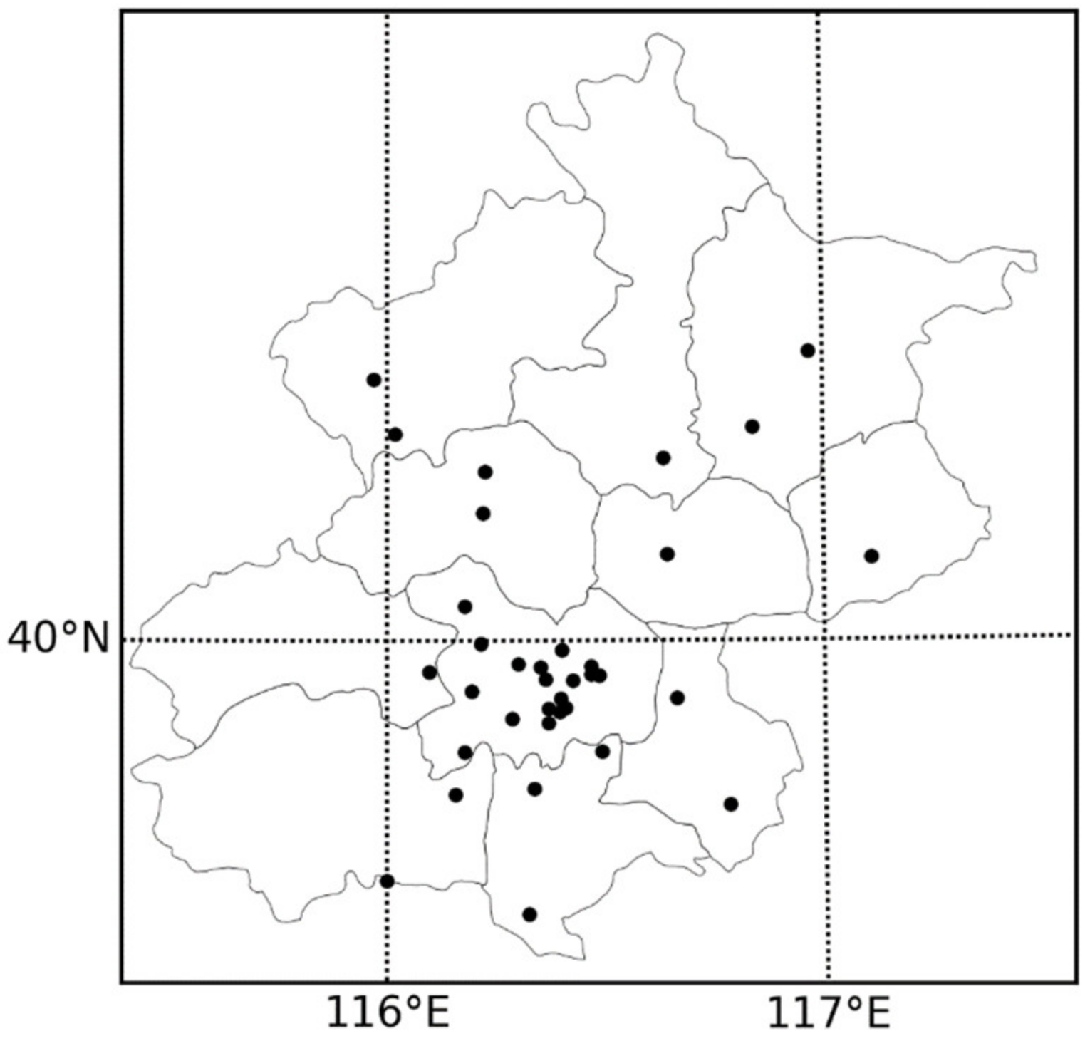
The air pollutant monitoring stations in the Beijing area mainly detect the concentration of various air pollutant gases (such as carbon monoxide, sulfur dioxide, and ozone) and PM1 and PM2.5. These monitoring stations are distributed in various districts of Beijing, as shown in
Figure 1. The data and monitoring records collected by the monitoring points will be published in real-time for easy access and research.
There are also some objective reasons for selecting the Beijing area for study. The Beijing area is one of the more effective observation points of NASA’s meteorological satellites, and it is also the network point of the ground aerosol automatic observation network (AREONET). Therefore, different data can be used for comparison. Moreover, Beijing is the capital of China, with a relatively high population density and frequent haze. Therefore, the significance and feasibility of the research are high.
2.2. Dataset
Satellite remote sensing data has solid spatial coverage. In remote sensing science, researchers invert images to obtain AOD and haze concentrations.
This paper hopes to simplify the data processing and replace the traditional AOD inversion method using the fitting ability of convolutional neural networks, and construct an end-to-end haze level prediction network. Considering the experimental needs, we collect several highly relevant experimental data:
- (1)
MOD02-1 km data for the Beijing area in 2013 and 2014. The MOD02-1 km is a satellite remote sensing image product of MODIS. The latitude and longitude are calibrated based on the original data. Subsequently, we will preprocess it and use the preprocessed data as training and testing data for the traditional inversion method of AOD and the haze level prediction network.
- (2)
Real-time haze concentration data covering the entire Beijing area in 2013. We will preprocess the dataset to obtain the haze level and use this to mark the satellite imagery of the 2013 Beijing area to build a complete training set.
- (3)
Real-time haze concentration data covering the entire Beijing area in 2014. The data include real-time PM2.5 concentrations and PM10 concentrations per hour for each day in 2014, and Air Quality Index (AQI) information. The data come from 36 automatic monitoring stations for atmospheric pollutants covering the entire main area of Beijing. The data will verify the correlation between haze concentration and AOD.
- (4)
AREONET ground monitoring aerosol data are used to verify the accuracy of aerosol inversion. This observatory will also provide three levels of data: Level 1.0 (unscreened), Level 1.5 (cloud-screened and quality controlled), and Level 2.0 (quality-assured). Among them, the observation accuracy of the AOD of L2 data is the highest.
- (5)
Remote sensing image products from AQUA and TERRA satellites equipped with MODIS. The MODIS product models are: MOD02-1 km (MYD-021 km) and MOD04-3 k (MYD04-3 k), secondary satellite products, and processed aerosol products. MOD02-1 km belongs to the L1b product, the original data after the latitude and longitude calibration, while MOD04-3 km is the processed second-level product containing multiple aerosol products.
3. Comparison with Traditional Method
In order to determine the type of data that can provide information regarding the haze concentration and the type of input data of the convolutional neural network, it is necessary to study the data used in the traditional inversion method. Then, from the data processing process used in the traditional method, the data type and processing method required by the convolutional neural network are analyzed and obtained. This section presents the traditional method selected to set up the convolutional neural network in order to obtain the required information. The method will also be used to examine the performance of the proposed neural network method.
The data processing process in the traditional method is as follows:
- (1)
Radiation correction: We used ENVI5.0 to read data from MOD02-1 km, and the software automatically radiated and corrected the data.
- (2)
Geometric correction: We used the MODIS data processing tool, Georeference MODIS in the ENVI software, to geometrically correct the data of the emissivity channel. In the calibration, we selected the Beijing coordinate system in the World Geodetic System 1984 (WGS-84) standard to geometrically correct the emissivity file and establish Ground Control Points (GCPs) as the standard for other channels to maintain consistent geometric correction results. We used GCPs generated by the emissivity to correct the reflectance file. After reading the GCPs, the triangulation correction method and the bilinear resampling method were selected so that the correction result of the reflectance can match the emissivity.
- (3)
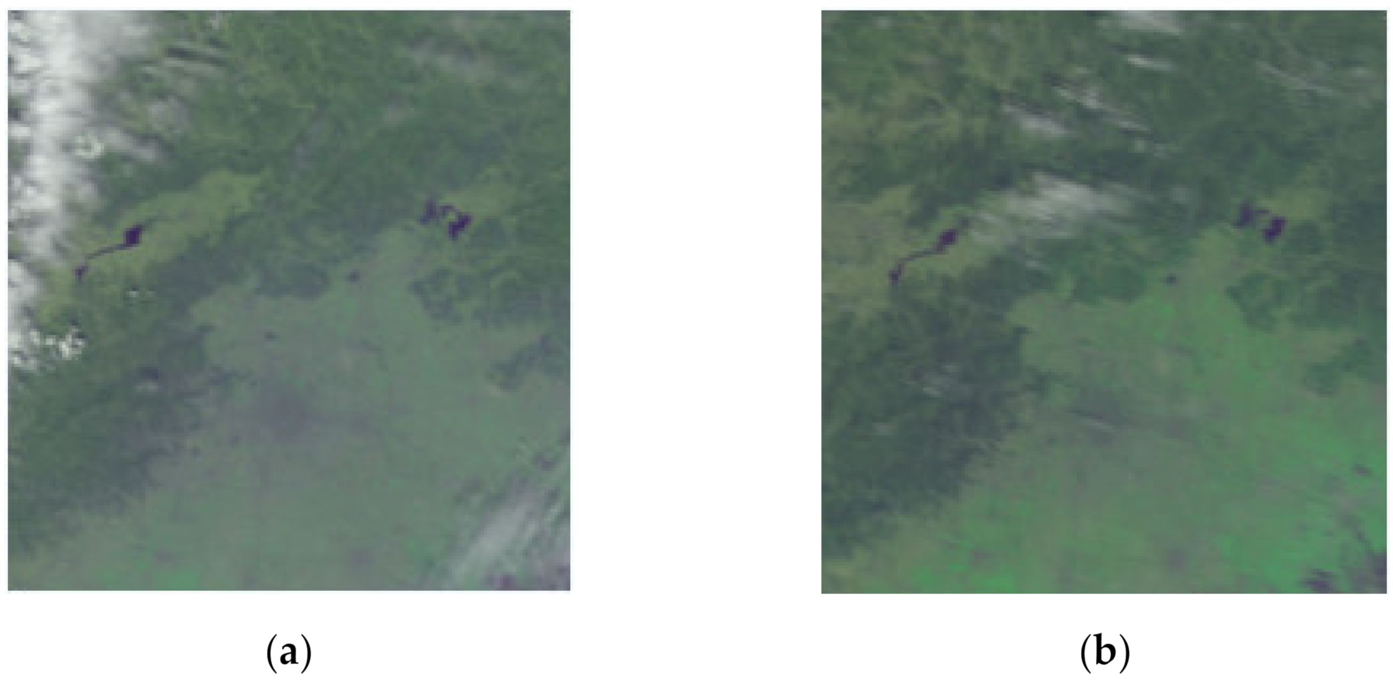
Interest area extraction and synthesis: We selected the administrative regional geographic graphic document (shapefile) in the Global Administrator Areas Database (GADM). According to the administrative area of Beijing: 39.4 N~41.1 N; 115.4~117.4 E, we tailored the emissivity and reflectivity file, which kept the consistency of the administrative scope and the size of the processed data. After the region of interest was synthesized, the emissivity channel files were placed at the top, and the reflectivity channel files were placed at the bottom. The result of the image processing is shown in
Figure 2.
- (4)
The processing of angle data: First, we used the ground control point file to correct the angle dataset geometrically and used the shape-file cutting angle data of the Beijing area, and then synthesized the angle data according to the order of the solar zenith angle, the solar azimuth angle, the satellite zenith angle, and the satellite azimuth angle. Finally, the time sequence stored the processed data for subsequent inversion processing.
- (5)
AOD inversion: The inversion method was the lookup table method (LUT): the lookup table file is a general-purpose file. Its content is a table of the relationship between radiation reflection, emissivity, angle data, and AOD. This paper used the aerosol inversion tool in ENVI to read the data results processed in steps (3) and (4). Then, it combined the relationship between the corresponding emissivity, reflectivity, angle, and AOD in the lookup table file to perform the aerosol inversion.
Through the operation of the above five parts, the inversion of the AOD was realized.
We can learn from previous researchers that there is a functional mapping between the optical depth of aerosol and the sun’s radiation. Holben et al. [
29] proposed a radiation transfer formula that combines AOD with radiation. The relationship between them is described as Equation (1).
in the above formula denotes a comprehensive signal of all reflected signals received by satellite, where denotes AOD. and denote the solar zenith angle and satellite zenith angle when the satellite passes through the region of interest, respectively. denotes the corresponding sun azimuth angle and satellite azimuth. denotes the reflected solar radiation by the atmosphere. denotes the solar radiation that is not reflected and injected into the atmosphere, and denotes the satellite emission signal that passes through the atmosphere. is the reflectivity of the ground to solar radiation. denotes the reflectivity of the atmosphere to the sun’s radiation.
4. CNN Haze Classification Method
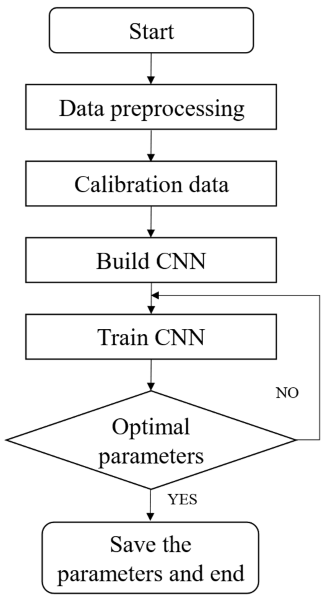
The convolutional neural network used in this research adopts an end-to-end idea. Therefore, the final training process is to fit this mapping relationship using a haze satellite remote sensing image as input, and the haze concentration level as output. The specific algorithm flow is shown in
Figure 3.
4.1. CNN Data Processing
When the traditional method retrieves the AOD and haze concentrations from remote sensing images, the information of these angles needs to be extracted, cut, and synthesized, and this process is relatively cumbersome. After evaluating the zenith and azimuth angles, we decided not to consider their changes since these angles are relatively fixed when the satellite passes through the same area in the same season. Therefore, when preprocessing the remote sensing data, the CNN method only needs to extract, cut, and synthesize the reflectivity and emissivity. After the data are processed as above, they are stored chronologically by season. Then, the convolution neural network is used to fit their non-linear relationship, and finally, the haze level is classified through the classification layer.
According to the channel information, the channels for monitoring the edge and characteristics of the land and cloud are 1–7 channels. The wavelength and spatial resolution of each channel are shown in
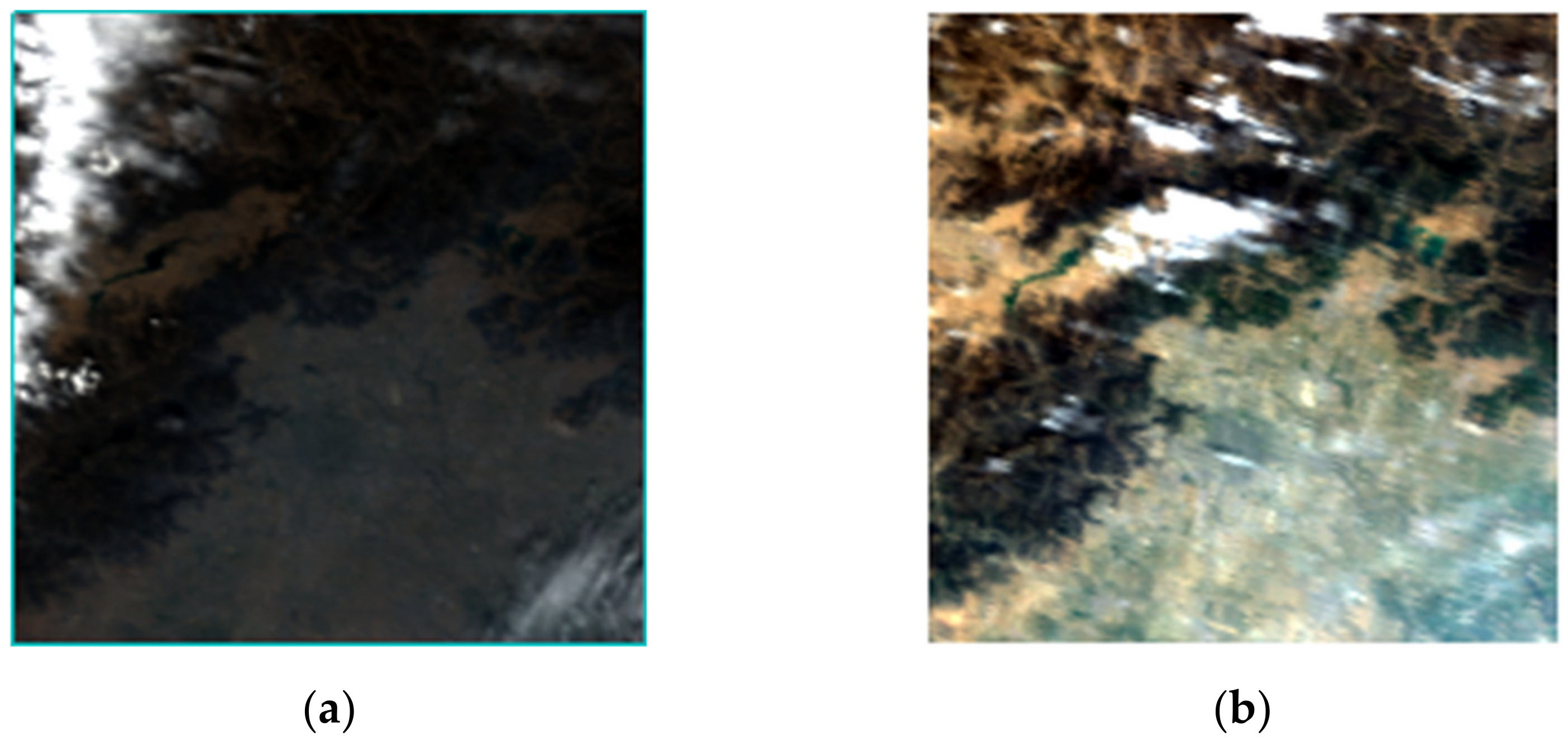
Table 1. We want to convert the satellite image into a three-channel RGB image to the convolutional neural network. Combining the wavelength range of visible light, as shown in
Table 2, the three channels that best fit the three bands of RGB are channel 1, channel 4, and channel 3, so we combine the data of these three channels to get a true-color image. The synthesized image is shown in
Figure 4. The correspondence AQI and PM 2.5 concentration of each haze level is shown in
Table 3.
4.2. CNN Structure
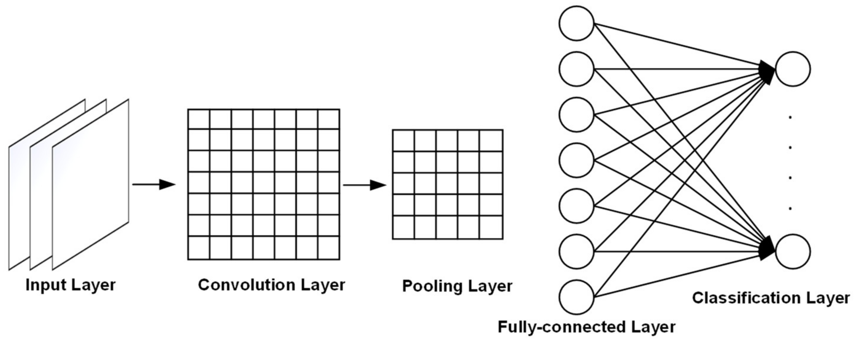
The general structure of the CNN network proposed in this article is shown in
Figure 5.
Input layer: If the input data are RGB true-color images, the input data format is: ; if they are grayscale image data, the input data format is: . Moreover, the input data of the input layer should be normalized, and the size of the image and the number of data channels should be consistent.
Convolution layer: The convolution operation is expressed as C, where f represents the length and width of the convolution kernel. The length and width are the same, and the number of channels is the same as the number of input channels. m represents the number of convolution kernels. Then, the process of convolution operation is shown in Equation (2):
The first-level summation formula means that all convolution kernels are traversed once. The second- and third-layer summation formulas indicate that a convolution kernel with a size of
is used to perform a convolution operation on the input, where W is the weight and
is the bias. Where
represent the position of the image in the output layer as shown in Equation (3):
Activation function: Use Sigmoid activation function, as shown in Equation (4):
Pooling layer: This is an essential step in a convolutional neural network, also called a down-sampling layer, and the size is generally a square window with the same length and width. The pooling process is shown in Equation (5):
After the input data are translated and transformed, the output will not change, improving the convolutional network’s robustness to extract features. This kind of translation invariance is a very practical property.
Fully connected layer: In the studied model, there are six categories according to the level of haze, and the corresponding labels are: (0 0 0 0 0 0 1), (0 0 0 0 0 1 0), ..., (0 1 0 0 0 0 0). Among them, data that are disturbed by information such as clouds and cannot be identified are marked with position 1, that is, (1 0 0 0 0 0 0).
SoftMax classification layer: The classification process is to judge the probability that this vector belongs to each category, and the one with the highest probability is the result of the classification, as shown in Equation (6):
where
represents the probability estimation of the classification function to the data being the nth category, and
represents the model’s parameters. The rightmost formula of the equation represents the normalized form of the probability so that the sum of all the probabilities is 1.
4.3. CNN Parameter Adjustment
We used the stochastic gradient descent method as the parameter adjustment optimization method. Although the convolutional neural network used in this article does not have many layers, its structure belongs to deep learning. Let θ be a parameter in the neural network, the negative conditional log-likelihood of the training data can be expressed by Equation (7):
where
represents the loss function corresponding to the
input, then for these cost functions that you want to add, the gradient descent method needs to be calculated using Equation (8):
The calculation time complexity of this optimization process is
, where m is the amount of data in the training set. As training increases, this complexity will increase. The core of the stochastic gradient descent method is to perform a small-scale sample approximate estimation. A small batch of training (minibatch) was performed in each step, and the sample size at this time was
, and
, and then pass. The results obtained in this part were used to estimate the results of the entire sample so that the amount of calculation will be significantly reduced. The gradient estimation, Equation (9), is as follows:
Use the mini-batch described above to train and estimate the entire sample using the following gradient estimation algorithm as Equation (10):
The small-batch gradient descent method solves the shortcomings of the gradient descent method’s time complexity and unreliability of the gradient descent method in the parameter optimization process. Finally, we optimized the parameters of the classification layer and used the evaluation function as Equation (11):
The optimization process is the process of minimizing the evaluation function so that the parameter will reach the optimal value.
5. Experiment and Result
5.1. Correlation Analysis between Traditional Method Inversion Results and Haze Concentration
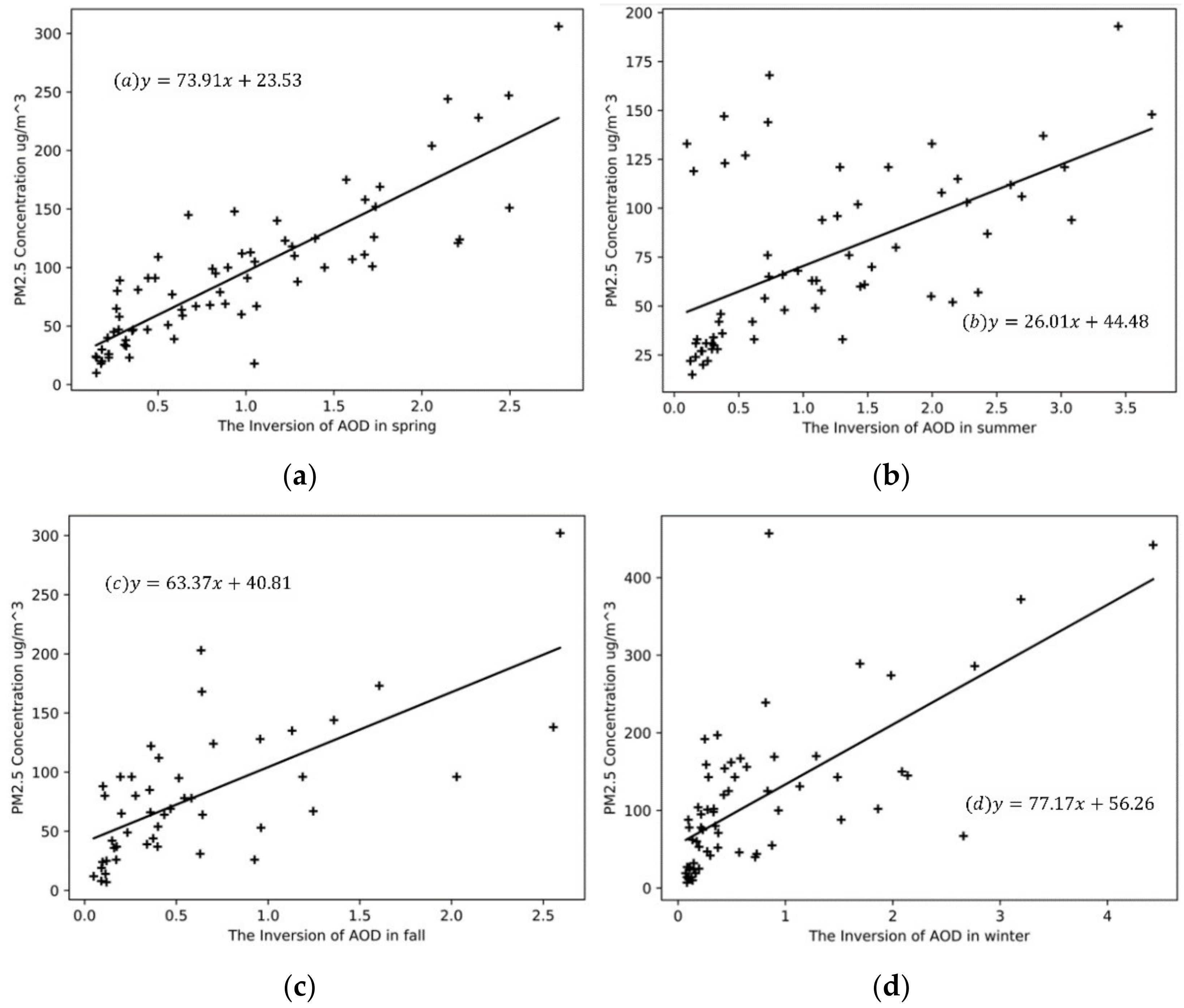
This experiment used traditional methods to analyze the correlation between the inversion data of MOD02-1 km in Beijing in 2014 and the PM2.5 concentration of ground monitoring stations in Beijing. The result is shown in
Figure 6, where (a–d) represents the results of the four seasons.
From the results, the highest correlation coefficient is in the spring inversion, which reaches a high level of 0.86, followed by winter and autumn, and the worst in summer. All of the correlation coefficients are above 0.5, indicating a strong correlation between AOD and PM2.5 concentration, considering their non-linear relationship and complex dynamics.
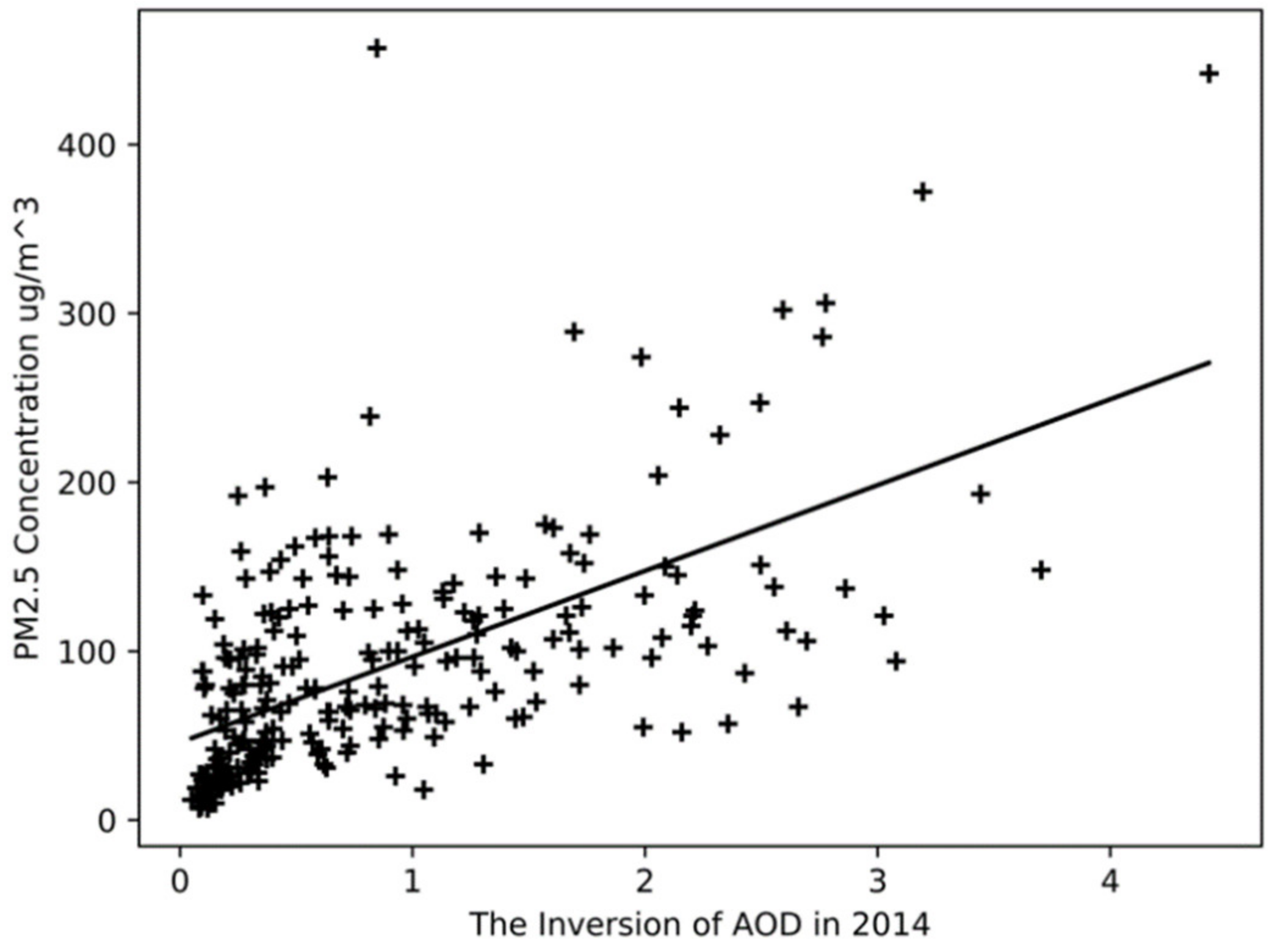
We also performed a linear fit to the inversion results of AOD in the whole year of 2014, as shown in
Figure 7. The y-intercept
is 45.85, the slope
is 50.79, and the correlation coefficient R is 0.59. Compared with the results of the four seasons, the correlation coefficient of the linear fit for the whole year is 30% lower than that of the spring. We think this is because the four seasons have different factors, such as different climatic characteristics, industrial activities, and gas emissions caused by heating demand, which contribute to the correlation between AOD and PM2.5 concentration. Therefore, we conclude that studying the correlation performance of AOD and PM2.5 according to the season division can provide a more accurate basis for analysis.
Figure 7 shows that we can train the processed data through the neural network method to approximate the coupling relationship between the mapping relation and the linear relation to achieve the inversion classification method.
5.2. Comparison of CNN Analysis Results
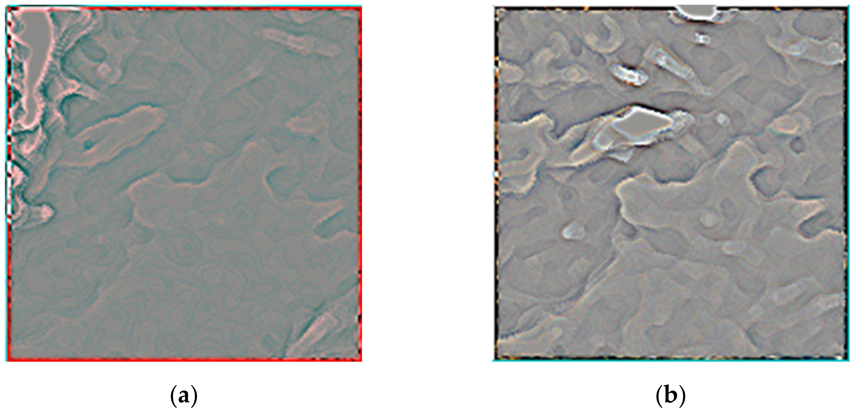
We extracted the image after two 7 × 7 convolution layers to analyze whether the model can extract the haze characteristics [
30,
31,
32], as shown in
Figure 8.
Figure 8a is a convolution result diagram when the haze is severe in spring, and the bright block is in the upper left corner of the image. We find a cloud layer in the area comparing it with the original image, which indicates that the cloud layer appears bright in the convolution result. The remaining areas with severe haze are darker, where the difference between emissivity and reflectance is more significant.
Figure 8b is a convolution result graph containing minimum cloud information and a lower haze concentration level. The brighter feature in
Figure 8 is the area where the AOD is low. The difference between the emissivity and the reflectance is slight. We found that the haze level prediction model can effectively distinguish the image characteristics of different haze concentrations by comparing the results. We labeled the cloud information of the image when marking the dataset, avoiding the mistakes where the cloud was identified as haze.
We used the MOD02-1 km data of the Beijing area in 2013 and 2014 as the training set and test set of the haze level prediction model. We extracted satellite images from the MOD02-1 km data so that the training and test sets contained 730 satellite images. We marked the haze level on the training set.
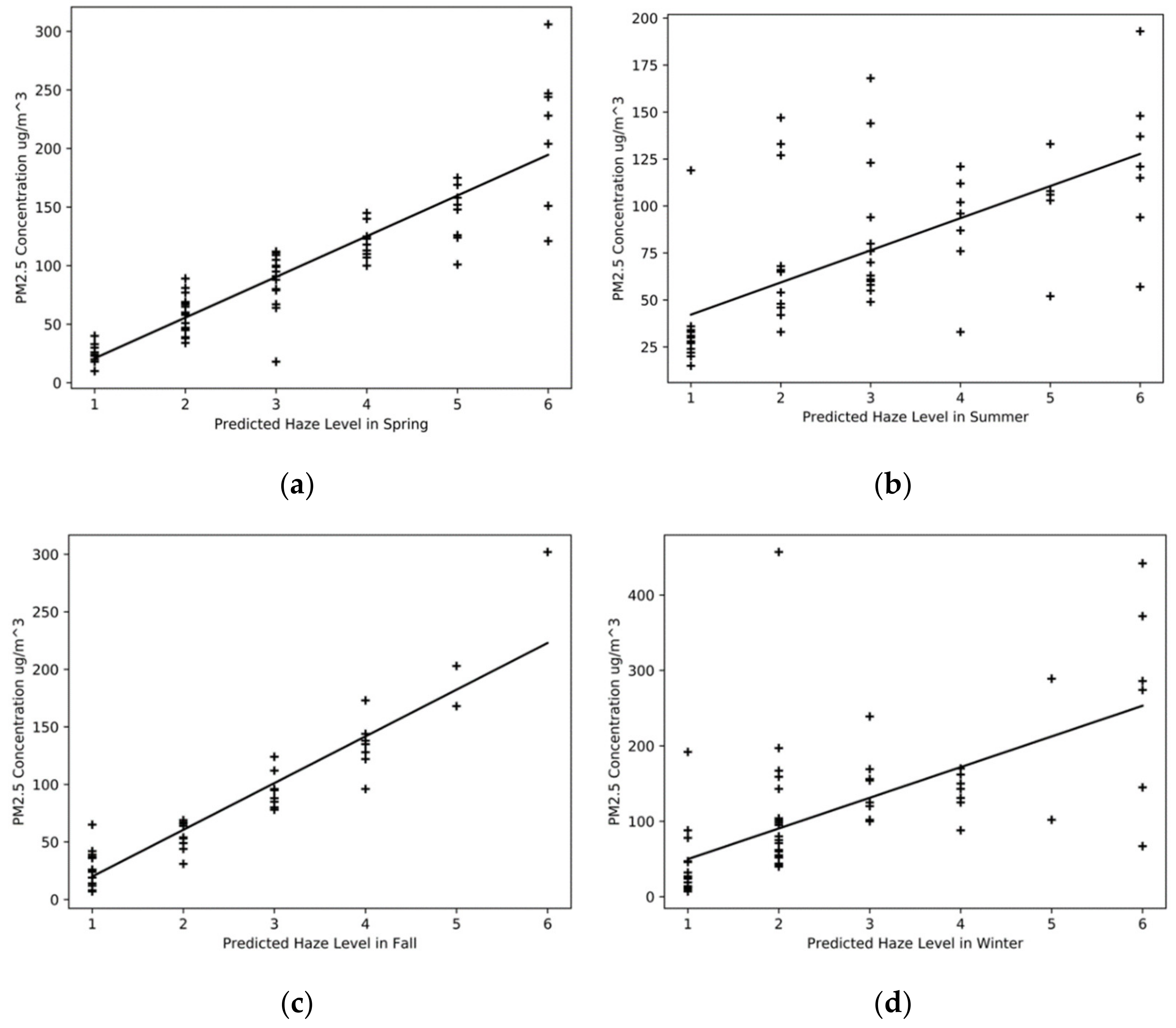
To verify whether the model can effectively establish the correlation between satellite image and PM2.5 concentration and to compare it with the traditional inversion method, we conducted the same linear regression between the output of the haze level prediction model and the PM2.5 daily average concentration. The results are shown in
Figure 9.
In
Figure 9a, the y-intercept
is −13.88. The slope
is 34.74. The correlation coefficient R is 0.90. In
Figure 9b, the y-intercept
is 25.07. The slope
is 17.11, and the correlation coefficient R is 0.65. In
Figure 9c, the y-intercept
is −20.74. The slope
is 40.61. The correlation coefficient R is 0.93. In
Figure 9d, the y-intercept
is 9.03, and the slope
is 40.67, the correlation coefficient R is 0.65.
A comparison with the traditional inversion method is shown in
Table 4.
From
Table 4, the correlation coefficient of the haze level prediction model based on the convolutional neural network is superior to the traditional inversion method in spring, summer, and fall. In particular, the summer and fall results are improved by 12% and 39%, respectively, which indicates that the haze level prediction model can provide a better PM2.5 concentration prediction than the traditional inversion method. Furthermore, all correlation coefficients in the haze prediction model are above 0.6, indicating a strong correlation between haze level and PM2.5 concentration.
6. Discussion
This study first studied the traditional haze inversion method. After studying the relationship between AOD and haze concentration, we found a non-linear mapping relationship between the two. Therefore, we propose a CNN-based haze classification model to take advantage of CNN’s non-linear relationship fitting. Through the experimental comparison between the traditional method and our proposed model, the correlation coefficient of the haze classification model based on the convolutional neural network in spring, summer and fall are better than the traditional inversion method. In particular, the results in summer and fall increased by 12% and 39%, respectively, which indicates that the CNN haze classification model can provide better classification results than traditional inversion methods. In addition, all correlation coefficients in the haze classification model are above 0.6, indicating a strong correlation between the haze level and the PM2.5 concentration.
In general, whether it is a traditional inversion method or a CNN-based method, summer has the lowest correlation coefficient, followed by winter. The reason may be that the fog concentration of summer aerosol is higher than that of haze. In winter, there are many days of heavy haze and uneven distribution of time and space, resulting in a low recognition rate of the CNN. On the other hand, the increase in fall is due to the smaller haze level, which is most concentrated in the top four levels, and there is less severe haze weather.
The result shows consistency with other studies [
3,
5,
20]. The winter is the most polluted season in this area of China. The pattern may contribute to the high correlation coefficient in the winter. The result from the CNN shows a better performance in spring, summer, and fall. The feature capture characteristics of the CNN and its ability to fit with complex functions could benefit haze classification and prediction [
31,
32]. Since the CNN model could improve the inversion results when the haze is less severe, other machine learning methods could be used on a broader range of areas and haze scenarios. After considering the limitations of both the proposed method and the comparison traditional method, the result of both the proposed method and the comparing result is limited. However, the results still show the potential of combining neural networks with time-consuming tasks in atmospheric studies.
7. Conclusions
This research is based on experimental research on convolutional neural networks’ classification and prediction of haze levels. We found that a convolutional neural network uses images to identify haze concentrations, which can sufficiently fit the non-linear relationship between input and output. It proves the feasibility of a convolutional neural network to classify and invert haze. At the same time, the use of trained convolutional neural networks can reduce manual inversion work to a certain extent. Our proposed CNN-based haze level classification model greatly simplifies data processing compared to traditional inversion methods. By comparing the correlation coefficients of traditional inversion methods and CNN-based methods, we prove that the haze prediction network can provide better PM2.5 concentration classification than traditional inversion methods. It also proves that the original remote sensing satellite images can provide rich features for analyzing haze problems.
Since this study still contains many limitations, including the limited data and only covering a limited range of the haze problem, this method is only the starting point for further combining machine learning methods with atmospheric problems. Moreover, the recognition rate reached more than 80%. However, due to insufficient data, the accuracy of the recognition result is not high, but it is also feasible. Among them, the accuracy rate and the F1 value of levels 1–4 are higher. However, the values of these three items of grades 5 and 6 all decreased, and the reason is because the concentration span of the latter two grades is larger.
Since the proposed method aims to replace and replicate the traditional process using CNN, the proposed method shares the same limitations as the traditional method. The estimate heavily depends on the satellite image, which contains many other elements that could be falsely claimed as haze. The traditional method uses various calibration processes with satellite parameters including azimuth, zenith, emissivity, and reflectivity to reduce these false results. Some of these calibration processes are removed to fit the network structure and simplify the network process when constructing a neural network to replace the labor-intensive traditional method. Although the proposed method has fewer calibrations and processes than the traditional method, the results are still compatible and even better than those in several situations. This result is likely caused by the nature of neural networks that have an outstanding performance in fitting complex natural processes. This study and previous studies have shown that neural networks have a great capacity and performance in simulating haze progress and in the prediction of haze states [
23,
24,
25,
26,
28,
31,
32]. Of course, due to all of the simplification processes, this study took some time to construct the network, and the original limitations of the traditional method still remain in the network, there will be many misfits and false claims of haze phenomena. In order to demonstrate the great potential of the neural network on the haze problem, we believe that the following aspects can be further studied to improve the accuracy of haze prediction.
Future studies could further improve the model’s ability to interpret images. In order to avoid the influence of clouds on the model’s ability to identify polluted areas and pollutant concentrations, this paper manually annotated cloud information on all satellite images. This paper also removed some steps in traditional image processing to reduce complexity and time, which would cause errors in the outcome. In future research, the model’s ability to process images can be improved to replace manual marking, which keeps the accuracy and quality. In addition, convolutional neural networks have good recognition performance for images, but they lack the ability to process time-series information. Therefore, to obtain the haze characteristics in the time series, utilizing more network models would benefit future studies.


 ,
, 


