Classification of Urban Pollution Levels Based on Clustering and Spatial Statistics

Abstract

In recent years, the occurrence and frequency of haze are constantly increasing, severely threatening people’s daily lives and health and bringing enormous losses to the economy. To this end, we used cluster analysis and spatial autocorrelation methods to discuss the spatial and temporal distribution characteristics of severe haze in China and to classify regions of China. Furthermore, we analyzed the interaction between haze pollution and the influence of economy and energy structure in 31 provinces in China, providing references for the prevention and treatment of haze pollution. The processed data mainly include API, meteorological station data, and PM 2.5 concentration distribution vector graph. The results show the yearly haze pattern from 2008 to 2012, and present a strong pattern of pollution concentrated around Beijing–Tianjin, the Yangtze River Delta, southwest China, and central China. The overall spatial pattern of decreasing from north to south is relatively constant over the study period.

1. Introduction

Alongside the development of the society and a growing economy from industrialization [1,2,3,4], various factors, such as rapid increases in population and the number of motor vehicles, have resulted in severe air pollution in some cities [5,6,7,8]. Since the beginning of the 21st century, severe air pollution has occurred in many countries, and haze is a typical weather situation [9,10,11]. The frequent occurrence of the haze phenomenon is closely related to aerosol pollution resulting from human activities. Aerosol particles in the air can absorb or scatter solar radiation, reducing visibility and facilitating haze conditions. In modern society, the severity of haze has attracted the attention of many different parts of society, including the general public and the scientific community; it is presently a “hot topic” [12,13,14].

Many scholars have studied the climate characteristics of haze weather. For example, Wu, who investigated the time and space distribution of haze in China, simulated the trend in the changes in haze over time, and then performed a detailed analysis to find out the cause of changes in haze and the relationship between the length of sunshine and solar radiation [15]. Wu, D. [16], according to the collection of data on haze from China’s 721 weather stations over 55 years (1951–2005), studied the time and space distribution of haze in mainland China. The results show that south of 42° N and east of 100° E is the gathering place for haze in China. On the whole, the volatility of haze is relatively frequent.

Other scholars researched the physical and chemical characteristics of aerosol in haze. For example, Yang Jun et al. [17] divided aerosols at different stages according to visibility and relative humidity and then discussed and studied the microphysical properties of aerosols at different stages. They found that the temporal variation in aerosol number concentration was negatively correlated with the average root diameter. According to the collected one-year ${\mathrm{PM}}_{2.5}$ concentrations, Zhao, P. et al. [18] studied the impact of the concentration of black carbon aerosol and meteorological data from observation sites on pollution in Tianjin city. The results show that the weather changes in Tianjin are closely related to the concentration of black carbon aerosols and that the concentration of black carbon in the air is relatively high during haze. Li Fei et al. [19] analyzed the typical haze day process in Guangzhou, mainly the characteristics of aerosol particles in the process. The results showed that the ${\mathrm{PM}}_{2.5}$ concentration and the black carbon concentration in the haze process reached 1902.7 $\mathsf{\mu }\mathrm{g}/{\mathrm{m}}^3$ and 355.7 $\mathsf{\mu }\mathrm{g}/{\mathrm{m}}^3$, respectively. Xu Zheng et al. [20] observed Jinan meteorology from an optical perspective. Their results showed that the scattering coefficient and aerosol absorption coefficient were relatively high on haze days, 2.6 and 2.8 times those on non-haze days, respectively. Giri, B. et al. [21] studied the composition and origin of aerosol particles in industrial areas of central India. The results show that the primary sources of organic tracers in aerosol PM in central India are fossil fuel products and biomass/waste combustion. The tracers contain low levels of organic compounds that exist in the natural background.

Spatial statistics have a wide range of applications in academic research. Among these, the ArcGIS developed by ERSI (located at Redlands, CA, USA) combined is favored by scientists when studying the spatial and temporal distribution characteristics of haze. Wei J. et al. [22] analyzed the temporal and spatial distribution characteristics of haze in Jiangsu and the impact of urbanization speed on the frequency of haze occurrence, using meteorological data and relevant economic statistical data. The results show that the probability of haze in southern Jiangsu has increased with the decrease in greening in the past 8 years, which indicates that the city’s rapid development is at the expense of an increased frequency of haze days. Spatial statistics offer great advantages in the study of data with spatial attributes and can obtain results that classical statistics do not allow from the perspective of spatial attributes [23]. At present, scholars at home and abroad have made some achievements in haze spatial statistics. The use and accuracy of spatial statistics are also improving owing to data processing and deep learning [24,25,26,27,28].

So far, most studies on haze have focused on the temporal and spatial distribution of haze in a specific city or region. However, there are far fewer studies on the temporal and spatial distribution of haze in the whole country in comparison. This paper analyzes air pollution data from Chinese meteorological stations, mainly from a statistical perspective, to study the spatial–temporal distribution of haze, associated impact factors, and air pollution in China.

2. Research area and Data Preprocessing

2.1. Research Area

The data range in this paper is from 1 January 2008 to 31 December 2012. It mainly contains the daily air pollution data of more than 120 cities in China during this period. The source of the data is the Ministry of Environmental Protection [29]. The data mainly include the city’s Air Pollution Index (API), air quality level, primary pollutant, and air quality status. Among the obtained data, there are more than 200 cities with a pollution index, but there are 86 city stations with data from January 2008 to 2012. Therefore, this paper used the data from 86 stations from 2008 to 2012 for the study. The above pollutant data are from https://www.aqistudy.cn/historydata/, accessed on 16 May 2019. The detected data include PM2.5, PM10, O₃, SO₂, CO, and NO₂. The units of PM2.5, PM10, O₃, and SO₂ are μg/m³; the units of CO and NO₂ are mg/m³.

There are many meteorological data stations in China, but they are not evenly distributed. There are fewer meteorological data stations in the peripheral areas, with greater density in the central area. The selected sites are generally distributed across the whole of China, but some regions do not have data in this period, including Henan, Jiangxi, and Shanghai. The location of data stations in each province is not uniform, but the whole region can be represented by interpolation. In order to display the station locations, the distribution of the data sites on a map is shown Figure 1.

Since the original data exist in the form of text, the meteorological station should be analyzed as a spatial object in the study, which requires preliminary data processing after obtaining the primary data are obtained. First, the data should be vectorized according to the longitude and latitude of the earthquake to generate the spatial point data. The data were then imported into ArcGIS, and, for this paper, the coordinate system was set as the WGS1984 coordinate system.

2.2. Pollution Data Processing

The clustering indices we chose were API, primary pollutant, and air quality level, respectively. After the selected data are obtained and imported as described above, the data need to be normalized so that the data values are between 0 and 1 to obtain good clustering results. The normalization equation is shown below:

$$\overline{X_{ij}}=\left(x_{ij}-min(x_j\right))/\left(max(x_j\right)-min(x_j))$$

(1)

where $\overline{X_{ij}}$ is the data obtained through normalization in the i-th row and the j-th column, and ${\mathrm{x}}_{ij}$ is the data belonging to the i-th row and the j-th column in the original data.

In order to further observe its clustering effect, the annual data were analyzed by clustering. After many experiments, the clustering result was better when the k value reached 4, and the spatial boundary was the clearest. Because we are trying to find out the spatial and temporal characteristics of the clustering results, we focus on the characteristics of cities in different spaces or the clustering results over time. After the completion of clustering, different city points will be divided into different categories, and each city has an additional attribute of a category.

3. Methods

Cluster analysis mainly refers to the grouping of research objects. The basis of grouping is that the attributes of the research objects are relatively similar, and that similar groups are divided according to the overall attributes. From the perspective of statistics alone, cluster analysis can be understood as the simplification of data and the simple classification of data according to the model [30]. On the other hand, systematic cluster analysis is traditional statistical cluster analysis, which is a classification method to analyze the research objects comprehensively from multiple perspectives. Various types of statistical analysis software are available, such as SPSS and SAS. This paper uses SPSS to perform systematic cluster analysis on the research data.

The systematic cluster analysis is used to classify the elements in the study according to different classification purposes based on the prior statistical geographical data. The process of systematic clustering can be divided into several steps.

Step 1 is processing the clustering elements. Since statistical data generally consist of multiple attributes, the dimensions and units of different attributes are different. The results of such classification will cause inaccurate classification results due to large differences between the data, so the data must be processed first before classification. Common processing methods include sum standardization, standard deviation standardization, maximum value standardization, and difference standardization [29,31,32]. The most common application is standard deviation standardization. The standard deviation standardization process used is given below:

$$x_{ij}^{\prime }=\frac{x_{ij}-\overline{x_j}}{s_j}\hspace{1em}i=1,2,\cdots ,n;j=1,2,\cdots ,m$$

(2)

where $\overline{x_j}=\frac{1}{n}\sum _{i=1}^n{x}_{ij}$, $s_j^2=\frac{1}{n-1}\sum _{i=1}^n{\left(x_{ij}-\overline{x_j}\right)}^2$, when $j=1,2,\cdots ,m$. After this process, the mean of each of these variables is 0, the standard deviation is 1, and the impact of the units on the data and the dimensions are removed.

Step 2: Calculate the distance between samples: Select the appropriate distance to measure the distance between any two samples and obtain the sample distance matrix $D^{\left(0\right)}$.

Step 3: Clustering process: Before classification, each sample studied was separately regarded as a class, and the number of classifications was $k=n$:$G_i=\left\{X_{\left(i\right)}\right\}\left(i=1,2,\cdots ,n\right)$. At this time, the distance between classes and samples is equivalent, namely, $D^{\left(1\right)}=D^{\left(0\right)}$. After that, let $j=1,2,\cdots ,n$, and the combination of sample classes is completed according to the following procedure:

(1)

Combine the two classes with the smallest distance into one. At this time, the number of classes divided into samples decreases by 1 on the original basis. The number of classes at this time is K = n − j + 1;

(2)

Calculate the distance between the new class and the remaining class, and then obtain the new distance matrix $D^{\left(j\right)}$.

If the class is merged k > 1, repeat steps (1) and (2) until k = 1.

Step 4: Draw a genealogical clustering diagram: the genealogical clustering diagram shows that the samples are classified as a whole in different clustering stages and the merging relationship among them.

Step 5: Determine the number of classes and the number of classes that contain members.

By finding out the indicator statistics, this paper can measure the similarity of the statistical data. Then, the selected statistics are used to classify the research object categories. Finally, a pedigree diagram can be drawn according to the distance relationship between classes. The samples contained in each class at each step will be presented from the pedigree diagram. Systematic cluster analysis is based on the largest difference between classes and the smallest difference between members within a class presented through the pedigree diagram.

4. Experiment and Result Analysis

4.1. Cluster Analysis

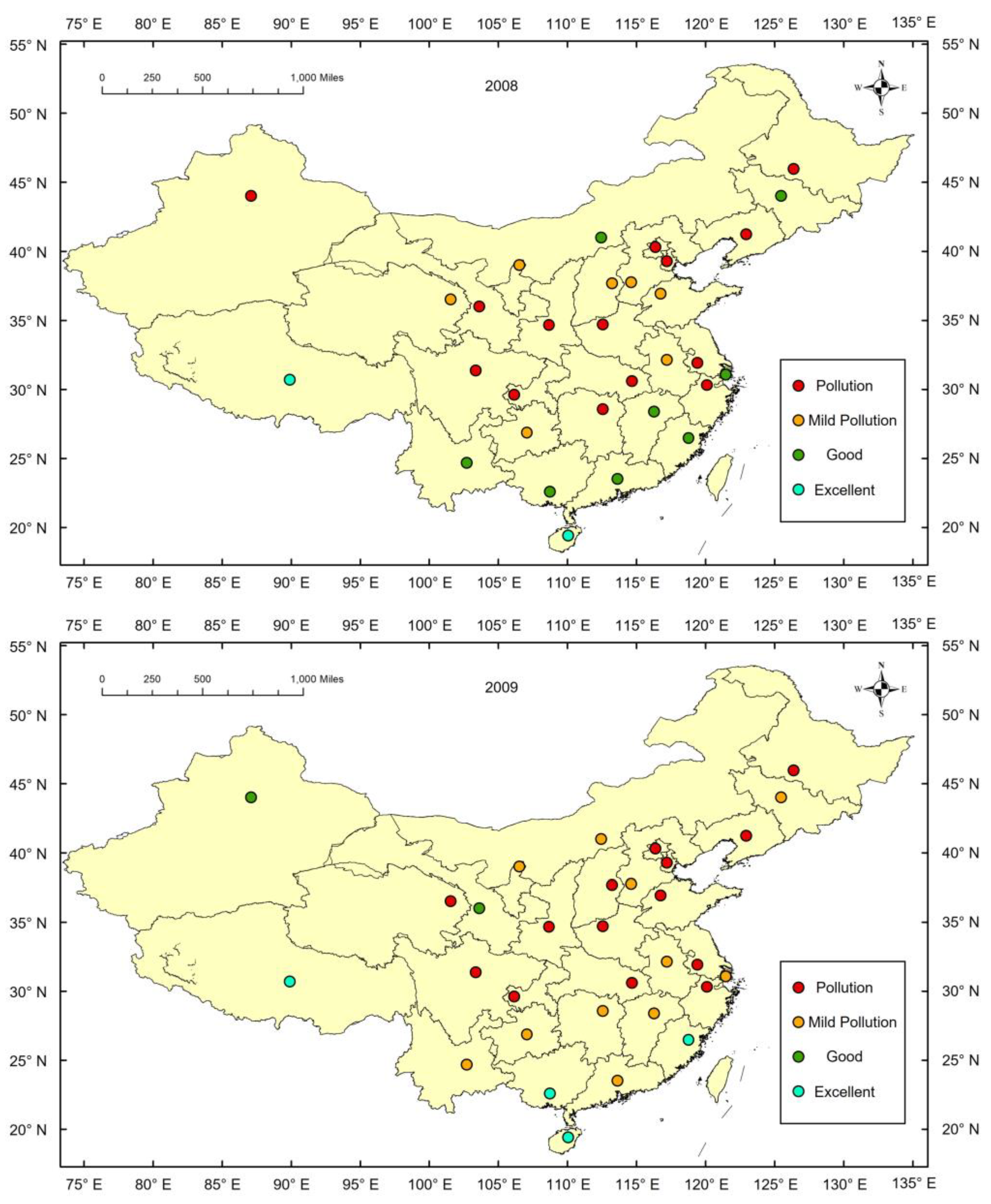
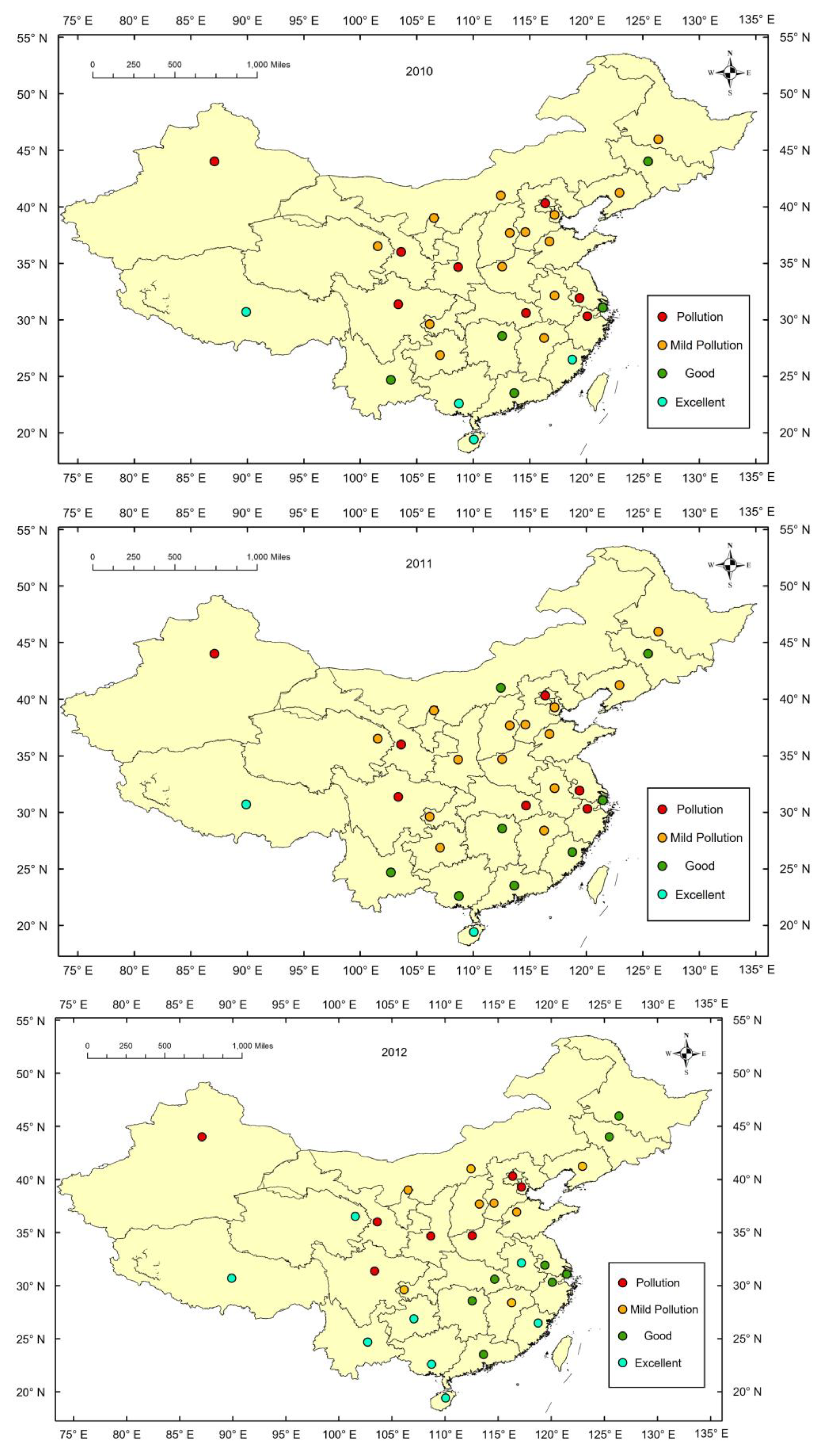
According to the number of clusters divided into groups to study the situation of each region, the spatial coverage of each region (including the cities) is counted. Then, the API of the classified cities is analyzed, which is helpful to discover the commonness of regional pollution. In the analysis of the classification of cities from 2008 to 2012, the data were also divided into four categories: polluted, slightly polluted, good, and excellent. The main factors to be considered are the concentration of SO, NO, and PM. According to the concentration of these three, the cluster analysis of the provincial capital city is performed. In order to see the pollution classification of each provincial capital city studied, we generated a detailed explanation from the spatial location distribution and specific classification.

Figure 2 shows the pollution classification of provincial capital cities from 2008 to 2012. A point represents each provincial capital city, and points are given different colors according to the pollution situation of different cities. Red, yellow, green, and blue represent pollution, mild pollution, good, and excellent, respectively.

Table 1. Clustering results in 2008.

2008	Included City	Type	Proportion
First	Beijing, Chengdu, Harbin, Hangzhou, Jinan, Lanzhou, Nanjing, Shenyang, Shijiazhuang, Taiyuan, Tianjin, Urumqi, Wuhan, Xi’an, Changsha, Zhengzhou, Chongqing	Pollution	54.8%
Second	Fuzhou, Guangzhou, Hohhot, Kunming, Nanning, Shanghai	Light pollution	19.4%
Third	Guiyang, Hefei, Nanchang, Xining, Yinchuan, and Changchun	Good	19.4%
Fourth	Haikou, Lhasa	Optimal	6.5%

,

Table 2. Clustering results in 2009.

2009	Included City	Type	Proportion
First	Lanzhou, Urumqi	Pollution	6.5%
Second	Beijing, Chengdu, Harbin, Hangzhou, Jinan, Nanjing, Shenyang, Taiyuan, Tianjin, Wuhan, Xi’an, Xining, Zhengzhou, Chongqing	Light pollution	45.2%
Third	Guangzhou, Guiyang, Hefei, Hohhot, Kunming, Nanchang, Shanghai, Shijiazhuang, Yinchuan, Changchun, Changsha	Good	35.5%
Fourth	Fuzhou, Haikou, Lhasa, and Nanning	Optimal	12.9%

,

Table 3. Clustering results in 2010.

2010	Included City	Type	Proportion
First	Beijing, Chengdu, Hangzhou, Lanzhou, Nanjing, Urumqi, Wuhan, Xi’an	Pollution	25.8%
Second	Guiyang, Harbin, Hefei, Hohhot, Jinan, Nanchang, Shenyang, Shijiazhuang, Taiyuan, Tianjin, Xining, Yinchuan, Zhengzhou, Chongqing, Nanning	Light pollution	45.21
Third	Guangzhou, Kunming, Shanghai, Changchun, Changsha	Good	16.1%
Fourth	Fuzhou, Haikou, Lhasa, and Nanning	Optimal	2.9%

,

Table 4. Clustering results in 2011.

2011	Included City	Type	Proportion
First	Beijing, Chengdu, Hangzhou, Lanzhou, Nanjing, Urumqi, Wuhan	Pollution	22.6%
Second	Guiyang, Harbin, Hefei, Hohhot, Jinan, Nanchang, Shenyang, Shijiazhuang, Taiyuan, Tianjin, Xi’an, Xining, Yinchuan, Zhengzhou, Chongqing	Light pollution	48.4%
Third	Fuzhou, Guangzhou, Kunming, Nanning, Shanghai, Changchun, Changsha	Good	22.6%
Fourth	Haikou, Lhasa	Optimal	6.5%

and

Table 5. Clustering results in 2012.

2012	Included City	Type	Proportion
First	Beijing, Chengdu, Lanzhou, Tianjin, Urumqi, Xi’an, Zhengzhou	Pollution	22.6%
Second	Hohhot, Jinan, Nanchang, Shenyang, Shijiazhuang, Taiyuan, Yinchuan, Chongqing	Light pollution	25.8%
Third	Guangzhou, Harbin, Hangzhou, Nanjing, Shanghai, Wuhan, Changchun, Changsha	Good	25.8%
Fourth	Fuzhou, Guiyang, Haikou, Hefei, Kunming, Lhasa, Nanning, Xining	Optimal	25.8%

show the classification of each year. The yearly clustering results are grouped into a table.

From the spatial location of each pollution classification in Figure 2, the pollution status of each provincial capital city changes with time. However, the change in pollution status is relatively small, and the change in the category is relatively small. Most of the polluted and mildly polluted areas are concentrated in North China, Urumqi, and Hohhot. Areas with excellent air quality are mainly distributed in China’s coastal and marginal areas. The above is only a general introduction to the spatial classification. The distribution of cities in different years is given in Table 1, Table 2, Table 3, Table 4 and Table 5 to show the cities’ grades in more detail.

The clustering results of different years are different from the above tables, but the overall difference is not significant. Beijing, Chengdu, Lanzhou, and Harbin belong to the same category every year; all belong to the pollution category. Haikou and Lhasa are the two cities with better quality. Hefei, Shijiazhuang, Xi’an, Zhengzhou, and Chongqing are less polluted. Based on the results, this paper classified all cities into four groups shown in

Table 6. Overall clustering results in 2007–2012.

Overall Classification	Included City	Type	Proportion
First	Beijing, Chengdu, Ha’erbin, Hangzhou, Lanzhou, Nanjing, Urumqi, Wuhan	Pollution	25.8%
Second	Fuzhou, Guangzhou, Guiyang, Hohhot, Kunming, Nanchang, Nanning, Shanghai, Yinchuan, Changchun, Changsha	Good	35.5
Third	Haikou, Lhasa	Optimal	6.5%
Fourth	Hefei, Jinan, Shenyang, Shijiazhuang, Taiyuan, Tianjin, Xi’an, Xining, Zhengzhou, Chongqing	Light pollution	32.3%

. From the perspective of classification, by 2012, the proportions of all kinds of pollution were in a concentrated state, and the proportion was around 25%.

4.2. Spatial Statistical Analysis of Block Results

4.2.1. Distribution of Absorbable Particle Concentration

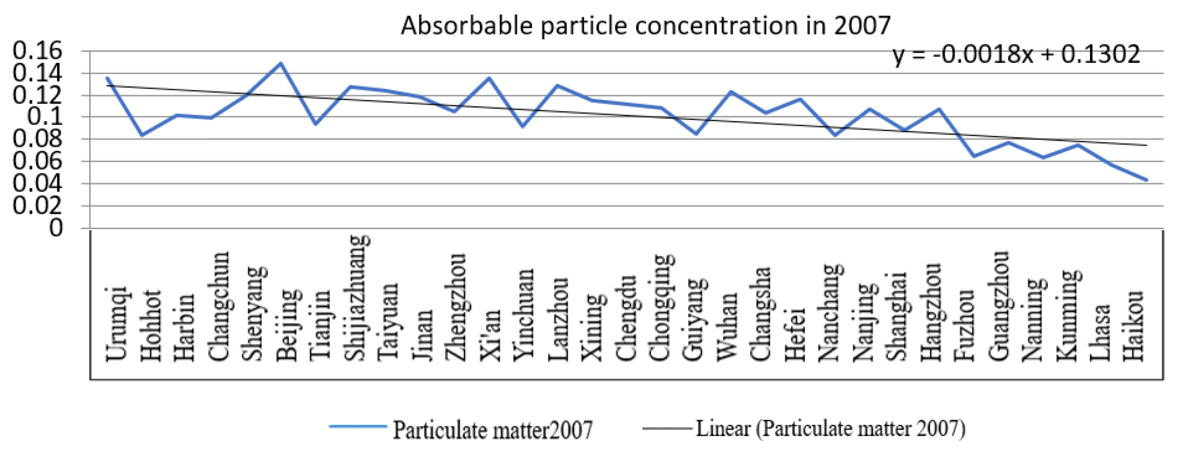
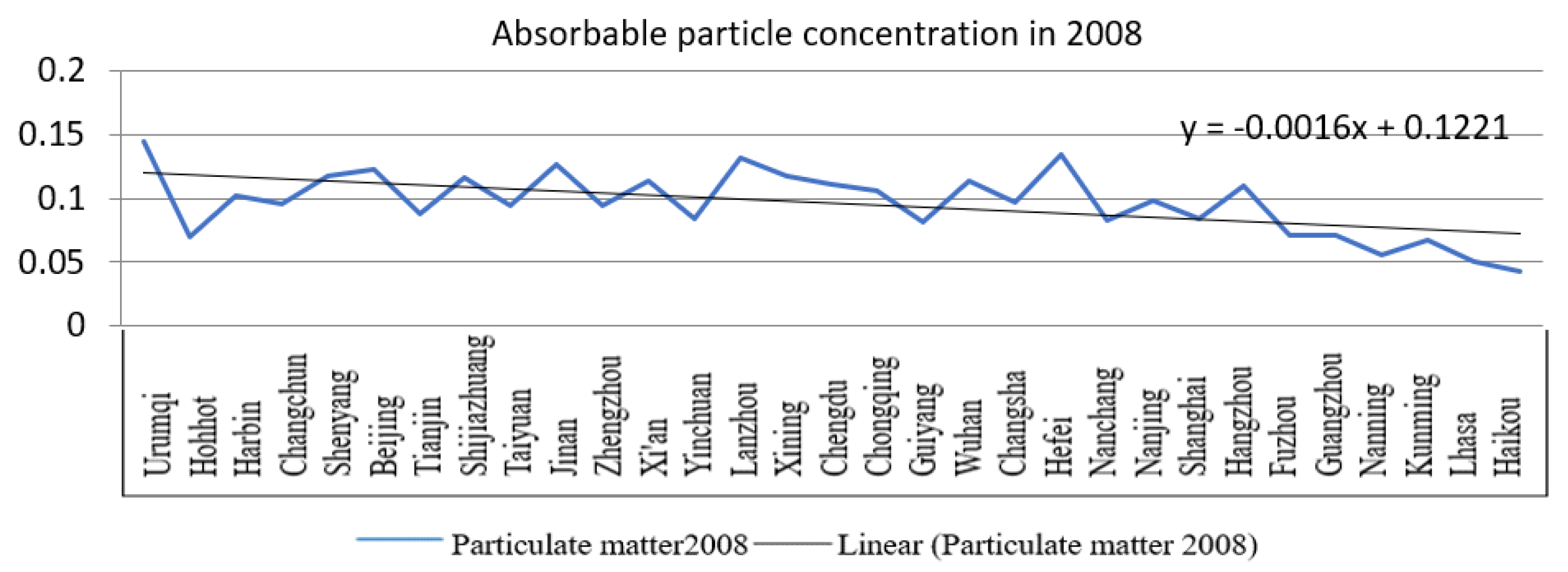
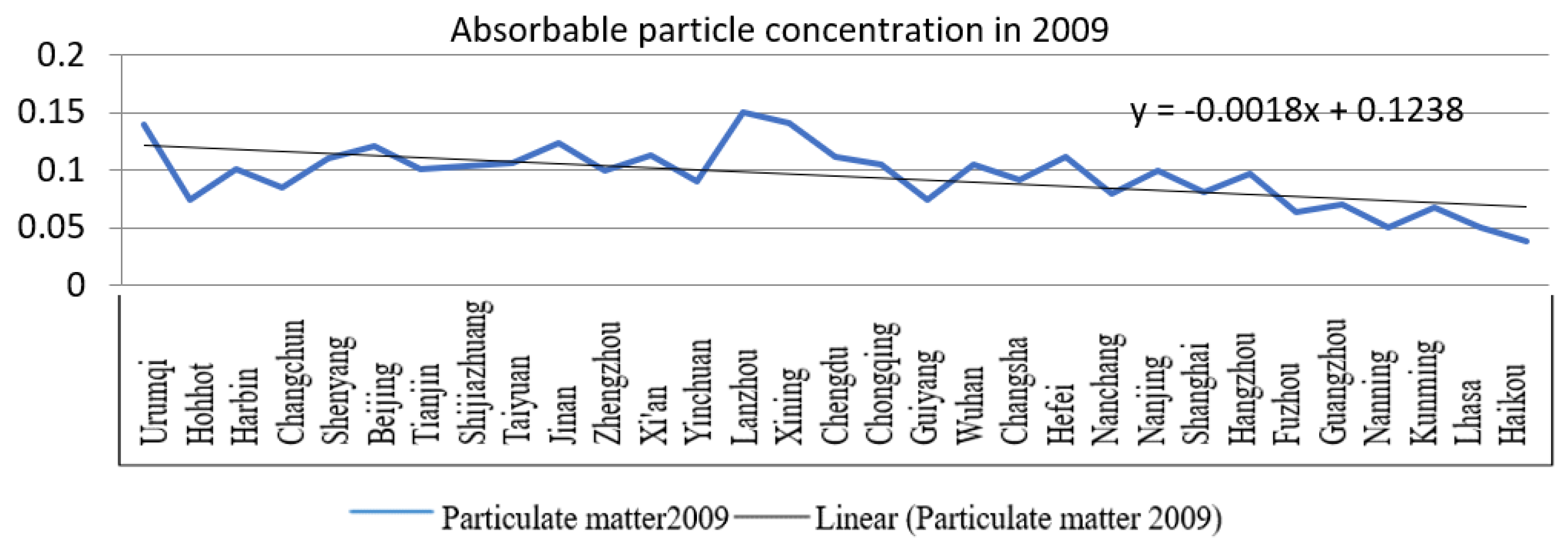
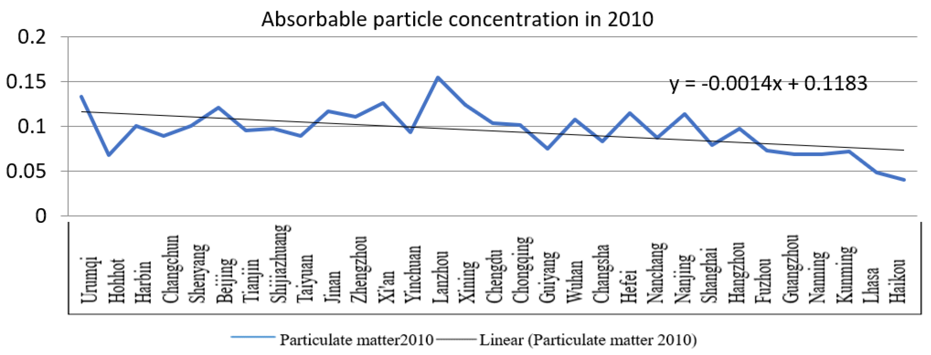
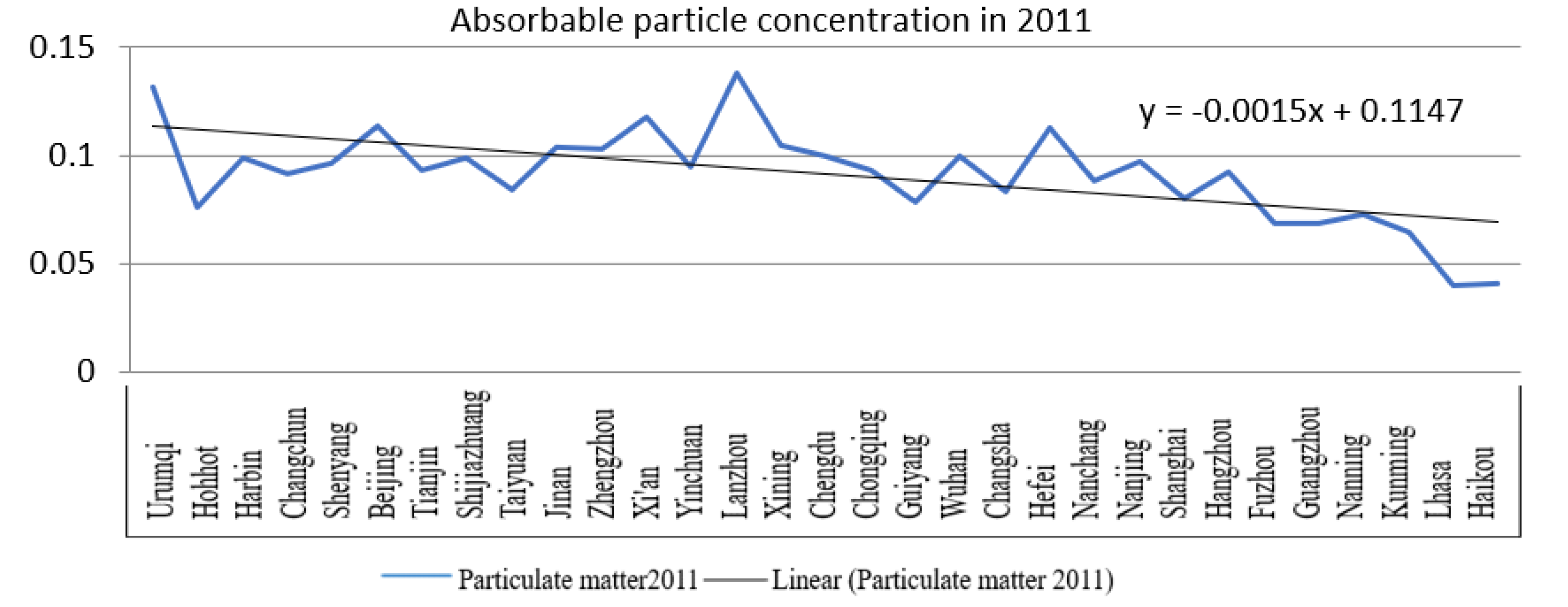
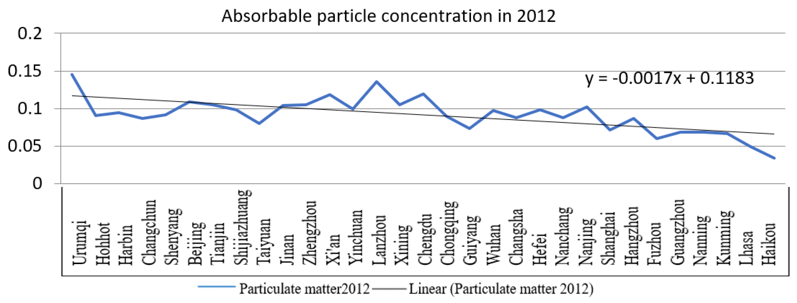
The hypothesis was that the mean concentration of absorbable particulate matter was relatively high in the middle part of China and relatively low in the coastal and marginal areas. Due to more rainfall and wind, absorbable particles cannot easily gather in coastal areas and are easily blown away by rain or wind. In order to prove our hypothesis, the line chart of the concentration of particulate matter from each provincial capital city is drawn in the order from north to south and from inland to coastal. The concentration of particulate matter can be absorbed after trend analysis. The diagram shows that each year, the trend in the figure, the slope, is negative, proving that the above hypothesis is correct. On the other hand, the slope from north to south and inland to coastal did not change much from the selected years of 2007 to 2012 as shown in Figure 3, Figure 4, Figure 5, Figure 6, Figure 7 and Figure 8.

4.2.2. China’s Regional Module Division

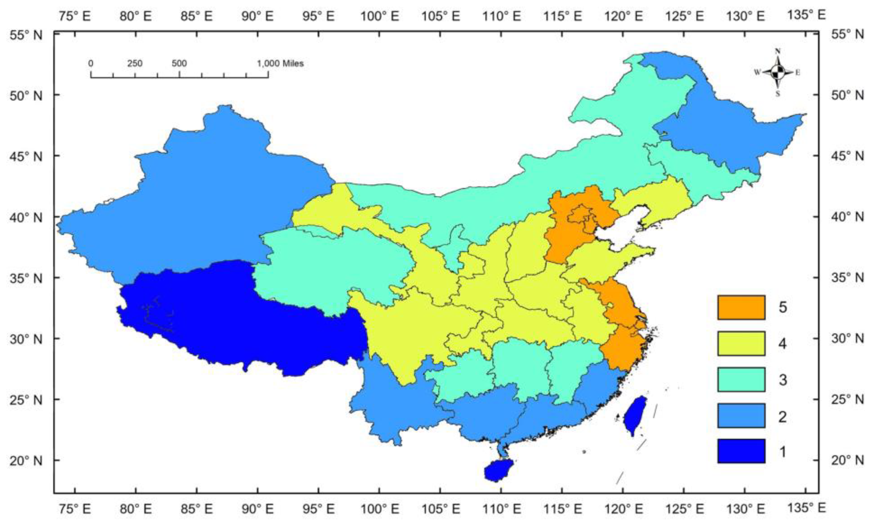
Based on the above analysis and considering the spatial correlation between each city and its surrounding cities under the PM2.5 index, 31 key cities are divided into the following blocks, as shown in the Figure 9.

The figure above shows that Region 1 includes heavily polluted cities, represented by Beijing, including Tianjin, Beijing, Hebei, Shanghai, Jiangsu, and Zhejiang. The above analysis results show that these areas are urban areas with high air pollution concentrations. Region 2 includes lightly polluted cities such as Henan, Shandong, Shaanxi, Hubei, Sichuan, Chongqing, Lanzhou, Shanxi, and Anhui. Region 3 includes Guizhou, Hunan, Jiangxi, Qinghai, Inner Mongolia, Jilin, and others. Region 4 includes the coastal cities of Yunnan, Guangxi, Guangdong, Fujian, and Liaoning. Finally, Region 5 includes Hainan and Xizang, cities with better air quality.

5. Discussion and Conclusions

With the aim of studying the spatial and temporal distribution of haze in China, this paper considers statistical perspectives using air pollution data from Chinese meteorological stations. This paper reveals the regional divisions in China, and has the following main conclusions:

The clustering results of the pollution index in different years are different. Some cities will have changes in different pollution levels in different years, but the general changes are not large. In particular, Beijing, Chengdu, Lanzhou, and Hangzhou have always been in the heavily polluted level for different years. Lhasa and Haikou are always at the excellent level. The remaining cities vary slightly between mildly polluted and good.

In China, the concentration of absorbable particles decreased from north to south, and the decreasing trend did not change much in different years. As a result, the slope of the trend line of absorbable particle concentration composed of cities from north to south was basically stable.

According to the above spatial positive correlation analysis and clustering results, China could be divided into five parts. The polluted areas are concentrated in the Beijing–Tianjin–Hebei region, the Yangtze River Delta region, southwest China, and central China. On the other hand, the good air quality areas are concentrated in Hainan and Xizang.

This paper started with meteorological data, but there are some deficiencies in the research. The analysis of the urban pollution index only contains published data from the environmental protection department of the People’s Republic of China. Some major cities do not have published data; thus, they are not counted in the study. The existing data are limited, so kriging interpolation is adopted using ArcGIS. Due to insufficient data from some cities, the final result images may be different from individual studies on each city. Based on these limitations, further improvements can be made in future studies. The statistics of the urban pollution index can be directly or indirectly collected from other sources instead of limited to published data by the governmental institute. For example, by bringing remote sensing data into the scope, the study of haze behavior in China can be explored further in the future.

References

- Zheng, W.; Li, X.; Lam, N.; Wang, D.; Yin, L.; Yin, Z. Impact of land use on urban water-logging disaster: A case study of Beijing and New York cities. Environ. Eng. Manag. J. 2017, 16, 1211–1216. [Google Scholar] [CrossRef]
- Zheng, W.; Li, X.; Yin, L.; Wang, Y. The Retrieved Urban LST in Beijing Based on TM, HJ-1B and MODIS. Arab. J. Sci. Eng. 2016, 41, 2325–2332. [Google Scholar] [CrossRef]
- Chen, X.; Yin, L.; Fan, Y.; Song, L.; Ji, T.; Liu, Y.; Tian, J.; Zheng, W. Temporal evolution characteristics of PM2.5 concentration based on continuous wavelet transform. Sci. Total Environ. 2020, 699, 134244. [Google Scholar] [CrossRef]
- Tang, Y.; Liu, S.; Li, X.; Fan, Y.; Deng, Y.; Liu, Y.; Yin, L. Earthquakes spatio–temporal distribution and fractal analysis in the Eurasian seismic belt. Rend. Lincei Sci. Fis. Nat. 2020, 31, 203–209. [Google Scholar] [CrossRef]
- Li, X.; Zheng, W.; Yin, L.; Yin, Z.; Song, L.; Tian, X. Influence of Social-economic Activities on Air Pollutants in Beijing, China. Open Geosci. 2017, 9, 314–321. [Google Scholar] [CrossRef] [Green Version]
- Maharjan, L.; Tripathee, L.; Kang, S.; Ambade, B.; Chen, P.; Zheng, H.; Li, Q.; Shrestha, K.L.; Sharma, C.M. Characteristics of Atmospheric Particle-bound Polycyclic Aromatic Compounds over the Himalayan Middle Hills: Implications for Sources and Health Risk Assessment. Asian J. Atmos. Environ. 2021, 15, 1–19. [Google Scholar] [CrossRef]
- Liu, Y.; Tian, J.; Zheng, W.; Yin, L. Spatial and temporal distribution characteristics of haze and pollution particles in China based on spatial statistics. Urban Clim. 2022, 41, 101031. [Google Scholar] [CrossRef]
- Zheng, W.; Li, X.; Xie, J.; Yin, L.; Wang, Y. Impact of human activities on haze in Beijing based on grey relational analysis. Rend. Lincei 2015, 26, 187–192. [Google Scholar] [CrossRef]
- Zheng, W.; Li, X.; Yin, L.; Wang, Y. Spatiotemporal heterogeneity of urban air pollution in China based on spatial analysis. Rend. Lincei 2016, 27, 351–356. [Google Scholar] [CrossRef]
- Ambade, B.; Kumar, A.; Latif, M. Emission Sources, Characteristics and Risk Assessment of Particulate Bound Polycyclic Aromatic Hydrocarbons (PAHs) from Traffic Sites. 2021. Available online: https://www.researchsquare.com/article/rs-328364/v1 (accessed on 17 May 2021).
- Kurwadkar, S.; Dane, J.; Kanel, S.R.; Nadagouda, M.N.; Cawdrey, R.W.; Ambade, B.; Struckhoff, G.C.; Wilkin, R. Per- and polyfluoroalkyl substances in water and wastewater: A critical review of their global occurrence and distribution. Sci. Total Environ. 2021, 809, 151003. [Google Scholar] [CrossRef]
- Ambade, B.; Sethi, S.S.; Giri, B.; Biswas, J.K.; Bauddh, K. Characterization, Behavior, and Risk Assessment of Polycyclic Aromatic Hydrocarbons (PAHs) in the Estuary Sediments. Bull. Environ. Contam. Toxicol. 2021, 108, 243–252. [Google Scholar] [CrossRef] [PubMed]
- Ambade, B.; Kumar, A.; Kumar, A.; Sahu, L.K. Temporal variability of atmospheric particulate-bound polycyclic aromatic hydrocarbons (PAHs) over central east India: Sources and carcinogenic risk assessment. Air Qual. Atmos. Health 2022, 15, 115–130. [Google Scholar] [CrossRef] [PubMed]
- Kumar, A.; Sankar, T.K.; Sethi, S.S.; Ambade, B. Characteristics, toxicity, source identification and seasonal variation of atmospheric polycyclic aromatic hydrocarbons over East India. Environ. Sci. Pollut. Res. 2020, 27, 678–690. [Google Scholar] [CrossRef]
- Wu, X.; Guo, J. Inputs Optimization to Reduce the Undesirable Outputs by Environmental Hazards: A DEA Model with Data of PM2.5 in China. In Economic Impacts and Emergency Management of Disasters in China; Springer: Singapore, 2021; pp. 547–580. [Google Scholar]
- Wu, D.; Wu, X.-J.; Li, F.; Tan, H.-B.; Chen, J.; Chen, H.-H.; Chen, H.-Z.; Cao, Z.-Q.; Li, H.-Y.; Sun, X. Long-term variations of fog and mist in mainland China during 1951–2005. J. Trop. Meteorol. 2013, 19, 181. [Google Scholar]
- Yang, J.; Niu, Z.-Q.; Shi, C.-E.; Liu, D.-Y.; Li, Z.-H. Microphysics of atmospheric aerosols during winter haze/fog events in Nanjing. Huan Jing Ke Xue 2010, 31, 1425–1431. [Google Scholar] [PubMed]
- Zhao, P.; Dong, F.; Yang, Y.; He, D.; Zhao, X.; Zhang, W.; Yao, Q.; Liu, H. Characteristics of carbonaceous aerosol in the region of Beijing, Tianjin, and Hebei, China. Atmos. Environ. 2013, 71, 389–398. [Google Scholar] [CrossRef]
- Li, F.; Wu, D.; Tan, H.; Bi, X.; Jiang, D.; Deng, T.; Chen, H.; Deng, X. The characteristics and causes analysis of a typical haze process during the dry season over Guangzhou area: A case study. J. Trop. Meteorol. 2012, 28, 113–122. [Google Scholar]
- Xu, Z.; Li, W.-J.; Yu, Y.-C.; Wang, X.-F.; Zhou, S.-Z.; Wang, W.-X. Characteristics of aerosol optical properties at haze and non-haze weather during autumn at Jinan city. China Environ. Sci. 2011, 31, 546–552. [Google Scholar]
- Giri, B.; Patel, K.S.; Jaiswal, N.K.; Sharma, S.; Ambade, B.; Wang, W.; Simonich, S.L.M.; Simoneit, B.R. Composition and sources of organic tracers in aerosol particles of industrial central India. Atmos. Res. 2013, 120–121, 312–324. [Google Scholar] [CrossRef] [Green Version]
- Wei, J.; Zhu, W.; Liu, D.; Han, X. The Temporal and Spatial Distribution of Hazy Days in Cities of Jiangsu Province China and an Analysis of Its Causes. Adv. Meteorol. 2016, 2016, 6761504. [Google Scholar] [CrossRef]
- Shang, K.; Chen, Z.; Liu, Z.; Song, L.; Zheng, W.; Yang, B.; Liu, S.; Yin, L. Haze Prediction Model Using Deep Recurrent Neural Network. Atmosphere 2021, 12, 1625. [Google Scholar] [CrossRef]
- Van Donkelaar, A.; Martin, R.V.; Park, R. Estimating ground-level PM2.5using aerosol optical depth determined from satellite remote sensing. J. Geophys. Res. Atmos. 2006, 111. [Google Scholar] [CrossRef]
- Liu, Y.; Sarnat, J.A.; Kilaru, V.; Jacob, D.J.; Koutrakis, P. Estimating Ground-Level PM2.5 in the Eastern United States Using Satellite Remote Sensing. Environ. Sci. Technol. 2005, 39, 3269–3278. [Google Scholar] [CrossRef] [PubMed] [Green Version]
- Wang, Z.; Chen, L.; Tao, J.; Zhang, Y.; Su, L. Satellite-based estimation of regional particulate matter (PM) in Beijing using vertical-and-RH correcting method. Remote Sens. Environ. 2010, 114, 50–63. [Google Scholar] [CrossRef]
- Ellrod, G.P. Advances in the Detection and Analysis of Fog at Night Using GOES Multispectral Infrared Imagery. Weather Forecast. 1995, 10, 606–619. [Google Scholar] [CrossRef] [Green Version]
- Guo, F.; Yang, B.; Zheng, W.; Liu, S. Power frequency estimation using sine filtering of optimal initial phase. Measurement 2021, 186, 110165. [Google Scholar] [CrossRef]
- Ye, S.; Ma, T.; Duan, F.; Li, H.; He, K.; Xia, J.; Yang, S.; Zhu, L.; Ma, Y.; Huang, T.; et al. Characteristics and formation mechanisms of winter haze in Changzhou, a highly polluted industrial city in the Yangtze River Delta, China. Environ. Pollut. 2019, 253, 377–383. [Google Scholar] [CrossRef] [PubMed]
- Stone, R.C. Weather types at Brisbane, Queensland: An example of the use of principal components and cluster analysis. Int. J. Clim. 1989, 9, 3–32. [Google Scholar] [CrossRef]
- Zulkepli, N.F.S.; Noorani, M.S.M.; Razak, F.A.; Ismail, M.; Alias, M.A. Cluster Analysis of Haze Episodes Based on Topological Features. Sustainability 2020, 12, 3985. [Google Scholar] [CrossRef]
- Caraway, N.M.; McCreight, J.L.; Rajagopalan, B. Multisite stochastic weather generation using cluster analysis and k-nearest neighbor time series resampling. J. Hydrol. 2014, 508, 197–213. [Google Scholar] [CrossRef]