Article

Learning Calibration Functions on the Fly: Hybrid Batch Online Stacking Ensembles for the Calibration of Low-Cost Air Quality Sensor Networks in the Presence of Concept Drift

by
Evangelos Bagkis
,
Theodosios Kassandros
and
Kostas Karatzas
*
Environmental Informatics Research Group, School of Mechanical Engineering, Aristotle University of Thessaloniki, 54124 Thessaloniki, Greece
*
Author to whom correspondence should be addressed.
Atmosphere 2022, 13(3), 416; https://doi.org/10.3390/atmos13030416
Submission received: 31 January 2022 / Revised: 1 March 2022 / Accepted: 1 March 2022 / Published: 3 March 2022
(This article belongs to the Special Issue Feature Papers in Atmosphere Science)

Abstract

:
Deployment of an air quality low-cost sensor network (AQLCSN), with proper calibration of low-cost sensors (LCS), offers the potential to substantially increase the ability to monitor air pollution. However, to leverage this potential, several drawbacks must be ameliorated, thus the calibration of such sensors is becoming an essential component in their use. Commonly, calibration takes place in a laboratory environment using gasses of known composition to measure the response and a linear calibration is often reached. On site calibration is a promising complementary technique where an LCS and a reference instrument are collocated with the former being calibrated to match the measurements of the latter. In a scenario where an AQLCSN is already operational, both calibration approaches are resource and time demanding procedures to be implemented as frequently repeated actions. Furthermore, sensors are sensitive to the local meteorology and adaptation is a slow process making relocation a complex and expensive option. We concentrate our efforts in keeping the LCS positions fixed and propose to blend a genetic algorithm (GA) with a hybrid stacking (HS) ensemble into the GAHS framework. GAHS employs a combination of batch machine learning algorithms and regularly updated online machine learning calibration function(s) for the whole network when a small number of reference instruments are present. Furthermore, we introduce the concept of spatial online learning to achieve better spatial generalization. The frameworks are tested for the case of Thessaloniki where a total of 33 devices are installed. The AQLCSN is calibrated on the basis of on-site matching with high quality observations from three reference station measurements. The O3 LCS are successfully calibrated for 8–10 months and the PM10 LCS calibration is evaluated for 13–24 months showing a strong seasonal dependence on their ability to correctly capture the pollution levels.

1. Introduction

Modeling of the atmospheric chemical composition has advanced steadily over the past number of years [1,2] with the aim of producing actionable Air Quality (AQ) information. Data about AQ are routinely collected from official (ground-based) monitoring stations. These data can be supplemented by Air Quality Low-Cost Sensor Networks (AQLCSN) operated by research institutes and companies and more recently by citizen science projects [3]. Furthermore, these can be complemented by remote sensing data from satellites such as Sentinel 2 products, land-use maps, shipping, traffic related and domestic emission profiles and other related databases. All these sources of information are actually interdependent and not only do they describe the urban AQ system from different perspectives (modeling, ground, satellite, Internet Of Things (IoT) networks) but also give rise for the opportunity to potentially extract interactions between the system and other related sources (meteorology, emission profiles, land-use, local climate zones) with data fusion techniques and summarize the information into one coherent visualization or even integrate the data into a 3-D digital twin of the city [4]. Importantly, given the estimates of the World Health Organization (WHO) [5] that 7 million deaths are accelerated each year due to air pollution, this type of information can also facilitate the better dissemination of AQ related awareness. Hence, the accurate monitoring of the urban environment is becoming prominent for improved quantitative as well as qualitative information.
The most crucial component of AQ modeling is the reference monitoring stations that usually serve as high quality information for validation and testing of other data sources. Scaling up the monitoring resolution is highly desired, but the extension of reference stations is impractical due to high operational and maintenance costs and therefore rarely implemented. Low-cost sensors on the other hand offer a viable alternative in scaling up. A complement to the reference stations, AQLCSN can sample the area, especially if it is urban, cost-effective, and helps to better scrutinize the spatial profiles of a variety of pollutant species. Unfortunately, the lack of necessary quality has been established extensively in the literature [6,7] with laboratory [8] and on-site [9] experiments and several issues have been identified. Factors such as data incompleteness, sensor drifts, cross-sensitivity of LCS, dynamic boundaries and environmental conditions were among the major error sources identified in [10]. Furthermore, Kang et. al. [11] reviewed 112 LCS evaluation studies and examined the reported performance under the influence of the environmental setting, the reference instrument, the regression model, the pollutant species, and the LCS equipment manufacturer and concluded that in order to obtain a proper evaluation status for the LCS: (1) the evaluation and/or calibration settings should be as similar as possible to the deployment setting; (2) uniform evaluation metrics should be established; and (3) machine learning (ML) calibration is the most accurate on-site calibration approach. Nevertheless, development of an accurate AQLCSN has proven to be a challenging task. It has been discussed [12] that even though ML algorithms are proven effective for calibration purposes, the relocation of LCS after on-site calibration can lead to reduced performance due to different atmospheric conditions of deployment and the researchers have advocated to re-calculate the parameters of the algorithms on-site too. One possible way forward relevant to fixed LCS was with the use of blind calibration as in [13], where a weighted linear calibration was reached in an online manner based on the spatial correlation of different LCS. Another possibility is to use chain calibration where the first closest node to the reference is calibrated against the reference; afterwards, the closest node to the first node is calibrated against it and so on [14]. Moreover, evaluation of the calibration processes is of paramount importance to ensure data quality. There is a plethora of regression metrics used in the literature namely, the Pearson (or Spearman) correlation coefficient (R), the coefficient of determination (R2), root mean squared error (RMSE), mean absolute error (MAE), mean absolute percentage error (MAPE), relative expanded uncertainty (REU) and others. Usually, when ML is present in the calibration the community resorts to the Taylor and Target diagrams [15] to compare the algorithms’ errors and biases. Finally, a comprehensive framework is proposed by [16], that classifies a sensor system combining laboratory, enhanced and on-site evaluation in terms of linearity, reproducibility, accuracy and uncertainty. At each level of calibration, the sensor is given a label A, B or C and the worst of three is finally assigned to characterize the sensor. The authors highlight the steps that an LCS has to go through prior to deployment to ensure sufficient accuracy. In this study we concentrate on the operational evaluation, therefore, we select a subset of metrics (R, R2, MAE and REU defined in Section 2.7) that can be applied for our case.
A characteristic of an instrument performing an environmental measurement is that it aims to establish a stable, unchanged with time and repeated (under same conditions) behavior of the measurement device when exposed to the measurement environment. When this behavior changes, then drifts occur, and relevant air pollutant concentration readings are altered. According to the CEN/TS 17660-1:2021 standard [17], sensor drifts are changes in the measurements over time, due to the changes in the properties of a sensor system. Concerning low-cost AQ monitoring devices, drifts may appear when they are applied for monitoring the concentration levels of particulate matter or gaseous pollutants. Drifts concerning particles can partly be explained by: (1) dust accumulation in optical counters’ sensory systems and can interfere with the interval of the pulse leading to lower quality measurements; (2) particle hygroscopic growth due to water uptake in highly humid environments [18] and others. Electrochemical gas sensors lose accuracy when operating in high temperatures and within high concentration regions as well as due to aging and impurity [19]. From a statistical perspective, these drifts are translated into changes in the descriptive statistical properties (mean, standard deviation, median, min, max, skewness) of the concentration value time series and are better defined within the Bayesian framework. Briefly, a concept is defined as a joint probability distribution of the input space X and the target y. In the case of static concepts, the independent and identical distribution (iid) assumption [20] holds, and the distribution remains unchanged. On the other hand, an occurring concept drift is analogous to a violation of the iid assumption and ultimately leads to an altered distribution (concept). Seasonal variations, high pollution events, low pollution periods, sensor drifts, can also be viewed as concept drifts under this definition. For example, the joint probability distribution representing the relationship between pollutants and meteorological variables is not constant, which in a multivariable modeling scheme, affects the relevance of modeled patterns forward in time [8]. The influence of solar radiation on the O3 levels, for example, can be proxied by measuring the temperature; however, on a summer cloudy day, the temperature will be high, but solar (ultraviolet) radiation is greatly modulated leading to reduced ozone production [21]. This is of interest because many statistical and machine learning algorithms used for low cost AQ sensor calibration assert the iid assumption and depend on multivariate correlational patterns of the training data to be able to generalize on new data [22]. Concept drifts also occur when modeling the distribution of reference measurements, usually as seasonal changes or high pollution events effectively altering the distribution, mainly attributed to the differentiation of pollution sources through time (e.g., photochemistry in summer, domestic heating solutions in winter) and weather patterns.
On another front, in an effort to address the processing of big data the machine learning community has developed a set of online-incremental machine learning algorithmic tools [23,24,25]. Drawing from these studies the operational AQLCSN on-site calibration can be approached as a streaming nowcasting problem as follows. An IoT network of commercially available multi-sensor AQ devices (also known as nodes) is operating in an urban area. A subset of the nodes is paired with the official reference stations. Official reference data are available from the European Environmental Agency (EEA) for any European country in near real time mode. Hourly resolution data are collected in a stream from the two sources and a machine learning computational layer processes the data and provides the calibrated output. In this timeseries monitoring scenario one must consider the tradeoff between keeping already learned patterns while relevant novel information is ingested from the models. Batch training algorithms provide a natural framework for the production of stable regressors, but they lack the appropriate adaptation mechanisms. Therefore, obtaining well-tuned and thus stable batch models with various forms of cross validation (CV) (random, block, spatial) [26] over historical data alone will most certainly provide overconfident evaluation status to the models as the concept drift demonstrates, due to a lack of “fresh” information. Nonetheless, the patterns learned over multiple views of the data still contain crucial information for further modeling development. The prevalent machine learning approach so far is to train the models in batches of historical data iteratively, deploy them for a specified period and then consider the newly collected data to retrain them. In contrast, online-incremental versions of machine learning algorithms train on single instances sequentially as soon as new entries are made available, losing access to past instances. They are uniquely suited to facilitate plasticity in terms of adapting the weights of the models to the most recent concept. By ensembling batch and online algorithms via a stacking ensemble optimized with a GA we propose that we can find a near optimal tradeoff between the two.
The purpose of this study is to: (a) introduce the spatial online learning (SOL) method for timely and long lasting calibration of environmental sensors (Section 2.3); (b) provide a general framework for calibrating any fixed AQLCSN given that a small number of the networks LCS are collocated with reference instruments (Section 2.4, Section 2.5 and Section 2.6); (c) apply and evaluate the framework for particulate matter and ozone for the ideal scenario where there are no delays in reference measurements arrival, the realistic scenario referring to 5 h delays and the safe scenario referring to 12 h delays and assess the ability to keep the network active and accurate for longer periods (Section 2.7).

2. Materials and Methods

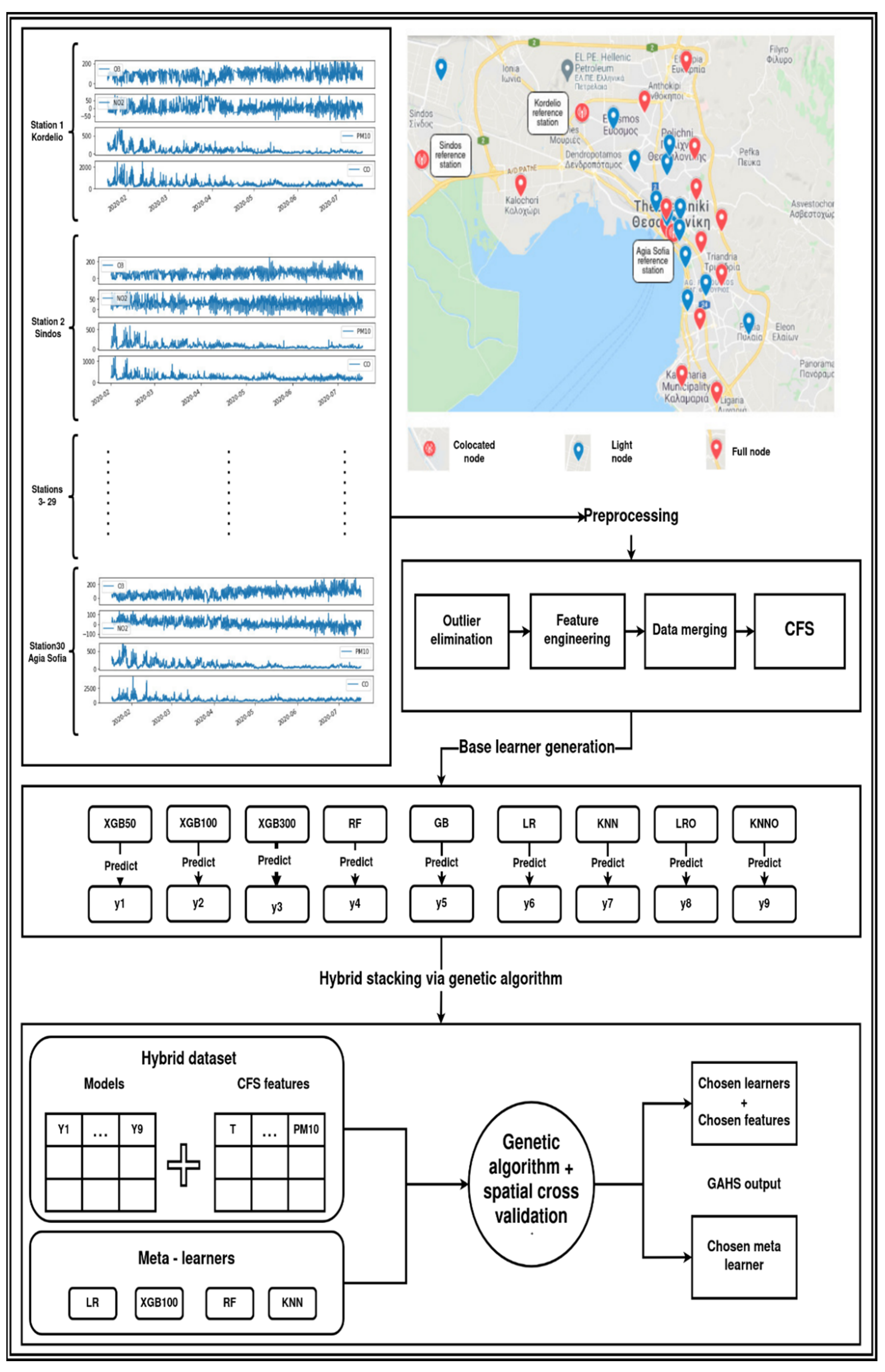
2.1. Experimental Design

The AQLCSN is operating as part of the KASTOM project [27]. Initially, 33 multi-sensor devices were installed to facilitate the AQLCSN, accompanied with three LoRaWAN transmitters to collect the data. All nodes can estimate coarse (PM10), fine (PM2.5) and ultra-fine (PM1) particulate matter concentration levels with the help of an optical particle counter sensor (Manufacturer: Plantower PMS5003). The devices are also complemented with meteorological sensors (ΒΜΕ280—Bosch Sensortech) for temperature (T), relative humidity (RH) and barometric pressure (P). In addition, twenty of them (the so-called full nodes), also include electrochemical gas sensors (Alphasense) to monitor concentration levels of carbon monoxide (CO), ground level ozone (O3) and nitrogen dioxide (NO2). PM10 reference concentration levels are estimated with the aid of an analyzer (Eberline FH 62 I-R, reference equivalence with European Standard EN 12341) that uses β-attenuation, while reference O3 concentration levels are measured with the aid of UV photometry according to European Standard EN 14625. The devices were strategically placed to cover most of the city with emphasis in the city center as depicted on the map in Figure 1.
Three of the devices are collocated with three of the reference stations (Sindos, Agia Sofia and Kordelio) operated by the Prefecture of Central Macedonia, to collect high quality ground truth readings and facilitate a supervised ML methodology to calculate calibration functions for each pollutant monitored via the AQLCSN. The data collection takes place every minute from nodes and the readings are aggregated by calculating the median value on an hourly basis. Missing values were minimally present in the minute resolution and were ignored during this stage. Additionally, missing values were present in the hourly resolution due to malfunctions of the sensors in need of repair. An imputation approach was investigated but the relevant periods were long, and imputation injected low quality data that in turn led to worse models therefore the missing periods were omitted for the hourly resolution too. The problem is designed as a regression modelling where the input X initially contains all measurements from the LCS and the output y corresponds to the pollutant, for which we calculate the calibration function, compared to the measured values produced by the reference instruments.

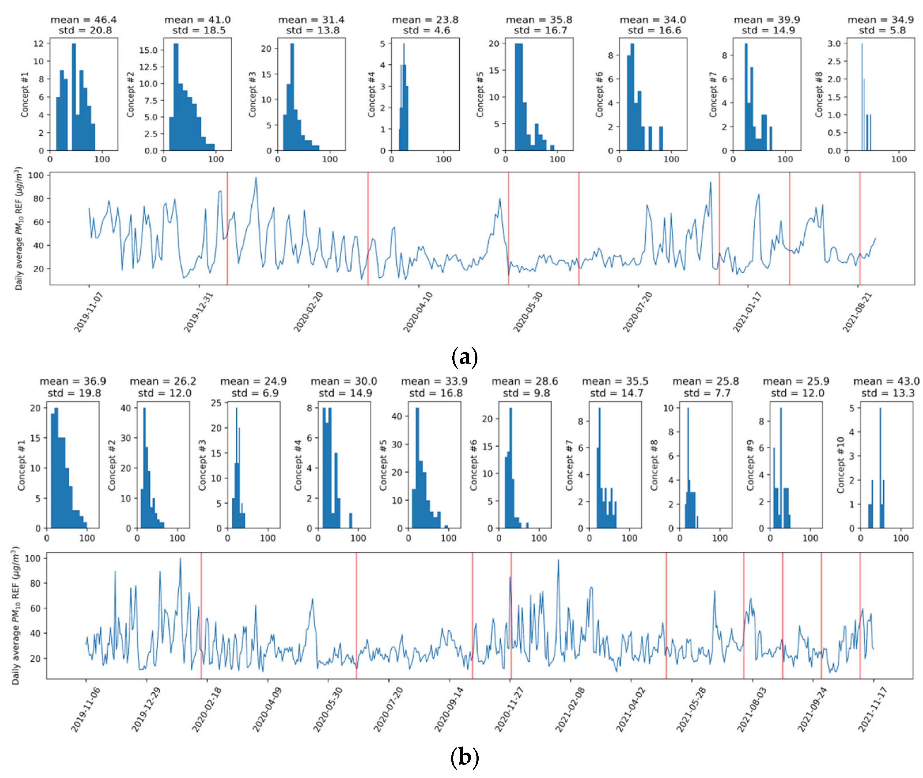
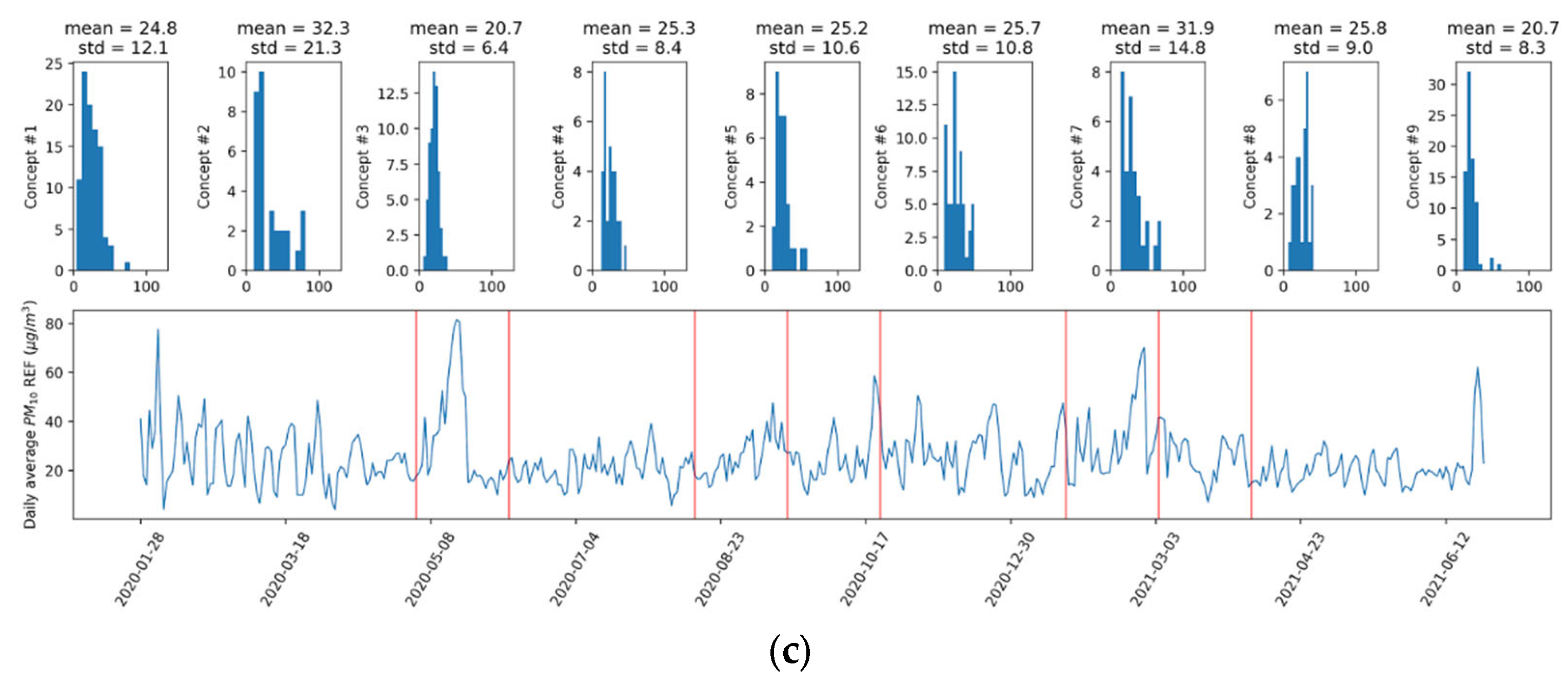
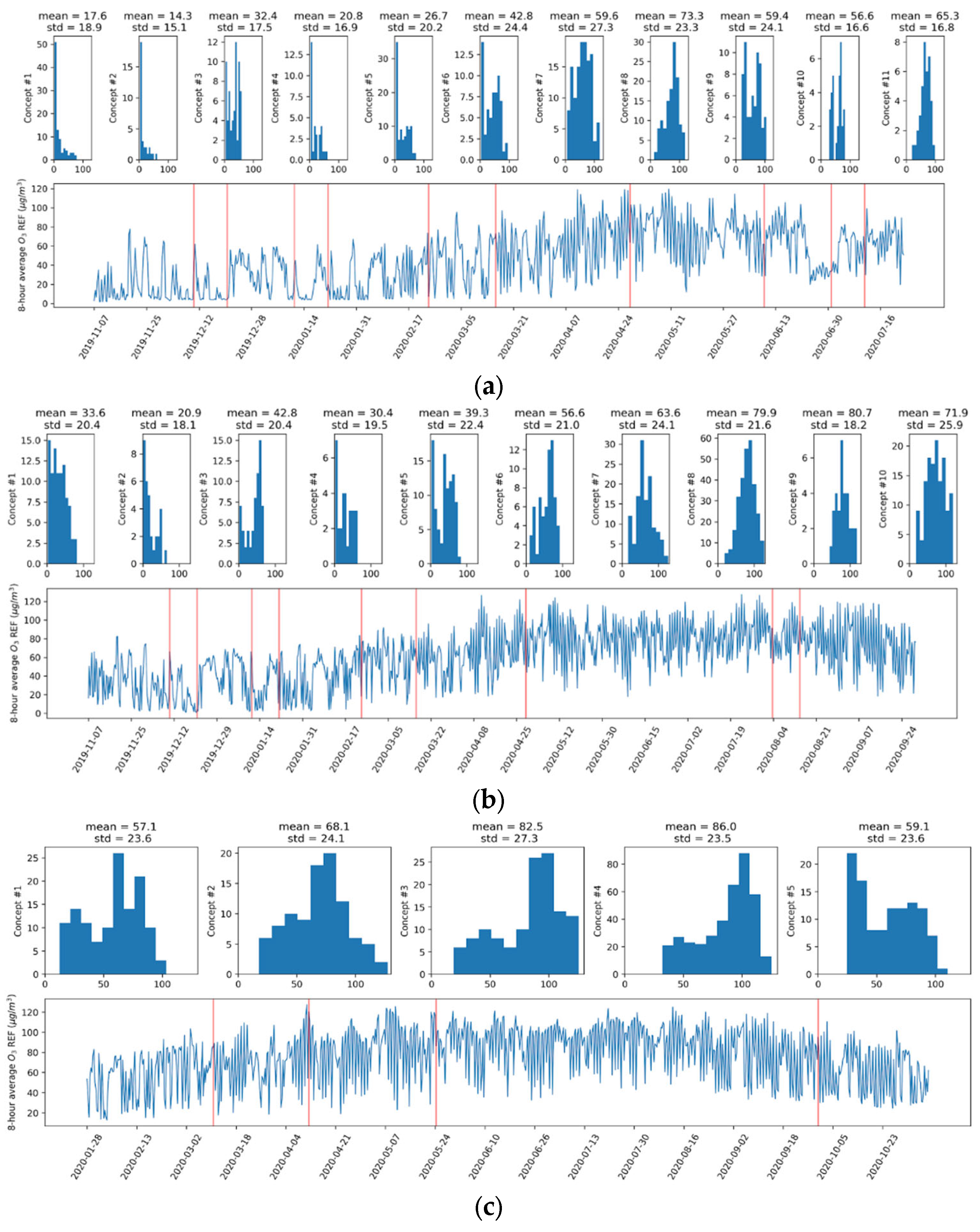
2.2. Concept Drift Definition and Detection

The formal way of defining a concept drift is by employing Bayes’ law. Given a stream of input-target pairs (X, y) the concept is defined as the joint probability distribution Pt(X, y) at time t and can be expressed as follows: Pt(X, y) = Pt(y, X) ∗ Pt(X) where Pt(y, X) is the posterior probability of the target y given input X and Pt(X) is the prior distribution of the input space [28]. A concept drift occurs when Pt+1(X, y)  Pt(X, y) and can be explained as the spatially or temporally related changes in the characteristics of features X, which affect the performance of a model that infers the target y, therefore leading to the need of its recalibration [29]. Such a drift can be further divided into three categories according to the factor of the above equation that shifts: (1) Pt+1(X)  Pt(X), called a virtual drift, because it does not cause performance degradation, and may be associated with seasonal changes of the features; (2) Pt+1(y, X)  Pt(y, X), called a real drift as it effectively alters the distribution between input-target pairs; and (3) both real and virtual drifts occurring at the same time. [30] provides a clear overview of the state-of-the-art approaches in the field and its implications in modeling.
To portray that indeed concept drift [31] occurs, we took advantage of the simple yet powerful adaptive windowing (ADWIN) algorithm [32]. ADWIN operates on an instance basis allowing for an incremental window to grow as long as there are no drifts detected. In the face of a drift, ADWIN removes the old concept instances and shrinks the window adapting to the new concept. In this study, the ADWIN algorithm is used to detect different concepts (altered distributions) for the reference time series of the two pollutants (PM10 and ozone). There is only one parameter, “delta”, which controls the sensitivity of classifying the result as a drift. The threshold value delta was set equal to 1 after manual investigation and visual inspection for meaningful concepts.

2.3. Spatial Online Learning

In the established online-incremental learning approach, training and inference are entangled procedures where the model produces an estimation at time t and then it is updated with single instances (Xn,t, yn,t) once the reference value is available where n represents the specific collocated pair in our setting. This approach was originally designed to forecast a single monitored time series one step ahead; however, in this study, the goal is spatial generalization nowcasting to multiple locations, thus the need of an extension is present for this problem. Relying on the idea of transfer calibration [8] and in order to train a spatially generalizable online-incremental ML regressor, we extend the idea of online learning to spatial online learning, under the assumption of identical replicable LCS devices, ensuring the transferability of learned patterns to different locations. In SOL, data are ingested by sequentially introducing a set of new entries collected from the collocated pairs at time t to a single online learner. The vector Z = [(X1,t, y1,t), (X2,t, y2,t), …, (Xn,t, yn,t)] defines a training instance of the spatial online regressor. Afterward, the learner can extrapolate at all the other locations Zother = [Xn+1,t, Xn+2,t, …, Xn+m,t] until new entries arrive. Here, Xn,j, j = 1, …, n is the vector of a number of n LCS measurements being collocated with reference instruments and yj, j = 1, …, n the ground truth value of the target parameter for the calibration function and (mn) is the number of the uncollocated sensors. In the ideal case where reference entries arrive hourly, the SOL framework allows the learner to be updated at time t and also infer at time t to all other locations, thus obtaining the most accurate estimations. Following this approach, the slow adaptation of online learners to new concepts [33] is ameliorated as they are effectively transformed to batch learners but with each batch containing timely and spatially relevant data for the current concept. This way the learner “sees” information about the state of the whole AQLCSN compared to the reference network. Furthermore, the SOL regressor is offered a wider variety of environmental conditions extending the validity domain of inference.
As the database expands, the batch models are retrained in an incremental way adding the latest data for training. On the one hand, SOL training can follow the example of “traditional” incremental learning and lose access to previous instances. On the other hand, we observed that retraining online models the same way batch models are trained (concatenating the time series without shuffling) and then applying the SOL framework for the evaluation month, yielded more accurate results than the alternative. The intuition is that the mixing adds noise to the temporal patterns that the models try to extract; however, it also adds value by ameliorating the concept drifts. We believe that retraining on the original time series, up to the point of operational reinitialization of the calibration, helps the online models learn the temporal sequencing; while updating with the SOL framework, mostly benefits the models to adapt to concept drifts during operational calibration.

2.4. Preprocessing

Initially, the readings from the LCS and from the reference instruments were synchronized. Afterwards, outliers were identified as the values that fall outside of the range [median −3*std, median +3*std] with the statistics being calculated over the whole period of measurements and were eliminated by replacing them with NaN placeholders. This concludes the data cleaning, and the analysis continues with feature engineering comprising three main approaches: (1) variable combination; (2) rolling statistics; and (3) lags. Variable combination aims at modeling some of the interactions between the measured time series and are represented as fractions. Given an instance, Xt (PM1t, PM2,5t, PM10t, Tt, RHt, Pt, O3t, NO2t, COt, RHt/PM1t, PM10t/RHt, NO2t/O3t, NO2t/Tt, O3t/Tt, Tt/Pt, Tt/RHt, Pt/RHt) at time t, we compute descriptive statistics and the difference between the minimum and the maximum of the last 24 and 48 h on a rolling basis to inform the input vector and, consequently, the learners about the long-term statistical behavior of the AQLCSN and provide the models with smoother, less noisy versions of the initial features. Furthermore, we complement the instance with the last 12 raw measurements of each variable to inform the models about the short-term behavior of the AQLCSN. After the engineering, the following features are extracted from PM1: PM1t, PM1t−1, PM1t−2, , PM1t−12, mean(PM1, 48), mean(PM1, 24), std(PM1, 48), std(PM1, 24), min(PM1, 48), min(PM1, 24), max(PM1, 48), max(PM1, 24), median(PM1, 48), median(PM1, 24), min_max_diff(PM1, 48), min_max_diff(PM1, 24). All the above actions are performed for each station separately to avoid leaking information from one station to the other. Finally, the data are merged row-wise into one single dataset. The overproduction of engineered features introduces multicollinearity to the data, therefore a feature selection process should follow to identify the best uncorrelated predictors. In this work, we consider the fast and accurate correlation-based feature selection (CFS) method [34] as implemented in the WEKA ML package [35].

2.5. Base Learners Generation

A wide range of linear, tree-based ensembles and distance-based algorithms are chosen to implement the generation of base learners. We employ three different ensembling strategies, namely, random forest (RF), gradient boosting (GB) and extreme gradient boosting (XGboost) for their inherent non-linear functionality. The RF is an ensemble learning algorithm that employs the bootstrap sampling method, creating a decision tree per sample (therefore, all trees are created independently to each other), and combining their predictions in an averaging approach towards the final model result [36]. GB is also an ensemble learning algorithm based on decision trees, where one tree is created after the other, correcting the weaknesses of the previously developed trees (boosting performance), and the ensemble is also created gradually and in parallel with trees [37]. Xgboost applies the same boosting principle with improved (more regularized) model formalization to control over-fitting, usually leading to better results [38].
The RF, GB, XGB100 contain 100 regression trees; however, the Xgboost algorithm is considered state-of-the-art for tabular data, thus we exploit this by producing two more models with 50 and 300 trees. The focus was drawn away from hyperparameter tuning of these algorithms contrary to the expectation, considering that the purpose of these models is not the selection of the best model, rather it is to provide information to another model, the meta-learner (Section 2.6), and are better considered as feature extractors. Furthermore, two versions of the multiple linear regression (LR) are incorporated. The former is a standard batch LR as implemented in “scikit-learn” python package and the latter is the online–incremental version namely multiple linear regression online (LRO), optimized with the Rmprop optimization algorithm and can be found in the “river” [39] python package. The k-nearest neighbors (KNN) pattern classification algorithm [40] operates on a high dimensional space and calculates the distance between an instance and the k-nearest neighbors. When the optimization objective is reached, the produced model can infer a new estimation based on the similarity of the new instance with the k-nearest neighbors by averaging the known values of the training data. Both batch and online versions namely k-nearest neighbors online (KNNO) are incorporated again from the same python packages. LRO and KNNO are trained within the framework of SOL (Section 2.3).

2.6. Hybrid Stacking Optimization via a Genetic Algorithm, the GAHS Framework

Stacking has been successful in combining well performing models produced by different algorithms [41], whereas bagging and boosting combine the outputs from the same (high variance) models with emphasis on the reduction of variance. The motivation behind the decision to include stacking lies on the models’ agnostic architecture, which offers the potential to combine different modeling approaches. The GAHS framework is structured with spatial generalization, ensemble adaptation [42] and modularity in mind, therefore, the spatial cross validation is integrated, and the components (features selection, base and meta learners) can easily be replaced. With the aim of producing a target (pollutant) agnostic framework too, we alleviate the need for model selection, which is dependent on the target, by assigning this task to the GA. Therefore, the same framework works for both pollutant species addressed in this paper (PM10 and O3) out of the box. In our approach, we choose to extend stacking in two ways: (1) by concatenating the base-models predictions along with the CFS selected features and introducing the combination to the meta-learners as a hybrid input space; and (2) by optimizing the best combination of base-learners, CFS features and meta-learners simultaneously via a modified version of the GA. Analytically, the GA operates on a boolean vector where the first N values correspond to the CFS features, the next M values represent the model predictions (whether to be included) and the last four values of the vector represent the meta-learners. Because only one meta-learner can be trained at each generation, in the last four values only one can be true. To navigate this issue, if two or more true values appear, then we artificially assign a negative score (−9999) to this combination at the evaluation stage when optimizing for the coefficient of determination R2 and a highly positive score (+9999) when the optimization objective is the mean squared error, thus it naturally converges to solutions with one meta-learner. In order to train base learners that possess the ability to generalize at different spatial locations, spatial k-fold cross-validation [43] in the form of “leave one out” is performed to produce the predictions that will later serve as input to the meta-learner training phase. To elaborate, the models are trained on two reference stations and the third is used for validation in a cyclically repeated way. The framework outputs the learned models and the optimized boolean vector that describes which features, base-learners and meta-learner are included.

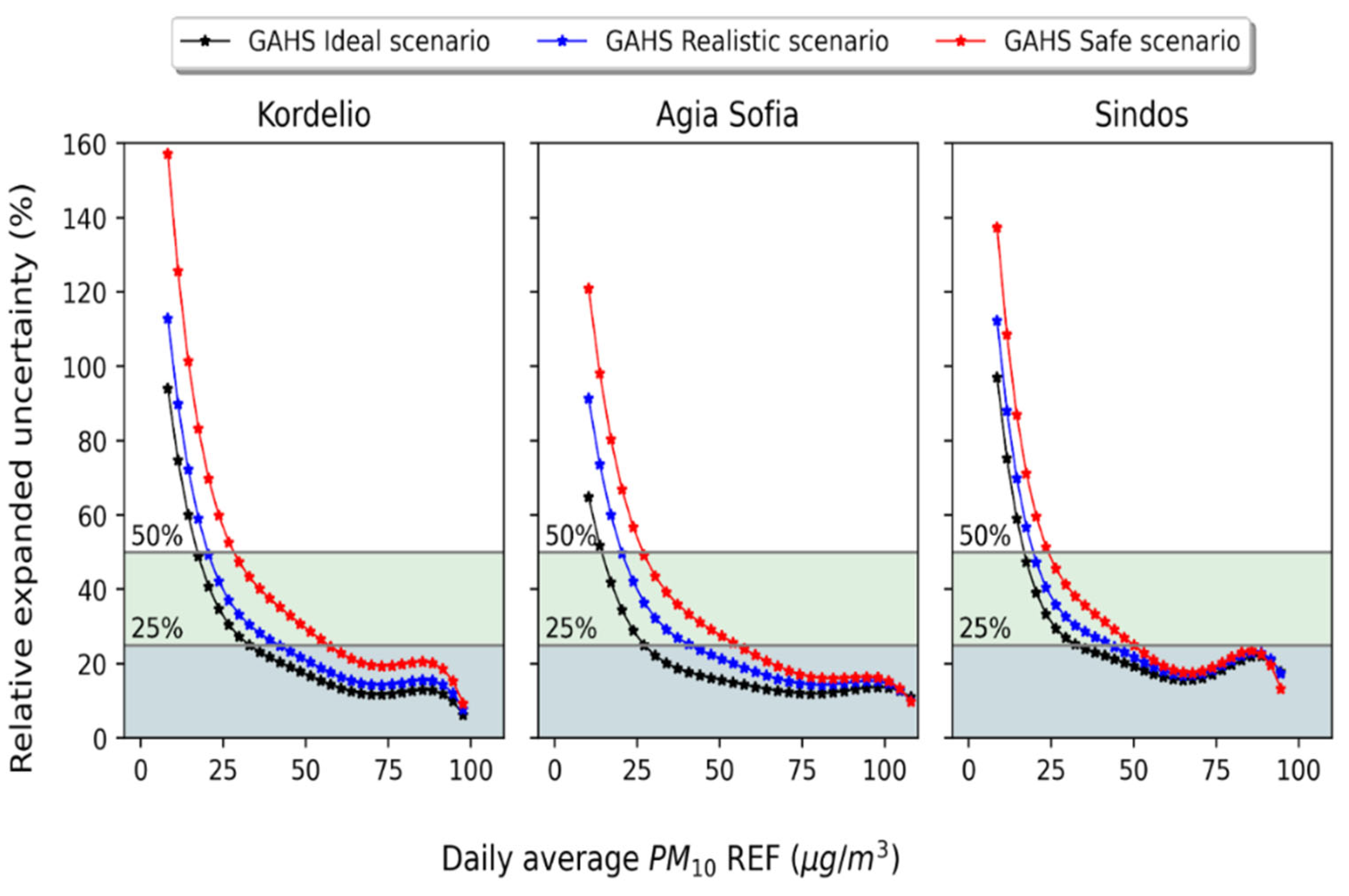
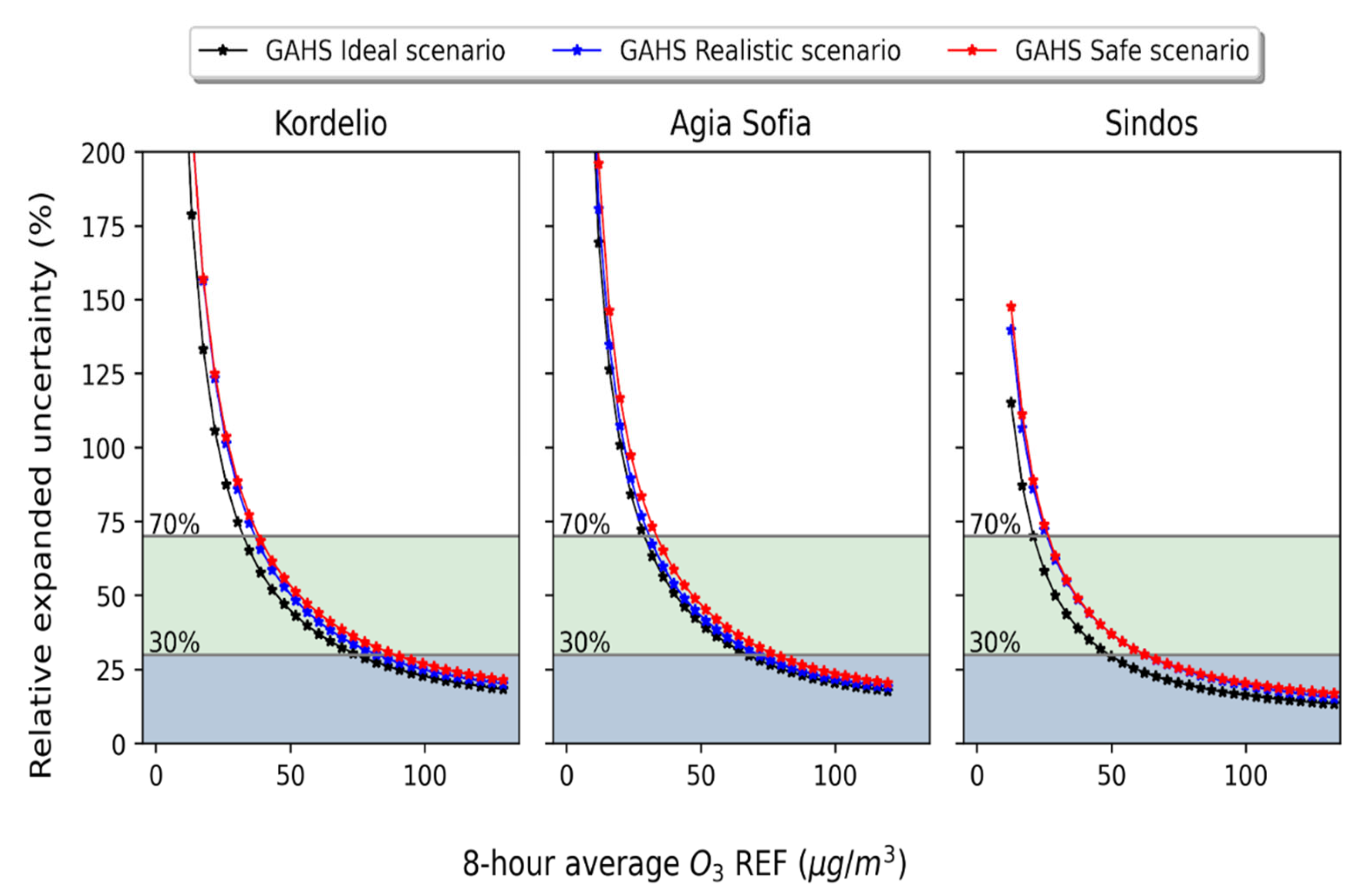
2.7. Evaluation of Operational Scenarios

Evaluation starts as soon as two months of hourly measurements have been collected from the three collocated sensor-reference pairs: first month measurements serve as training and validation data, while the remaining data are being used to test the calibration in a forward manner. This forward CV process repeats incrementally, and the evaluation always refers to the last month. The batch learners train on the concatenated dataset (without shuffling) and provide estimations for the whole test month and are retrained only when the next month’s data are made available. Online learners learn by single instances and therefore require the previous hour’s reference measurements to be available before the next hour’s estimation is produced (ideal scenario). This is often infeasible because the reference data are not available in real time; however, one can overcome this issue in operational mode by delaying the learning-updating phase for some amount of time, sacrificing some accuracy on the way. Toward this end, apart from the ideal scenario, two more scenarios are implemented where the learning process is delayed by five hours (realistic scenario) and by twelve hours (safe scenario). Reference measurements are automatically obtained via the EEA API response on an hourly schedule and the response is examined for new entries compared with the previous hour’s response. For the case of Thessaloniki, there are new entries every three to seven hours and not always from the same station, thus we average and use the five-hour delay as the closest to real operational delays.
Apart from the regression statistical indices that are presented in Table 1, we also incorporate the Pearson correlation coefficient and the relative expanded uncertainty as defined by the Dir. 2008 EC [44] to assess the quality of the calibration. The REU has been calculated on the basis of the methodology described by [45] and making use of Equations (1) and (2).
U r y i   = 2 R S S n 2 u 2 x i + b 0 + b 1 1 x i 2 1 2 y i ,
R S S = i y i b 0 b 1 x i 2 ,
Here Ui(yi), is the relative expanded uncertainty, u2(xi) is the random uncertainty of the standard method here set equal to 0.67 for PM10 and 0.0 for O3, RSS represents the sum of (relative) residuals, xi is the average result of the reference method over period I, yi is the average result of the model over period I, while b0 and b1, are the coefficients of the regression y = b1 x + b0. For PM10 measurements to be considered as indicative or fixed, REU should be below 50% and 25%, respectively. The criterion is implemented for daily averages. Ozone LCS measurements should be below 70% and 30% implemented for 8 h averages.

3. Results

3.1. Drift Detection

To quantify the concept drift, the reference pollutant measurements were aggregated to meaningful 24 h averages for particles (PM10) and 8 h averages for ozone, and the ADWIN drift detection algorithm was applied. The results are depicted as red vertical in Figure 2 and Figure 3. Furthermore, a set of histograms corresponding to the detected intervals are depicted in a sequential way. The mean and standard deviation are calculated to quantify the changes. Most of the segments are meaningful in detecting changes in the statistics; however, there are cases where it is visibly not a good threshold. Regardless of ADWINs accuracy, the concept drift can also be observed in the distributional changes over time. Each distribution represents the detected concept and their sequence represents the evolution of the concepts in time. An interesting instance is the PM10 time series in Kordelio. The expected distribution resembles concept #1 for winter. Moving forward in time, the distribution shrinks (concept #3 and #4), which is characteristic for the spring–summer periods in Thessaloniki mostly due to reduced domestic heating. In concept #5, that lasts for the whole winter period of 2020–2021, the distribution returns to its original form with similar statistics. Evidently this is caused by seasonality and is related to meteorology; however, from the concept point of view this can be translated to a reoccurring concept drift. As is also indicated from the regression metrics in Section 3.3, the winter concept has clear patterns to model and the metrics agree; however, during the summer the measurements are far noisier with less variance and the models struggle. Ozone on the other hand, shows stable variance except for the winter months where the pollution levels are low, and the noisy pattern problem arises here too. For this case, mostly the mean shifts are observed, which is again related to the meteorology.

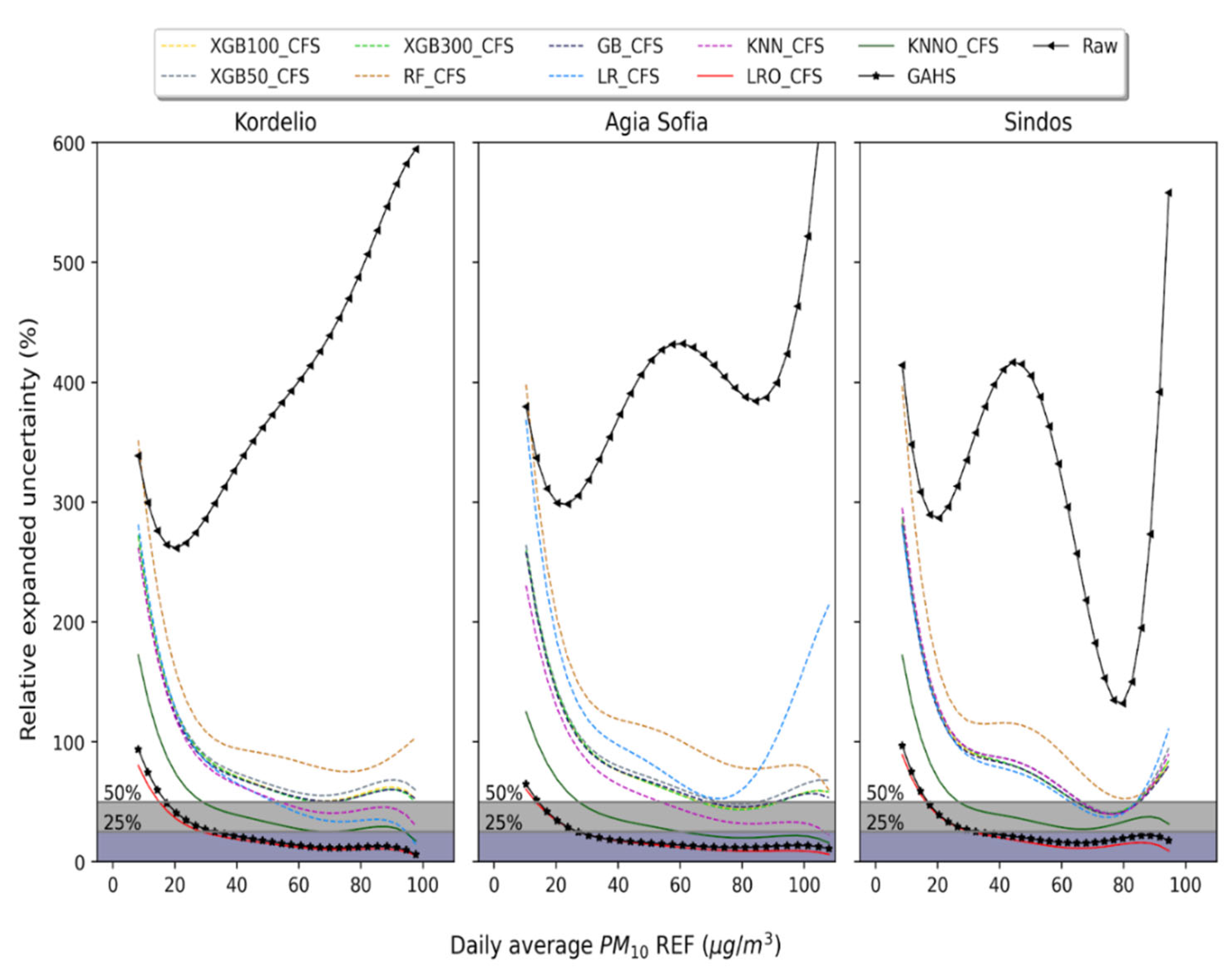
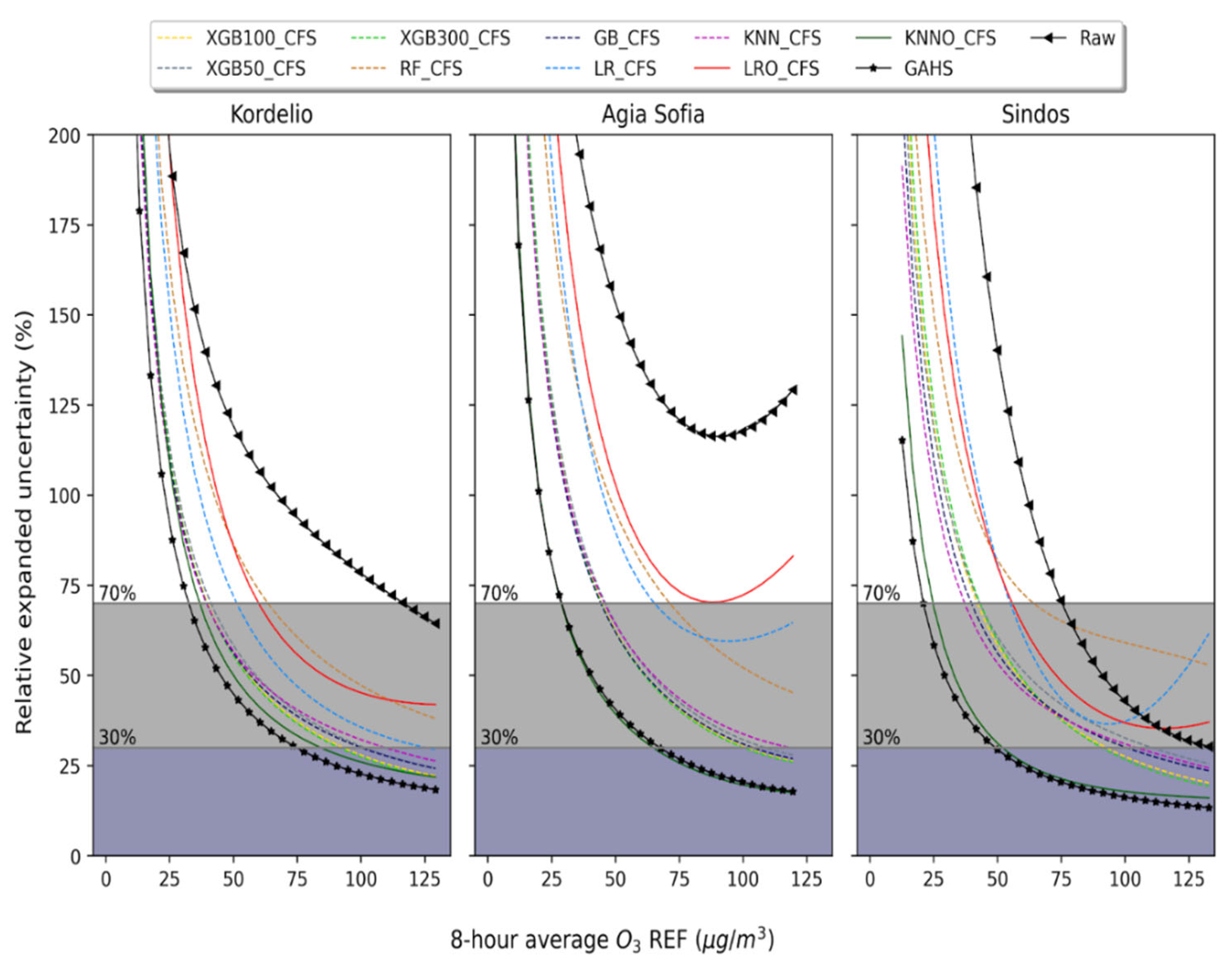
3.2. Relative Expanded Uncertainty

For the ideal case (reference measurements available instantly), Figure 4 and Figure 5 demonstrate the REU over all measured values. First, it is clear that the raw measurements fail to provide data within the targeted REU levels, for both pollutants, and all locations. Furthermore, it is evident that the SOL models behave much better and can remain within the levels when the batch versions in some cases fail to reduce the REU enough to comply with the directive. Regarding PM10 the performance of our approach is almost identical to the LRO but for ozone surpasses all the base learners. This indicates that when appropriate the meta learner will discover a better performing combination than each individual regressor but will choose (highest weight) to use the best base regressor when the former is infeasible. A notable difference between the improvement achieved for PM10 and O3 is that for the former the concentration range within which the REU decreases and therefore improves is much higher, while in both cases low pollutant concentrations are always characterized by higher REU.
As was mentioned, the ideal scenario is difficult to be implemented, thus the effect that the delay produces to the calibration functions REU is presented in Figure 6 and Figure 7. All the subgraphs demonstrate that uncertainty increases with delay, but the performance remains under the desired level for the most part, even for the safe scenario.

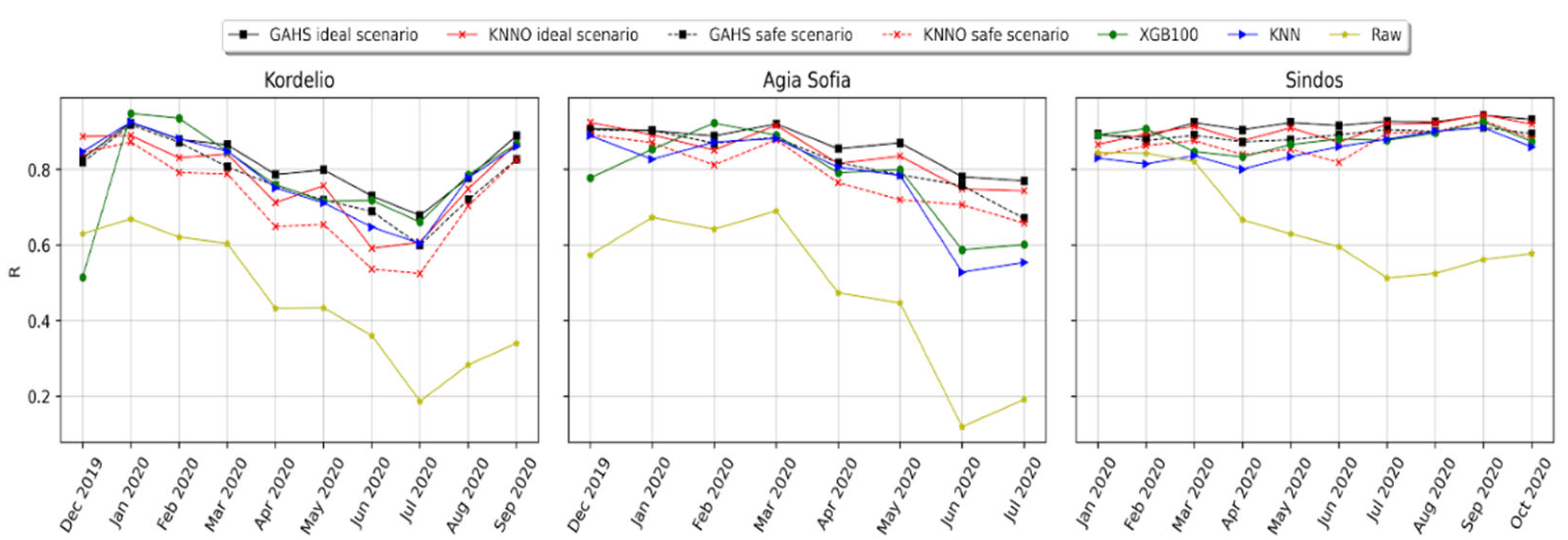
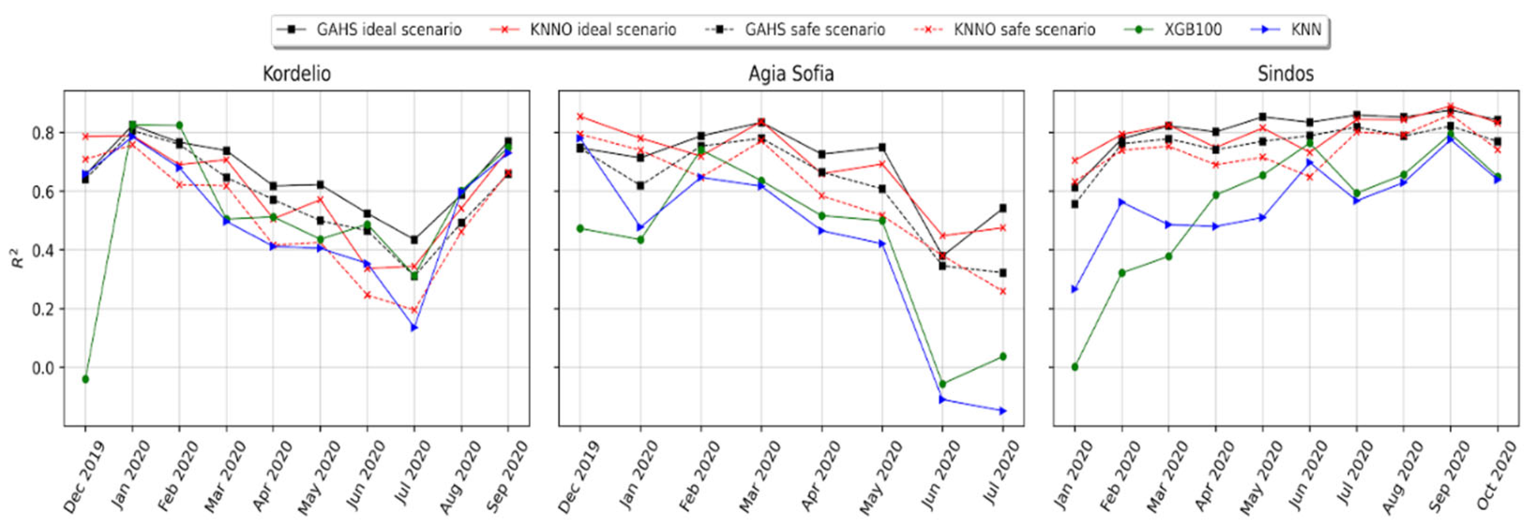
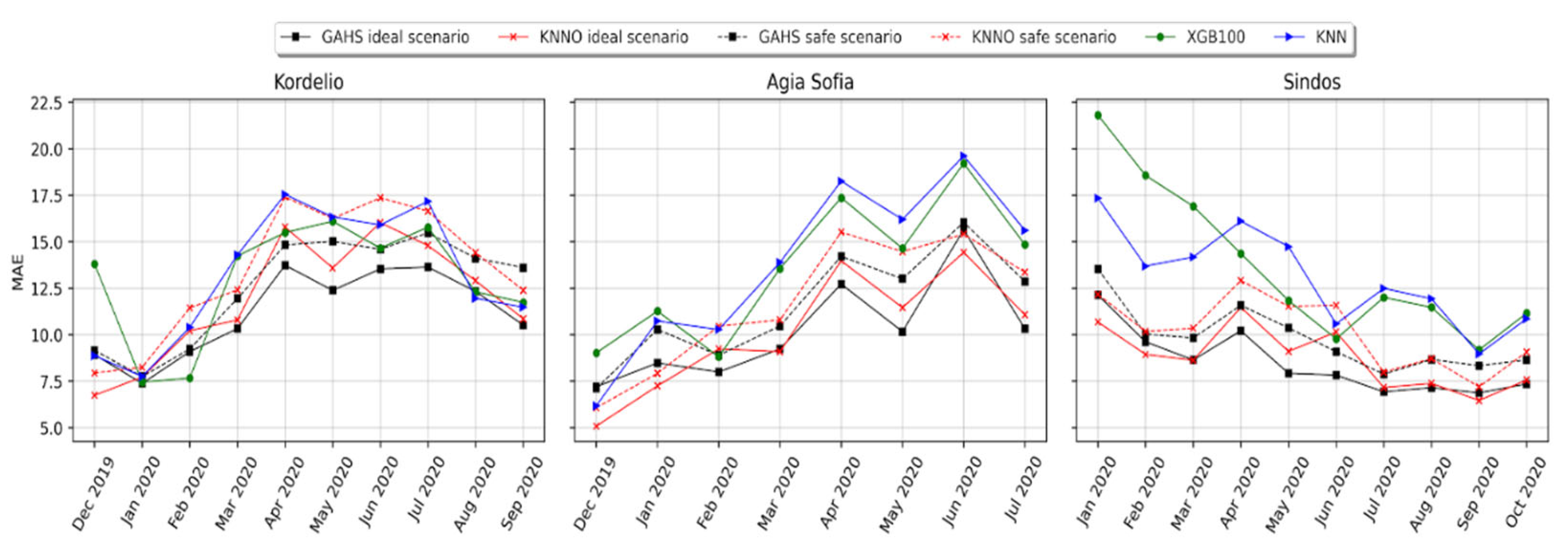
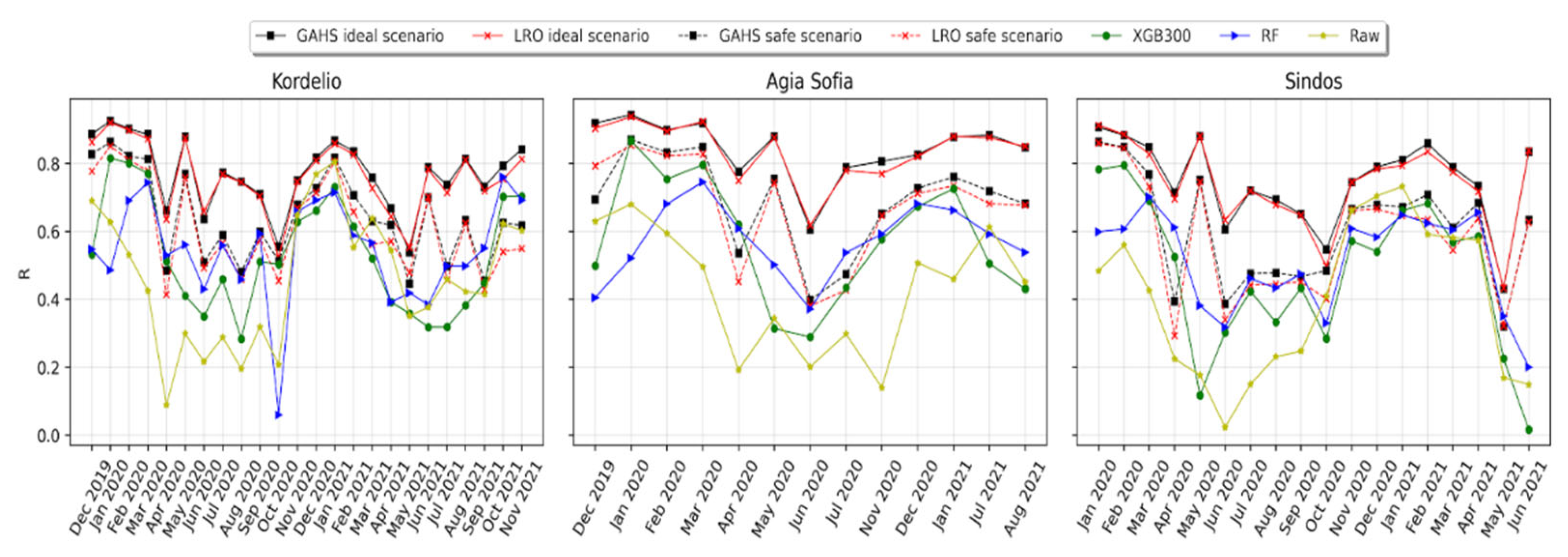
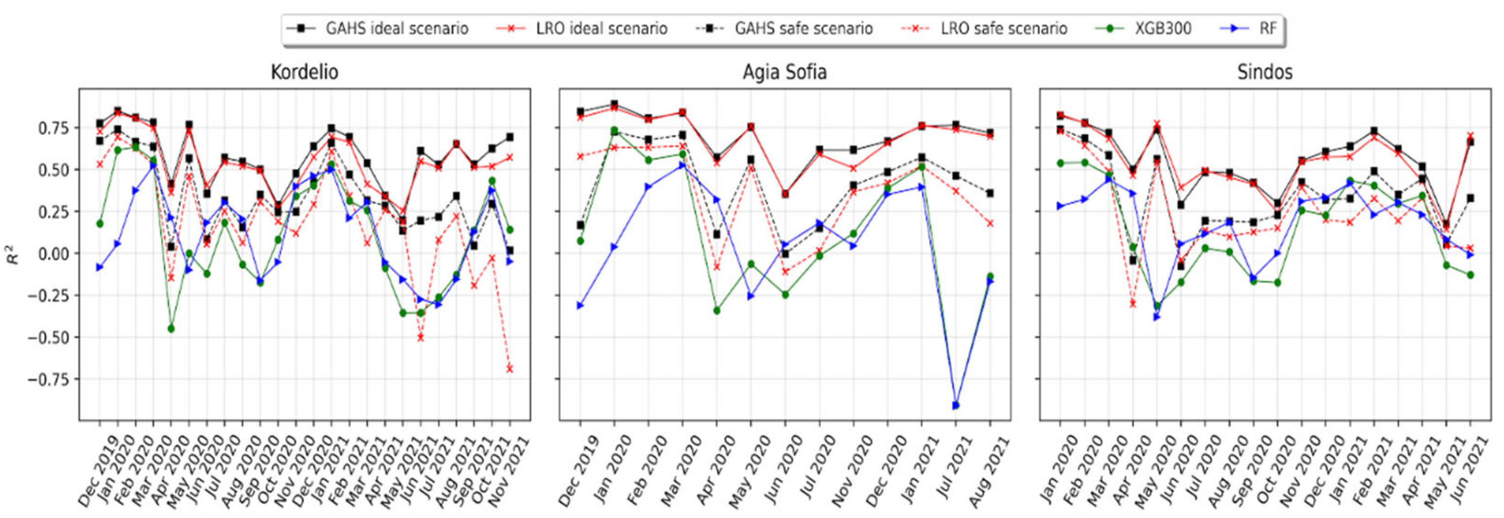
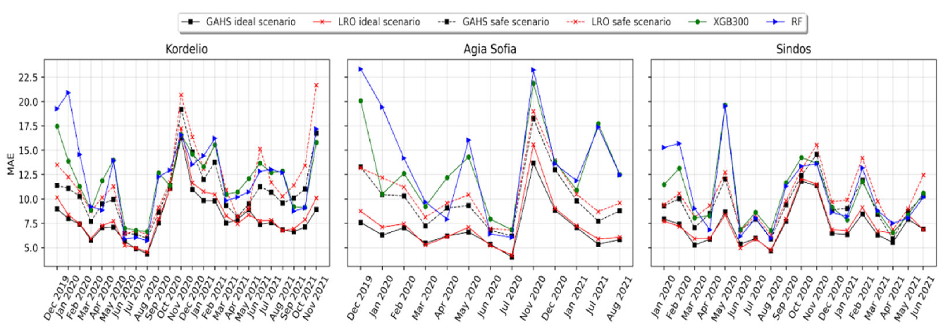
3.3. Forward Evaluation of the Calibration Framework

Ozone calibration is evaluated for a duration of 10, 8, 10 months in Kordelio, Agia Sofia, and Sindos, respectively, in Figure 8, Figure 9 and Figure 10. After this period the sensors started producing extremely negative values yet still correlated with the reference. These values, however, were omitted mainly for two reasons. Firstly, these abrupt shifts in the mean of the sensor response break the continuity of the time series rapidly making all the previous training data obsolete even if correlations still exist. Secondly, electrochemical sensors last for at least one year; however, operation in high humidity and high heat conditions that characterize the summer period in Thessaloniki, significantly reduces their lifespan [46]. Examining the performance forward in time offers the opportunity to observe how the calibration responds to drifts. Specifically, the Pearson correlation R between the reference and the raw measurements drops with time thus altering the relationship between the two. The coefficient of determination is the hardest metric to stabilize above a certain level for long periods because as R drifts, past information gradually becomes obsolete, which is highlighted in the ability of the models to accurately estimate. The proposed methodology manages to keep the ozone LCS operational and highly accurate for 8 to 10 months. During the first two months of deployment, the SOL approach dominates because it requires less data to converge being simpler, whereas from the third month onwards the GAHS approach outperforms both the SOL and the batch on almost all months. It is worth noting that while the sensors drift, which is depicted by the reducing correlations, both GAHS and SOL manage to adapt and maintain high accuracy much better than their batch counterparts.
Particle counters demonstrate a more diverse functioning in Figure 11, Figure 12 and Figure 13 and are evaluated for 24, 13, and 18 months in Kordelio, Agia Sofia, and Sindos, respectively, giving the opportunity to study the long-term behavior of the sensors and their calibration. Focusing on R between the raw sensor data against the reference data, we observe that during the winter the relationship strengthens with higher correlation values and during summer periods the relationship is weakened. It also exhibits oscillatory behavior between months when a constant value was expected, which demonstrates the seasonal variations’ role in the ability of the LCS to correctly capture particle-related AQ. This indicates the presence of abrupt as well as recurring drifts leading to reduced performance. It is evident that the specific configuration of the sensors and, subsequently, the calibration procedure have a hard time modeling PM10 during the summer period when the domestic heating emissions are low and dust contribution becomes more relevant. While we recognize that PMS5003 cannot accurately distinguish PM10 from PM2.5 [47], they can be calibrated to yield indicative measurements in terms of REU, especially during the presence of high pollutant concentrations from domestic heating (winter). In the ideal case, the GAHS and the SOL perform almost identically, far surpassing the batch algorithms that they are compared with. The relevance of delaying is much more evident in regression metrics than it is in the REU. Regarding the safe scenario, the coefficient of determination for Kordelio has some notable instances of GAHS outperforming the SOL framework. For the whole period up to a point LRO closely follows the GAHS performance. From June to September the LRO model starts deteriorating but the GAHS framework continues to operate at some accuracy. Another notable instance can be observed at Agia Sofia R2. The last two months of the series are collected six months (due to repairments) later than the previous data. Nevertheless, we included these two months to simulate the adaptation of a newly installed LCS. Demonstrably, GAHS and LRO rapidly adapt to the new concept with decent accuracy, but the batch learners fail with negative scores. In the last three months the batch models start to outperform the LRO and the GAHS framework updates the combination it uses to rely more on batch models as they become more appropriate. Finally, focusing on Sindos and comparing the GAHS and LRO for the last month, we observe that both approaches produce the same correlation around 0.6; however, examining the R2 plots, the GAHS value is around 0.3, while the LRO value is zero.

3.4. Comparison of the GAHS, SOL and Batch Algorithms

Aiming to determine the influence of CFS features and base learner estimations to the meta-learner, GAHS runs monthly with frequent updates for the SOL leaners, and the chosen feature-learner sets are collected. The expectation was that the base learner predictions will be chosen more often due to higher correlation with the target than the already processed features and is confirmed because O3 depends mostly on KNNO while PM10 depends more on LRO as they appear to contribute to all the evaluation months. This confirms that selecting the best algorithm is dependent upon the target among others. However, it is irrelevant to the GAHS framework as it automatically selects the best modeling combination of features and algorithms making it agnostic to the target. Out of the batch algorithms, the KNN is chosen more often followed by the RF, GB and then XGboost. The differences between them, however, are marginal. The highest contributor feature for ozone is the RH range of the last 48 h (rolling_min_max_diff_humidity_48) followed by the same range of the fraction temperature/pressure (rolling_min_max_diff_T/P_48). This indicates that: (1) the long-term meteorological conditions play an important role in modeling the calibration functions; and (2) the base learners struggle to extract patterns in the first stage of stacking and thus reintroducing them to the next processing level adds value to the meta-learner. Generally, meteorological variables and their combinations with pollutants (e.g., rolling_min_RH/PM1_48) dominate the feature space. As was mentioned, for PM10, modeling gaseous pollutants were not included. In this case, most of the features appear only once. Interestingly enough, the minimum value of RH/PM1 fraction is the best feature for particles too (rolling_min_RH/PM1_24) but in the 24 h, shorter time interval. Moreover, PM10/RH first 4 lags have a high contribution as well as indicating that a nonlinear relationship between the two and the target is present, manifesting as linearity between the target and the fraction. Consistently, LR is chosen as the meta-learner, which is convenient because it is also the fastest algorithm. In Figure 14 for particles and Figure 15 for ozone, the calibrated response from several different locations is presented concerning one of the last months of evaluation. Respectively, for Figure 16 and Figure 17 the calibrated response of a collocated node against the reference is depicted on the right panels, while the linearity between them is depicted on the left panels. A good agreement is observed for both pollutants. All the LCS time series follow the pattern of the collocated series. Deviations can be located at the peaks for PM10 where different LCS peak at different times. Deviations for ozone are more visible in the valleys where LCS take much more time to reach the low-end value compared to others. This suggests that responding to the raw LCS readings the learners can adjust their estimations accordingly. For a detailed visual inspection of the calibrated output against the reference measurements as well as the feature-base learner bar plots the reader can refer to the Supplementary Materials Figures S1 and S3–S8, respectively.

4. Discussion

4.1. The Relocation Problem

As the blind and the chain calibration methods (Section 2) are not capable of properly representing the spatial nature of the LCS measurements, a transfer calibration, which is the category that the approach of this study falls into is applied. This calibration method learns the function on a collocated (master) node and then the function is applied to another non-master node according to proximity or similarity. The presented method differs from the usual transfer calibration in considering the calibration of the whole network with a single function in the SOL framework. So, relocation is addressed by fixing the LCS to their deployment location under the assumption that the devices provide similar measurements under the same conditions. We propose to collocate a copy of the LCS with all the available reference stations and place all other LCS to their assigned positions. Sampling the region with two overlapping networks where the LCSN is calibrated to match the reference networks, spatially generalizable calibration function can be achieved by optimizing the base learners with spatial k-fold cross validation with k being the number of available reference locations.

4.2. On-Site Continuous Evaluation

For the calibration of the LCS network several studies have concluded [48,49,50] that a machine learned calibration function should be included in the deployment. A necessary step is therefore the evaluation of the ML models on site, for which the usual way applied is with train-test splits and k-fold CV approaches [51]. The former offer only a glance on the specific data and do not confirm the continual generalization of the models. On the contrary, a comprehensive discussion of CV methods for LCS calibration [50] concludes that spatial CV in the form of “leave one out” or “leave all but one out” is the most relevant method. This statement finds us in agreement considering that the goal is to produce spatially generalizable regressors for transfer calibration. Yet there is a caveat that requires attention, to avoid information leakage: in the AQ monitoring setting, for example, random shuffling CV allows future information to penetrate the training set leading to overconfident estimates in the validation set but to reduced performance in deployment. For this reason, what we apply instead is a combination of spatial and forward CV to obtain a realistic view of the on-site calibration performance. Compared to our previous study [52], where we used time-block CV without shuffling and managed to achieve improved uncertainty with batch algorithms, this study indicates that in the spatial–forward CV scheme they would probably perform worse and a SOL or a GAHS approach should be considered.
De Vito et. al. [53] highlight that the evaluation should be subject to robustness and identify the important role that drifts play to performance degradation. They introduce a drift monitoring quantitative framework based on the comparison of probability distributions dissimilarity of relevant pollutants during the calibration and deployment periods. Laref et. al. [54] on the other hand approach the drift correction of Alphasense NO2 LCS by splitting the calibration in meteorological and time components. The authors use the multiple linear regression model to correct for meteorological effects, then assume that the degradation through time is uniform and correct for time drifts by optimizing the parameters of an exponentially decaying model with particle swarm optimization. We also argue through the analysis of the study that one important aspect that affects the calibration of such a network is the drifting behavior of the LCS and the concept drift of reference measurements for both pollutants studied (Figure 2 and Figure 3). Based on [53] and the evaluation analysis of this study we suggest that during deployment the effect of these drifts, as well as the validity domain of the calibration functions, should be monitored and action for adaptation should be taken when necessary.

4.3. Limitations of the Study

The limitations of the study can be summarized as follows: PMS5003 optical particle counters cannot distinguish with the desired accuracy the particle sizes and especially struggle to infer PM10 concentrations when the PM2.5/PM10 fraction is small [47]. A more suitable PM10 LCS should be considered to improve the results. Access to high quality measurements is restricted (only three reference stations available) and thus a wider range (more collocated pairs) study will provide a more challenging and robust evaluation of the methods herein. In addition, a more robust online approach should be considered instead of the offline GA optimization algorithm [55], which retains the same features and models during the whole monthly testing phase but rather adapts to changes as soon as possible. Furthermore, more than one feature selection methods can be used in tandem to produce a diverse set of representations from the initial dataset and enrich the base-models space during the stacking stage. Of course, a general limitation is the disruption of continuous monitoring by glitches of the transmitters, power fluctuations, maintenance etc. and must be kept to a minimum to achieve consistent and reliable on-site calibration. Finally, long delays (>12 h) without new entries can reduce the accuracy of the calibration and thus real time access to reference data can greatly extend the ability of LCS to monitor AQ.

5. Conclusions

Our study highlighted that sensor drifts as well as seasonal variations and pollution episodes can be examined as concept drifts when calibrating AQ LCS under operational conditions. The main goal of the study was to introduce the SOL framework and compare it with batch learning algorithms. Moreover, the GAHS framework was proposed to combine batch and SOL ML algorithms (or any other kind of modeling algorithm as it is model agnostic) and address the stability-plasticity dilemma. Initially, the study focused on calibrating an AQLCSN against a reference network with a generalized online learner that observes the states of the two networks and updates the models as soon as high-quality measurements are rendered available. Later, a combination of spatial and forward evaluation frameworks was presented with monthly resolution. Results suggest that it is possible to arrive at improved LCS performance and to therefore improve the network’s capability to reflect actual air pollution levels as reported by ground truth observations in the studied area. Finally, it is highlighted that a continuous monitoring system should be considered to observe the calibration performance.

Supplementary Materials

The following supporting information can be downloaded at: https://www.mdpi.com/article/10.3390/atmos13030416/s1. Figure S1: Chosen features and models by the GA stacking. (a) corresponds to PM10 and (b) to O3. Figure S2: The calibrated output of the GA-stacking framework of 5 novel to the models nodes are presented for PM10 (a) and O3 pollutants (b). Figure S3: The calibrated output against reference readings for visual validation is presented in the right subfigure and the linearity is presented in the left. The results refer to the PM10 levels for the KORDELIO collocated node-reference pair for the ideal scenario. Figure S4: The calibrated output against reference readings for visual validation is presented in the right subfigure and the linearity is presented in the left. The results refer to the PM10 levels for the AGIA SOFIA collocated node-reference pair for the ideal scenario. Figure S5: The calibrated output against reference readings for visual validation is presented in the right subfigure and the linearity is presented in the left. The results refer to the PM10 levels for the SINDOS collocated node-reference pair for the ideal scenario. Figure S6: The calibrated output against reference readings for visual validation is presented in the right subfigure and the linearity is presented in the left. The results refer to the O3 levels for the KORDELIO collocated node-reference pair for the ideal scenario. Figure S7: The calibrated output against reference readings for visual validation is presented in the right subfigure and the linearity is presented in the left. The results refer to the O3 levels for the AGIA SOFIA collocated node-reference pair for the ideal scenario. Figure S8: The calibrated output against reference readings for visual validation is presented in the right subfigure and the linearity is presented in the left. The results refer to the O3 levels for the SINDOS collocated node-reference pair for the ideal scenario.

Author Contributions

Conceptualization, E.B., T.K. and K.K.; methodology, E.B.; software, E.B.; validation, E.B. and K.K.; resources, K.K.; data curation, E.B. and T.K.; writing—original draft preparation, E.B.; writing—review and editing, E.B., K.K. and T.K.; visualization, E.B.; supervision, K.K.; funding acquisition, K.K. All authors have read and agreed to the published version of the manuscript.

Funding

This research has been co-financed by the European Union and Greek national funds through the Operational Program Competitiveness, Entrepreneurship and Innovation, under the call RESEARCH—CREATE—INNOVATE. Project code Τ1ΕDΚ-01697; project name Innovative system for air quality monitoring and forecasting (KASTOM, www.air4me.eu, accessed on 28 January 2022).

Institutional Review Board Statement

Not applicable.

Informed Consent Statement

Not applicable.

Data Availability Statement

The data of the reference instrument are available from the European Environmental Agency’s archive (https://discomap.eea.europa.eu/map/fme/AirQualityExport.htm (accessed on 28 January 2022)). The low-cost sensor data are available after communication with the authors.

Conflicts of Interest

The authors declare no conflict of interest.

References

  1. Khan, S.; Hassan, Q. Review of developments in air quality modelling and air quality dispersion models. J. Environ. Eng. Sci. 2021, 16, 1–10. [Google Scholar] [CrossRef]
  2. Johansson, L.; Epitropou, V.; Karatzas, K.; Karppinen, K.; Wanner, L.; Vrochidis, S.; Bassoukos, A.; Kukkonen, J.; Kompatsiaris, I. Fusion of meteorological and air quality data extracted from the web for personalized environmental information services. Environ. Model. Softw. 2015, 64, 143–155. [Google Scholar] [CrossRef]
  3. Rai, A.C.; Kumar, P.; Pilla, F.; Skouloudis, A.N.; Di Sabatino, S.; Ratti, C.; Yasar, A.; Rickerby, D. End-user perspective of low-cost sensors for outdoor air pollution monitoring. Sci. Total Environ. 2017, 607–608, 691–705. [Google Scholar] [CrossRef] [PubMed] [Green Version]
  4. UIA HOPE Helsinki Air Quality Digital Twin. Available online: https://ilmanlaatu.eu/wp-content/uploads/UIA-HOPE-Helsinki-Air-Quality-Digital-Twin-20201029.pdf (accessed on 27 January 2022).
  5. World Health Organization. World Health Statistics 2021: Monitoring Health for the SDGs, Sustainable Development Goals. License: CC BY-NC-SA 3.0 IGO. 2021. Available online: https://apps.who.int/iris/bitstream/handle/10665/342703/9789240027053-eng.pdf (accessed on 27 January 2022).
  6. Munir, S.; Mayfield, M.; Coca, D.; Jubb, S.; Osammor, O. Analysing the performance of low-cost air quality sensors, their drivers, relative benefits and calibration in cities—A case study in Sheffield. Environ. Monit. Assess. 2019, 191, 504–518. [Google Scholar] [CrossRef] [Green Version]
  7. Karagulian, F.; Barbiere, M.; Kotsev, A.; Spinelle, L.; Gerboles, M.; Lagler, F.; Redon, N.; Crunaire, S.; Borowiak, A. Review of the Performance of Low-Cost Sensors for Air Quality Monitoring. Atmosphere 2019, 10, 506. [Google Scholar] [CrossRef] [Green Version]
  8. Sousan, S.; Regmi, S.; Park, Y.M. Laboratory Evaluation of Low-Cost Optical Particle Counters for Environmental and Occupational Exposures. Sensors 2021, 21, 4146. [Google Scholar] [CrossRef]
  9. Borrego, C.; Ginja, J.; Coutinho, M.; Ribeiro, C.; Karatzas, K.; Sioumis, T.; Katsifarakis, N.; Konstantinidis, K.; de Vito, S.; Esposito, E.; et al. Assessment of air quality microsensors versus reference methods: The EuNetAir Joint Exercise—Part II. Atmos. Environ. 2018, 193, 127–142. [Google Scholar] [CrossRef]
  10. Maag, B.; Zhou, Z.; Thiele, L. A survey on sensor calibration in Air Pollution Monitoring deployments. IEEE Internet Things J. 2018, 5, 4857–4870. [Google Scholar] [CrossRef] [Green Version]
  11. Kang, Y.; Aye, L.; Ngo, T.; Zhou, J. Performance evaluation of low-cost air quality sensors: A review. Sci. Total. Environ. 2021; (in press). [Google Scholar] [CrossRef]
  12. Topalović, D.B.; Davidović, M.D.; Jovanović, M.; Bartonova, A.; Ristovski, Z.; Jovašević-Stojanović, M. In search of an optimal in-field calibration method of low-cost gas sensors for ambient air pollutants: Comparison of linear, multilinear and artificial neural network approaches. Atmos. Environ. 2019, 213, 640–658. [Google Scholar] [CrossRef]
  13. Becnel, T.; Sayahi, T.; Kelly, K.; Gaillardon, P.E. A Recursive Approach to Partially Blind Calibration of a Pollution Sensor Network. In Proceedings of the 2019 IEEE International Conference on Embedded Software and Systems (ICESS), Las Vegas, NV, USA, 2–3 June 2019. [Google Scholar] [CrossRef]
  14. Kizel, F.; Etzion, Y.; Shafran-Nathan, R.; Levy, I.; Fishbain, B.; Bartonova, A.; Broday, D.M. Node-to-node field calibration of Wireless Distributed Air Pollution Sensor Network. Environ. Pollut. 2018, 233, 900–909. [Google Scholar] [CrossRef]
  15. Cordero, J.M.; Borge, R.; Narros, A. Using statistical methods to carry out in field calibrations of low cost air quality sensors. Sens. Actuators B Chem. 2018, 267, 245–254. [Google Scholar] [CrossRef]
  16. French National Institute for Industrial Environment and Risks (INERIS). Available online: https://prestations.ineris.fr/sites/prestation.ineris.fr/files/PrestaWeb/Pages-Solution/DSC/Certification%20syst%C3%A8mes%20capteurs%20surveillance%20qt%C3%A9%20air/en_gb_NEW%20MO1347AAapplicable.pdf (accessed on 27 January 2022).
  17. Standard CEN/TS 17660-1:2021: Air Quality—Performance Evaluation of Air Quality Sensor Systems—Part 1: Gaseous Pollutants in Ambient Air. Available online: https://standards.iteh.ai/catalog/standards/cen/5bdb236e-95a3-4b5b-ba7f-62ab08cd21f8/cen-ts-17660-1-2021 (accessed on 27 January 2022).
  18. Di Antonio, A.; Popoola, O.A.M.; Ouyang, B.; Saffell, J.; Jones, R.L. Developing a Relative Humidity Correction for Low-Cost Sensors Measuring Ambient Particulate Matter. Sensors 2018, 18, 2790. [Google Scholar] [CrossRef] [Green Version]
  19. Connolly, R.E.; Yu, Q.; Wang, Z.; Chen, Y.-H.; Liu, J.Z.; Collier-Oxandale, A.; Papapostolou, V.; Polidori, A.; Zhu, Y. Long-term evaluation of a low-cost Air Sensor Network for monitoring indoor and outdoor air quality at the Community Scale. Sci. Total Environ. 2022, 807, 150797. [Google Scholar] [CrossRef]
  20. Cross Validated. Available online: https://stats.stackexchange.com/questions/213464/on-the-importance-of-the-i-i-d-assumption-in-statistical-learning (accessed on 27 January 2022).
  21. Ryu, Y.; Hodzic, A.; Barre, J.; Descombes, G.; Minnis, P. Quantifying Errors in Surface Ozone Predictions Associated with Clouds Over the CONUS: A WRF-Chem modeling study using satellite cloud retrievals. Atmos. Chem. Phys. 2018, 18, 7509–7525. [Google Scholar] [CrossRef] [Green Version]
  22. Ang, H.H.; Gopalkrishnan, V.; Zliobaite, I.; Pechenizkiy, M.; Hoi, S.C.H. Predictive Handling of Asynchronous Concept Drifts in Distributed Environments. IEEE Trans. Knowl. Data Eng. 2013, 25, 2343–2355. [Google Scholar] [CrossRef]
  23. Nishida, K.; Yamauchi, K.; Omori, T. Ace: Adaptive Classifiers-Ensemble system for concept-drifting environments. In International Workshop on Multiple Classifier Systems; Springer: Berlin/Heidelberg, Germany, 2005; pp. 176–185. [Google Scholar] [CrossRef]
  24. Puschmann, D.; Barnaghi, P.; Tafazolli, R. Adaptive clustering for dynamic IOT data streams. IEEE Internet Things J. 2017, 4, 64–74. [Google Scholar] [CrossRef] [Green Version]
  25. Boiko Ferreira, L.E.; Murilo Gomes, H.; Bifet, A.; Oliveira, L.S. Adaptive Random Forests with resampling for Imbalanced Data Streams. In Proceedings of the 2019 International Joint Conference on Neural Networks (IJCNN), Budapest, Hungary, 14–19 July 2019. [Google Scholar] [CrossRef]
  26. Roberts, D.R.; Bahn, V.; Ciuti, S.; Boyce, M.S.; Elith, J.; Guillera-Arroita, G.; Hauenstein, S.; Lahoz-Monfort, J.J.; Schröder, B.; Thuiller, W.; et al. Cross-validation strategies for data with temporal, spatial, hierarchical, or phylogenetic structure. Ecography 2017, 40, 913–929. [Google Scholar] [CrossRef]
  27. KASTOM. Available online: http://app.air4me.eu/ (accessed on 28 January 2022).
  28. Tancev, G.; Toro, F. Variational Bayesian calibration of low-cost gas sensor systems in air quality monitoring. Meas. Sens. 2022, 19, 100365. [Google Scholar] [CrossRef]
  29. Lange, M.; Suominen, H.; Kurppa, M.; Järvi, L.; Oikarinen, E.; Savvides, R.; Puolamäki, K. Machine-learning models to replicate large-eddy simulations of air pollutant concentrations along boulevard-type streets. Geosci. Model Dev. 2021, 14, 7411–7424. [Google Scholar] [CrossRef]
  30. Lu, J.; Liu, A.; Dong, F.; Gu, F.; Gama, J.; Zhang, G. Learning under Concept Drift: A Review. IEEE Trans. Knowl. Data Eng. 2018, 31, 2346–2363. [Google Scholar] [CrossRef] [Green Version]
  31. Tsymbal, A. The problem of concept drift: Definitions and related work. Comput. Sci. Dep. Trinity Coll. Dublin 2004, 106, 58. [Google Scholar]
  32. Bifet, A.; Gavaldà, R. Learning from Time-Changing Data with Adaptive Windowing. In Proceedings of the 2007 SIAM International Conference on Data Mining, Minneapolis, MN, USA, 26–28 April 2007. [Google Scholar] [CrossRef] [Green Version]
  33. Read, J.; Bifet, A.; Pfahringer, B.; Holmes, G. Batch-Incremental Versus Instance-Incremental Learning in Dynamic and Evolving Data. In International Symposium on Intelligent Data Analysis; Springer: Berlin/Heidelberg, Germany, 2012; pp. 313–323. [Google Scholar] [CrossRef]
  34. Hall, M. Correlation Based Feature Selection for Machine Learning. Ph.D. Dissertation, University of Waikato, Hamilton, New Zealand, 1999. Available online: https://www.cs.waikato.ac.nz/~mhall/thesis.pdf (accessed on 28 January 2022).
  35. Hall, M.; Frank, E.; Holmes, G.; Pfahringer, B.; Reutemann, P.; Witten, I.H. The WEKA Data Mining Software: An Update. SIGKDD Explor. 2009, 11, 10–18. [Google Scholar] [CrossRef]
  36. Breiman, L. Random Forests. Mach. Learn. 2001, 45, 5–32. [Google Scholar] [CrossRef] [Green Version]
  37. Natekin, A.; Knoll, A. Gradient Boosting Machines, a tutorial. Front. Neurorobotics 2013, 7, 21. [Google Scholar] [CrossRef] [Green Version]
  38. Chen, T.; Guestrin, C. XGBoost: A Scalable Tree Boosting System. In Proceedings of the 22nd ACM SIGKDD International Conference on Knowledge Discovery and Data Mining, San Francisco, CA, USA, 13–17 August 2016. [Google Scholar] [CrossRef] [Green Version]
  39. Montiel, J.; Halford, M.; Mastelini, S.M.; Bolmier, G.; Sourty, R.; Vaysse, R.; Zouitine, A.; Gomes, H.M.; Read, J.; Abdessalem, T.; et al. River: Machine learning for streaming data in Python. J. Mach. Learn. Res. 2021, 22, 1–8. [Google Scholar]
  40. Cover, T.; Hart, P. Nearest neighbor Pattern Classification. IEEE Trans. Inf. Theory 1967, 13, 21–27. [Google Scholar] [CrossRef]
  41. Eslami, E.; Salman, A.K.; Choi, Y.; Sayeed, A.; Lops, Y. A data ensemble approach for real-time air quality forecasting using extremely randomized trees and deep neural networks. Neural Comput. Appl. 2019, 32, 7563–7579. [Google Scholar] [CrossRef]
  42. Ghomeshi, H.; Gaber, M.; Kovalchuk, Y. EACD: Evolutionary adaptation to concept drifts in data streams. Data Min. Knowl. Discov. 2019, 33, 663–694. [Google Scholar] [CrossRef] [Green Version]
  43. Pohjankukka, J.; Pahikkala, T.; Nevalainen, P.; Heikkonen, J. Estimating the prediction performance of spatial models via spatial K-fold cross validation. Int. J. Geogr. Inf. Sci. 2017, 31, 2001–2019. [Google Scholar] [CrossRef]
  44. European Parliament. Directive 2008/50/EC of the European Parliament and of the Council of 21 May 2008 on ambient air quality and cleaner air for Europe. Off. J. Eur. Union 2008, L152, 1–44. [Google Scholar]
  45. Spinelle, L.; Gerboles, M.; Villani, M.G.; Aleixandre, M.; Bonavitacola, F. Field calibration of a cluster of low-cost available sensors for air quality monitoring. part A: Ozone and Nitrogen Dioxide. Sens. Actuators B Chem. 2015, 215, 249–257. [Google Scholar] [CrossRef]
  46. Li, J.; Hauryliuk, A.; Malings, C.; Eilenberg, S.R.; Subramanian, R.; Presto, A.A. Characterizing the aging of Alphasense No2 sensors in long-term field deployments. ACS Sens. 2021, 6, 2952–2959. [Google Scholar] [CrossRef]
  47. Kuula, J.; Mäkelä, T.; Aurela, M.; Teinilä, K.; Varjonen, S.; González, Ó.; Timonen, H. Laboratory evaluation of particle-size selectivity of optical low-cost particulate matter sensors. Atmos. Meas. Tech. 2020, 13, 2413–2423. [Google Scholar] [CrossRef]
  48. Concas, F.; Mineraud, J.; Lagerspetz, E.; Varjonen, S.; Liu, X.; Puolamäki, K.; Nurmi, P.; Tarkoma, S. Low-Cost Outdoor Air Quality Monitoring and Sensor Calibration: A Survey and Critical Analysis. ACM Trans. Sens. Netw. 2021, 17, 1–44. [Google Scholar] [CrossRef]
  49. Zusman, M.; Schumacher, C.S.; Gassett, A.J.; Spalt, E.W.; Austin, E.; Larson, T.V.; Carvlin, G.; Seto, E.; Kaufman, J.D.; Sheppard, L. Calibration of low-cost particulate matter sensors: Model Development for a multi-city epidemiological study. Environ. Int. 2020, 134, 105329. [Google Scholar] [CrossRef]
  50. Bigi, A.; Mueller, M.; Grange, S.K.; Ghermandi, G.; Hueglin, C. Performance of no, no2 low cost sensors and three calibration approaches within a real world application. Atmos. Meas. Tech. 2018, 11, 3717–3735. [Google Scholar] [CrossRef] [Green Version]
  51. Li, T.; Shen, H.; Yuan, Q.; Zhang, L. Validation approaches for satellite-based PM2.5 estimation: Assessment and a new approach. arXiv 2018, arXiv:1812.00135. [Google Scholar]
  52. Bagkis, E.; Kassandros, T.; Karteris, M.; Karteris, A.; Karatzas, K. Analyzing and Improving the Performance of a Particulate Matter Low Cost Air Quality Monitoring Device. Atmosphere 2021, 12, 251. [Google Scholar] [CrossRef]
  53. De Vito, S.; Esposito, E.; Castell, N.; Schneider, P.; Bartonova, A. On the robustness of field calibration for Smart Air Quality Monitors. Sens. Actuators B Chem. 2020, 310, 127869. [Google Scholar] [CrossRef]
  54. Laref, R.; Losson, E.; Sava, A.; Siadat, M. Empiric unsupervised drifts correction method of electrochemical sensors for in field nitrogen dioxide monitoring. Sensors 2021, 21, 3581. [Google Scholar] [CrossRef]
  55. Van Heeswijk, M.; Miche, Y.; Lindh-Knuutila, T.; Hilbers, P.A.; Honkela, T.; Oja, E.; Lendasse, A. Adaptive Ensemble models of Extreme Learning Machines for time series prediction. In International Conference on Artificial Neural Networks; Alippi, C., Polycarpou, M., Panayiotou, C., Ellinas, G., Eds.; Springer: Berlin/Heidelberg, Germany, 2009; Volume 5769, pp. 305–314. [Google Scholar] [CrossRef] [Green Version]
Figure 1. Schematic of the GAHS framework. The AQLCSN installed in the Greater Thessaloniki Area (upper- map) and the computational calibration framework proposed: blue pins correspond to the light nodes (without gas sensors) while red pins to the full nodes (including gas sensors, some nodes fall outside of the current map). The proposed framework includes 3 steps: Preprocessing; base learner generation; Hybrid stacking with the aid of a genetic algorithm. Batch and SOL models are combined with the CFS dataset, and the best combination is computed via a GA. All the abbreviations included here are defined in Section 2.4 and Section 2.5.
Atmosphere 13 00416 g001
Figure 2. The detected concept drifts (red verticals) for: (a) Agia Sofia, (b) Kordelio and (c) Sindos for PM10 time series.
Atmosphere 13 00416 g002aAtmosphere 13 00416 g002b
Figure 3. The detected concept drifts (red verticals) for: (a) Agia Sofia, (b) Kordelio and (c) Sindos for ozone time series.
Atmosphere 13 00416 g003
Figure 4. Model and sensor comparison against reference measurements in terms of REU for the ideal scenario. GAHS and LRO clearly outperform all other approaches reducing the uncertainty under 25% for particle concentrations ~25 μg/m3 and higher. The presented curves correspond to a fifth polynomial fit on the results.
Atmosphere 13 00416 g004
Figure 5. Model and sensor comparison against reference measurements in terms of REU for the ideal scenario. GAHS clearly outperforms all other approaches for ozone except Agia Sofia where GAHS and KNNO show identical curves that correspond to an exponential fit.
Atmosphere 13 00416 g005
Figure 6. The effect of delaying the training of the online models to the meta learners REU for PM10 for the three locations where reference LCS are collocated with reference instruments. The presented curves correspond to a fifth polynomial fit on the results.
Atmosphere 13 00416 g006
Figure 7. The effect of delaying the training of the online models to the meta learners REU for O3 for the three locations where reference LCS are collocated with reference instruments. The curves are exponential fits on the results.
Atmosphere 13 00416 g007
Figure 8. Comparison between the GAHS and SOL frameworks and the best performing batch models in terms of Pearson correlation coefficient for O3. The correlation coefficient between raw and reference measurements is also depicted.
Atmosphere 13 00416 g008
Figure 9. Comparison between the GAHS and the SOL frameworks and the best performing batch models in terms of the coefficient of determination for O3.
Atmosphere 13 00416 g009
Figure 10. Comparison between the GAHS, and the SOL frameworks and the best performing batch models in terms of mean absolute error for O3.
Atmosphere 13 00416 g010
Figure 11. Comparison between the GAHS and the SOL frameworks and the best performing batch models in terms of Pearson correlation for PM10. The correlation coefficient between raw and reference measurements is also depicted.
Atmosphere 13 00416 g011
Figure 12. Comparison between the GAHS and SOL frameworks and the best performing batch models in terms of the coefficient of determination for PM10.
Atmosphere 13 00416 g012
Figure 13. Comparison between the GAHS and the SOL frameworks along with two of the best performing batch models in terms of mean absolute error for PM10.
Atmosphere 13 00416 g013
Figure 14. Calibrated response from 5 PM10 LCS not involved in the training. nkastom## refers to the code id of the node.
Atmosphere 13 00416 g014
Figure 15. Calibrated output from 5 O3 LCS not involved in the training. nkastom## refers to the code id of the node.
Atmosphere 13 00416 g015
Figure 16. Calibrated response from a collocated PM10 LCS against the reference measurements 23 months after deployment.
Atmosphere 13 00416 g016
Figure 17. Calibrated output from a collocated O3 LCS against the reference measurements 8 months after deployment.
Atmosphere 13 00416 g017
Table 1. Regression evaluation metrics.
StatisticsSymbolFormula
Coefficient of determination R 2 1 i = 1 n y i y ¯ i = 1 n y i y ^ 2
Mean absolute errorMAE 1 n i = 1 n y i y ¯
Publisher’s Note: MDPI stays neutral with regard to jurisdictional claims in published maps and institutional affiliations.

