1. Introduction
The atmospheric duct is a horizontal layer in the lower troposphere, and the vertical refractive index gradient in this layer can bend the radio signals, inducing their propagation along the earth surface with less attenuation. A comparison of the influence of normal refraction and atmospheric duct on radio wave propagation is shown in
Figure 1.
Using atmospheric duct parameters, we can analyze the propagation path of radio waves, calculate their propagation loss, and make full use of the beneficial effects of an atmospheric duct, such as over the horizon detection. It also allows avoidance of adverse effects, such as detecting blind areas, thereby improving the operational performance of the radar system.
Direct measurement and remote sensing are the principal methods used to obtain duct parameters. Remote sensing has the advantages of high temporal and spatial resolutions. In 2003, Gerstoft [
1] proposed inverting duct parameters using sea clutter based on a genetic algorithm. In addition to sea clutter data, Global Navigation Satellite System (GNSS) occultation data are the major signal source of atmospheric duct remote sensing [
2,
3].
With the development of artificial intelligence, deep learning networks have been applied to atmospheric duct parameter inversion. Tepecik [
4] proposed an atmospheric duct inversion method using a genetic algorithm and deep learning. Artificial Neural Networks make a pre-estimation and Genetic Algorithm solution that uses the result as a starting population for post-estimation. Han [
5] proposed a method for predicting the evaporation duct height using a long short-term memory model. Guo [
6] proposed an atmospheric duct inversion method using sea clutter combined with a deep learning method, which established different deep learning networks for different atmospheric duct parameters. In this method, each atmospheric duct parameter inversion is regarded as an independent task. In fact, the atmospheric duct parameters are mutually correlated.
Multi-task learning aims to improve the learning efficiency and prediction accuracy by learning multiple goals from shared information. Multi-task learning has been widely used in computer vision and other fields. Ko [
7] proposed a multi-response optimization algorithm based on the loss function, while Kendall [
8] proposed a weight-based multi-task learning method that improved network performance. Based on the deep learning network and GNSS occultation data, a cooperative inversion model of atmospheric duct parameters is established in this paper, which can comprehensively consider the influence of different atmospheric duct parameters on radio waves and improve the inversion precision of atmospheric duct parameters.
In a deep learning network, the loss function is an important factor that affects the network performance. In multi-parameter regression or cooperative inversion tasks, the loss function needs to include the influence weight coefficient of a single task. The traditional multi-task loss function sums the loss of a single task, and the weight coefficients of each task are the same. The inversion of atmospheric duct parameters based on a deep learning network is a type of cooperative inversion. Different atmospheric duct parameters have different effects on radio waves, therefore, it is unreasonable to use the same weight coefficient.
Sensitivity analysis is an important method for obtaining weight coefficients. Parameter sensitivity analysis methods can be divided into local and global analyses. Local analysis methods test the degree of influence when specific parameters change; the methods have low workloads and simple operations and are suitable for linear models or models with less uncertainty [
9]. Global sensitivity analysis methods analyze the impact of multiple parameters that change simultaneously on the model output and consider the interaction between different parameters, suitable for nonlinear and nonmonotonic, complex models. Common global sensitivity analysis methods include the Morris screening method [
10], the Fourier amplitude sensitivity test (FAST) [
11], the Sobol method [
12], and extended FAST (EFAST). EFAST is a quantitative and improved FAST method, incorporating the Sobol method advantages. In addition, EFAST is robust, requires low sample numbers, has high calculation efficiency, and is used in the hydrological model parameters global sensitivity analysis [
13,
14]. Employing previous research results, we proposed a method for determining the loss function weight coefficients and applied it to the atmospheric duct parameters inversion.
In summary, a weight loss function for atmospheric duct inversion is established, and the cooperative inversion of atmospheric duct parameters is realized by deep learning network and GNSS occultation data. Compared with the traditional loss function, the proposed loss function improves the inversion accuracy of atmospheric duct parameters.
2. Construction of Weight Loss Function
The traditional loss function does not consider the different duct parameters that influence radio waves. Different atmospheric duct parameters have the same weight coefficient, as shown in the following formula:
is the total loss function of the atmospheric duct inversion model.
is the loss function of each atmospheric duct parameter:
is the inversion value of each atmospheric duct parameter and is the true value of each atmospheric duct parameter.
In this study, we propose a weight loss function, which can reflect the different influences of atmospheric duct parameters on radio waves, as shown in the following formula:
is the weight coefficient of the atmospheric duct parameter loss function. The framework of the weight coefficient determination process for the loss function is shown in
Figure 2, and the detailed steps are as follows:
Probability density fitting of the atmospheric duct parameters;
Atmospheric duct parameters sampling;
GNSS signal power simulation;
Global sensitivity analysis.
2.1. Probability Density Fitting of the Atmospheric Duct Parameters
The atmospheric duct parameters were calculated using the radiosonde data and atmospheric duct model, and the probability density distribution of each atmospheric duct parameter was fitted.
2.1.1. Atmospheric Duct Model
A modified refractive index
described the atmospheric duct. Considering the curvature of the earth influence, the relationship between the atmospheric correction refractive index and refractive index
is
where
is the average earth radius, and
,
, and
are the atmospheric pressure, temperature, and water vapor partial pressure at height
from the ground, respectively. The units for
,
, and
are
,
, and
, respectively. When
, atmospheric duct stratification occurs.
Low-altitude atmospheric ducts include surface ducts and elevated ducts. Surface duct is an atmospheric duct whose lower boundary is connected with the surface. It generally appears in sunny weather conditions with stable atmosphere. Elevated duct is an atmospheric duct with suspended lower boundary. The height of the lower boundary is usually tens or hundreds of meters above the ground. This study takes an elevated duct as an example. Elevated duct parameters include elevated duct top height (EDTH), elevated duct strength (EDS), elevated duct layer thickness (EDLH), and foundation layer slope (FLS). The parameter model of elevated ducts is shown in
Figure 3. In the range above the trapped layer, the slope is 0.118M/m.
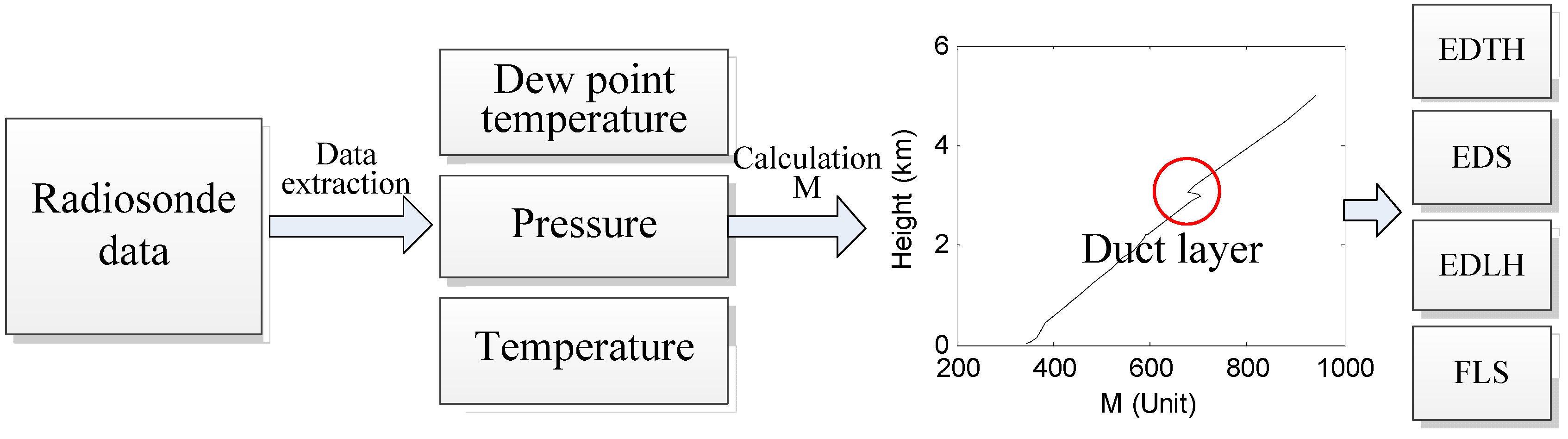
2.1.2. Method for Obtaining Atmospheric Duct Parameters
One of the most accurate methods for obtaining atmospheric duct parameters is radiosonde data. Radiosonde data were geopotential height, temperature, dew point temperature, wind direction, and wind speed observations during daily routine observation hours (00.00 and 12.00 universal time). There are approximately 600 high-altitude meteorological stations worldwide, and their distribution is shown in
Figure 4.
A flow chart of the atmospheric duct parameters calculation is shown in
Figure 5. The atmospheric modified refractive index profile is calculated using the height, temperature, atmospheric pressure, and dew point temperature data to determine the atmospheric duct presence and calculate the atmospheric duct parameters.
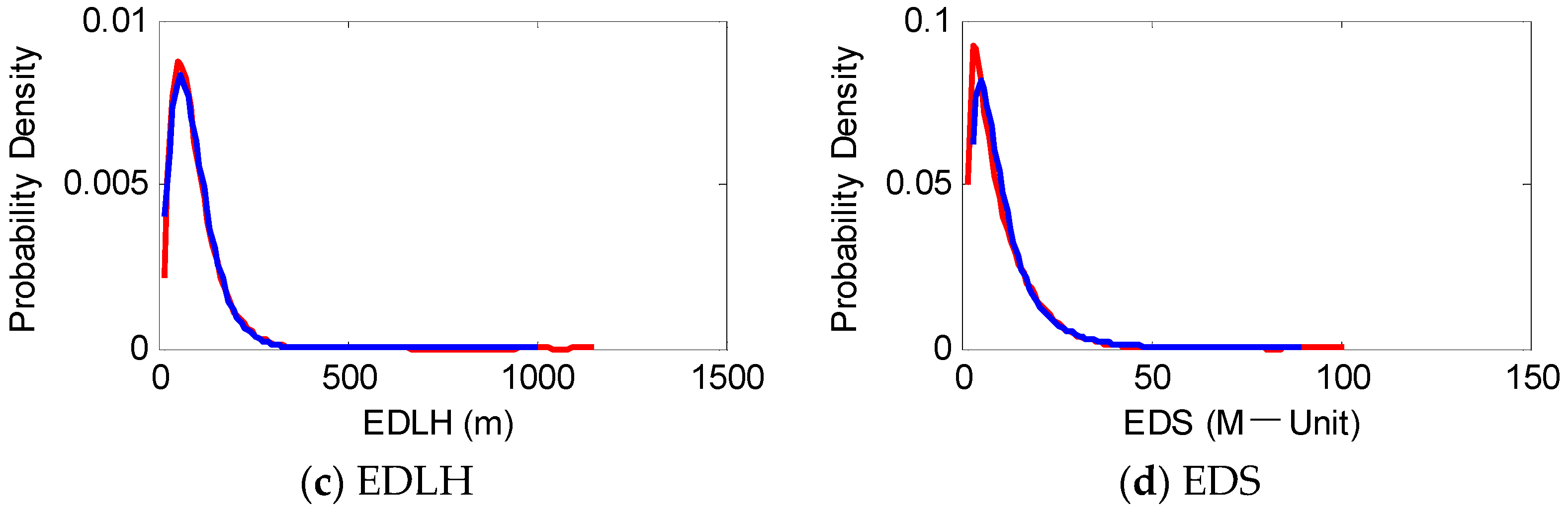
In this study, the atmospheric duct parameters were calculated using radiosonde data from 2015 to 2019, and the distribution of each parameter was fitted.
Figure 6 compares the probability density functions of the atmospheric duct parameters and the fitted probability density functions. The red line is the probability density curve, calculated using the measured elevated duct, and the blue line is the probability density curve obtained after fitting. EDTH and EDLH follow a gamma distribution, FLS and EDS follow a log-normal distribution. Atmospheric duct distribution parameters are listed in
Table 1.
2.2. Atmospheric Duct Parameters Sampling
The atmospheric duct parameter sample matrix was obtained using the Latin Hypercube Sampling (LHS) and rank correlation methods by fully considering the probability density distribution of atmospheric duct parameters and the correlation between parameters.
2.2.1. Sampling Method of Atmospheric Duct Parameters
The Latin Hypercube Sampling (LHS) Method is an approximate random sampling method [
15]. It can accurately reconstruct the atmospheric duct parameter distribution by sampling fewer iterations. The key to the LHS is to divide the atmospheric duct parameters cumulative probability distribution into intervals with equal probability and randomly select atmospheric duct parameter samples from each interval, thus, ensuring that the atmospheric duct parameter samples structure is similar to the overall structure, improving the estimation accuracy. The LHS method schematic is shown in
Figure 7.
The LHS steps are as follows:
The duct parameter cumulative distribution function is split into non-overlapping intervals of equal marginal probability ();
One of the intervals is randomly selected;
A value is randomly selected within the time interval to calculate the inverse distribution as the sample value of the first atmospheric duct parameter [
16];
The unselected interval is randomly selected to obtain samples in other iterative processes;
Repeat steps 1–4 for each atmospheric duct parameter.
2.2.2. Rank Order Correlation
Each parameter was sampled independently during the sampling atmospheric duct parameter process, using the LHS method. Consequently, the correlation between atmospheric duct parameters was disregarded in the sampling process. Therefore, to reproduce the duct parameters correlation characteristics in the sampling process and accurately describe the distribution of atmospheric duct parameters, it is necessary to introduce the desired correlation structure into the samples.
The study presents a method based on rank correlations intended to induce the desired rank dependence among input variables. Iman and Conover [
17] developed the input samples correlation technique based on the premise that rank correlation defines dependencies among input variables. Thus, a correlation coefficient computed on raw data may lose meaning and interpretability with non-normal data or in the presence of outliers. However, rank correlation coefficients are meaningful in most modeling situations, even when the data are normal.
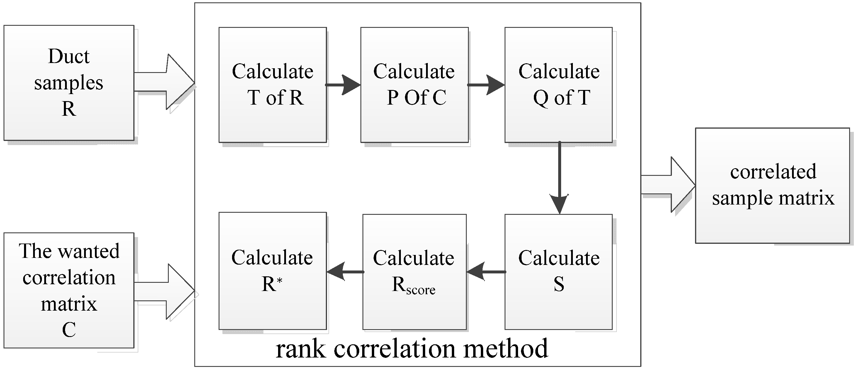
A flow chart of the rank correlation method is shown in
Figure 8, and the algorithm can be summarized in the steps outlined below:
Calculate of . is the correlation coefficient matrix of , and is the atmospheric duct parameters sample matrix; samples were approximately 4000, and the atmospheric duct parameters included EDTH, FLS, EDS, and EDLH;
Calculate the lower triangular Cholesky decomposition P of , where . is the matrix corresponding to the wanted correlation matrix;
Calculate the lower triangular Cholesky decomposition of , that is , where is the calculation result of step 1;
Obtain such that ; S can be calculated as ;
Obtain by rank-transforming and convert to van der Waerden scores;
Calculate the target correlation matrix , where ;
Match up the rank pairing in according to .
Based on the distribution of atmospheric duct parameters, approximately 4000 atmospheric duct parameter samples were obtained by the LHS method.
Considering EDTH as an example, LHS and random sampling were adopted. A comparison between the EDTH sample probability density distribution (obtained using LHS and random sampling) and the EDTH probability density distribution is shown in
Figure 9. Evidently, the probability density curve obtained using the random sampling method differed from the actual distribution, whereas the probability density distribution obtained using LHS exhibited a close fit to the actual distribution.
2.3. GNSS Occultation Signal Power Simulation
The GNSS occultation signal is divided into space- and ground-based occultation signals. The global atmospheric environment can be retrieved using space-based signals [
18,
19]; however, the accuracy is low when estimating the hyper-refraction environment in low-altitude atmospheric duct environments [
20,
21,
22]. Ground-based occultation signals can be used to estimate atmospheric environmental parameters [
23,
24,
25]. Therefore, in this paper, GNSS occultation data were used to invert atmospheric duct parameters.
The GNSS signal propagation model uses the reciprocity theorem to set the ground receiver as the transmitting source. The method avoids the top input field calculation, and the results are more reliable. The parabolic equation model is used to calculate the radio wave propagation factor in the atmospheric duct region, and the propagation factors in other regions remain unchanged [
25].
The path loss of the GNSS signal expressed in dB at elevation
is:
where
is the path propagation loss,
is the distance from the receiver to the satellite,
is the frequency, and
is the propagation factor calculated according to the parabolic equation.
Based on the GNSS signal power simulation algorithm and atmospheric duct parameter samples, GNSS signal power under different atmospheric duct conditions was calculated. The GNSS signal power variation with an elevation under different atmospheric duct parameters is shown in
Figure 10. The atmospheric duct parameters had a considerable impact on the GNSS signal power.
2.4. Global Sensitivity Analysis
Sensitivity analysis analyzes how the variation in the output of a model can be qualitatively or quantitatively apportioned to different variation sources and how a given model depends on the information fed into it [
26]. In this study, sensitivity analysis was primarily applied to the influence of different atmospheric duct parameters on the GNSS signal power.
The EFAST method is a global sensitivity analysis method proposed by Sailtelli et al., which combines the advantages of the Sobel method and the FAST. The method adopts the model variance analysis idea. It considers that the model output variance is caused by various input parameters and the interaction between them, reflecting the model output sensitivity to input parameters. Therefore, the contribution proportion of each parameter and the connection between parameters to the total variance can be obtained through the model variance decomposition; this is the parameter sensitivity index.
The EFAST method is a quantitative global sensitivity analysis method based on variance; that is, we consider that the variance of the model results can reflect the model output sensitivity results. In this method, the model sensitivity is divided into (1) the independent action sensitivity of a single parameter and (2) the sensitivity of the interaction between various parameters.
The model expression for the influence of atmospheric duct parameters on the GNSS signal power is:
where
is the input atmospheric duct parameters, and
is the change in GNSS signal power.
We selected an appropriate conversion function
to convert
to
. Here, the conversion function
is related to the probability density function of the parameter
:
where
is a scalar, and
and
are integer frequencies defined by the atmospheric duct parameters
.
Then, the change in variance caused by the atmospheric duct parameters is the sum of the squares of the integral multiples of
amplitudes, that is,
The total variance of the model and the first-order variance caused by the atmospheric duct parameters can be calculated using Equations (9)–(11). According to Equation (12), the main sensitivity index of atmospheric duct parameters after ignoring the coupling with other parameters can be calculated as follows:
where
is the atmospheric duct parameters total sensitivity index; that is, the sum of the sensitivity indices of each order, which can be expressed as:
Figure 11 shows the atmospheric duct parameters sensitivity calculated using the EFAST method. FLS has the highest sensitivity and the greatest impact on the GNSS signal power distribution; the EDTH, EDLH, and EDS sensitivities were similar. The total sensitivity index of all parameters was large. The main sensitivity index was different from the total sensitivity index. It can be inferred that there is a strong correlation between the different input parameters.
Based on the global sensitivity analysis results, the total sensitivity index was selected as the weight coefficient.
4. Results and Discussion
Different atmospheric duct inversion models are established using the traditional and proposed loss functions. The comparison of inversion results is shown in
Figure 14. A sample is randomly selected from the validation set as a reference sample.
Figure 14 shows that the atmospheric duct inversion result was closer to the reference value after applying our proposed loss function. To statistically analyze the influence of different loss functions on the atmospheric duct inversion results, we used the validation set data to calculate the atmospheric duct inversion accuracy.
We used the mean absolute percentage error (MAPE), mean absolute error (MAE), and root means square error (RMSE) to evaluate the accuracy of duct parameter inversion results.
Table 3 compares the atmospheric duct parameters inversion results using the traditional loss function and our proposed loss function. Furthermore,
Table 3 shows that the RMSE, MAE, and MAPE calculated using our proposed loss function were less than the traditional loss function, indicating that the loss function was more suitable for atmospheric duct parameter inversion.
White Gaussian noise was added to the deep learning data set to evaluate the atmospheric duct inversion model performance in the case of noise pollution.
Table 4 shows the atmospheric duct inversion results under white Gaussian noise conditions. Furthermore,
Table 4 shows that after adding noise in the training set, the inversion accuracy of atmospheric duct parameters using different loss functions was reduced. However, the inversion accuracy using the loss function proposed was better than that using the traditional loss function, showing that the loss function proposed yielded better stability and anti-noise ability.
Our model has higher accuracy and improved applicability than the traditional method regarding the inversion of duct parameters. Furthermore, our experimental results show that an appropriate loss function can effectively improve the performance of deep learning networks.


