Article

Spatial Downscaling of GOES-R Land Surface Temperature over Urban Regions: A Case Study for New York City

1
The Graduate Center, City University of New York, New York, NY 10016, USA
2
New York City College of Technology, City University of New York, Brooklyn, New York, NY 11201, USA
3
India Meteorological Department, Ministry of Earth Sciences, New Delhi 110003, India
4
City College of New York, City University of New York, Manhattan, New York, NY 10031, USA
5
NASA Goddard Institute for Space Studies, New York, NY 10025, USA
*
Author to whom correspondence should be addressed.
Atmosphere 2022, 13(2), 332; https://doi.org/10.3390/atmos13020332
Submission received: 21 December 2021 / Revised: 11 February 2022 / Accepted: 12 February 2022 / Published: 16 February 2022
(This article belongs to the Special Issue Remote Sensing and GIS Applications in Urban Climate Research)

Abstract

:
The surface urban heat island (SUHI) effect is among the major environmental issues encountered in urban regions. To better predict the dynamics of the SUHI and its impacts on extreme heat events, an accurate characterization of the surface energy balance in urban regions is needed. However, the ability to improve understanding of the surface energy balance is limited by the heterogeneity of surfaces in urban areas. This study aims to enhance the understanding of the urban surface energy budget through an innovation in the use of land surface temperature (LST) observations from remote sensing satellites. A LST database with 5–min temporal and 30–m spatial resolution is developed by spatial downscaling of the Geostationary Operational Environmental Satellites—R (GOES–R) series LST product over New York City (NYC). The new downscaling method, known as the Spatial Downscaling Method (SDM), benefits from the fine spatial resolution of Landsat–8 and high temporal resolution of GOES–R, and considers the temporal variation in LST for each land cover type separately. Preliminary results show that the SDM can reproduce the temporal and spatial variability of LST over NYC reasonably well and the downscaled LST has a spatial root mean square error (RMSE) of the order of 2 K as compared to the independent Landsat–8 observations. The SDM shows smaller RMSE of 1.93 K over the tree canopy land cover, whereas RMSE is 2.19 K for built–up areas. The overall results indicate that the SDM has potential to estimate LST at finer spatial and temporal scales over urban regions.

1. Introduction

Reliable estimates of land surface temperature (LST) are crucial for understanding the land–atmosphere energy budget, hydrological and biogeochemical cycles, climate change, as well as for land surface model data assimilation [1,2,3,4]. LST is also a key input variable for the estimation of land surface emissivity, evapotranspiration, and latent and sensible heat fluxes [5,6,7]. Differences in LST and near–surface air temperature are often difficult to characterize because LST exhibits different patterns of spatial and temporal variability than near–surface air temperature over a specific region [8].
Further, in–situ observations of LST are not uniform everywhere, and that hinders applicability due to limited spatial representation. On the other hand, satellite remote sensing provides LST estimates at uniform spatial and temporal scales globally or quasi–globally. Thermal infrared (TIR) sensors provide LST estimates at finer spatial resolution with reasonable accuracy, but they are restricted to clear–sky conditions alone. An example of one of the most widely used TIR–based LST products is obtained from the Moderate Resolution Imaging Spectroradiometer (MODIS) derived LST estimates, and it has been successfully used for numerous applications worldwide [3,4,8,9,10,11]. Microwave sensors provide LST estimates for all–weather conditions, but their spatial resolution is rather coarse. Hence, integration of both TIR– and microwave–based LST estimates could provide better estimates of LST for all–weather conditions at finer spatial and temporal scales [12,13].
Satellite–based LST estimates have been widely used for the study of surface urban heat island (SUHI) intensity and changes in their spatial extent [2,14,15,16,17]. The SUHI phenomenon is generally seen as being caused by a reduction in latent heat flux and an increase in sensible heat flux in urban areas as vegetated and evaporating soil surfaces are replaced by relatively impervious low albedo paving and building materials. However, the adequate monitoring of SUHI requires high temporal (~10–15 min) and spatial resolution (~50–100 m) LST estimates.
LST estimates from the polar–orbiting satellites such as the Landsat satellite series are optimal for SUHI studies due to finer spatial resolution (e.g., 30 m derived from the native 100 m spatial resolution of Landsat–8) and good radiometric accuracy [18]. However, their long revisit time (~16 days), rather narrow swath, and non–availability of data in the presence of clouds restrict their use. In contrast, geostationary satellites such as the Geostationary Operational Environmental Satellites–R (GOES–R) series provides LST estimates over a specific region very frequently (e.g., every 5 min) to monitor diurnal variability, but at a rather coarse spatial resolution of about 2 km [19,20]. Overall, there is not one single TIR–based satellite sensor capable of producing LST estimates at both finer spatial and temporal scales.
The generation of fine spatiotemporal resolution LST data for urban areas is promising, and several methods have been proposed for the downscaling of satellite–based LST estimates over urban regions through physical or statistical methods for SUHI monitoring and other applications (e.g., [12,21,22,23,24,25,26,27,28,29,30,31]). Bechtel et al. [21] used a downscaling approach based on several predictors to downscale TIR–based LST estimates from a geostationary satellite and showed that the method was able to downscale LST for a factor of about 2000 with an accuracy of the order of 2 K. Weng et al. [23] proposed a spatiotemporal adaptive data fusion algorithm for temperature mapping to obtain finer resolution LST by blending daily MODIS and periodic Landsat datasets over Los Angeles County, California, USA, and an accuracy of 1.3–2 K was reported. However, this model was unable to predict changes in LST due to limitations in model assumptions. Wu et al. [12] developed a spatiotemporal integrated temperature fusion model for the synergism of LST from multi–scale polar–orbiting and geostationary satellite datasets in a unified framework, and an independent validation of the fused LST showed accuracy of about 2.5 K. Bonafoni [24] suggested a statistical downscaling method based on relationships between LST and about 10 spectral indices to downscale LST estimates from Landsat and MODIS sensors over the city of Milan, Italy. They suggested that the combined use of vegetation and built–up/soil indices would be advantageous for LST downscaling procedures over heterogeneous urban landscapes. Further, GOES –derived LST imagery at 4 km was spatially downscaled to 1 km for Los Angeles, USA using geospatial and census data to characterize and quantify heat hazard [30]. It was shown that spatial downscaling methods with geostationary LST imageries enable the study of the diurnal cycle of SUHI [22,31]. However, these studies use several parameters as inputs, with uncertainties in each input parameter propagating throughout the downscaled LST product. It is to be noted that correct spatiotemporal features must be reproduced after applying downscaling techniques for SUHI studies [25]. Additionally, the relationship of fine and coarse resolution data varies diurnally, which could not be captured adequately using a static downscaling approach. Comprehensive reviews of advancement in LST downscaling methods (both spatially and temporally) along with their advantages and limitations were recently outlined by Mao et al. [32] and Wu et al. [33].
The objective of this study is to generate a high spatial (30 × 30 m) and temporal (5–min) resolution LST dataset by the combined use of Landsat–8 and GOES–R products for SUHI studies. Several studies independently focused on improving the LST retrievals from different satellites. However, here our main goal is to develop a method to enhance their spatial and temporal variabilities. The proposed downscaling method, known as the Spatial Downscaling Method (SDM), not only benefits from the relative merits of Landsat–8 and GOES–R, but also considers the temporal variation in LST for each land cover (LC) type separately. This proposed method is primarily tested over the New York City (NYC) region of the USA as a preliminary analysis.

2. Study Area and Datasets
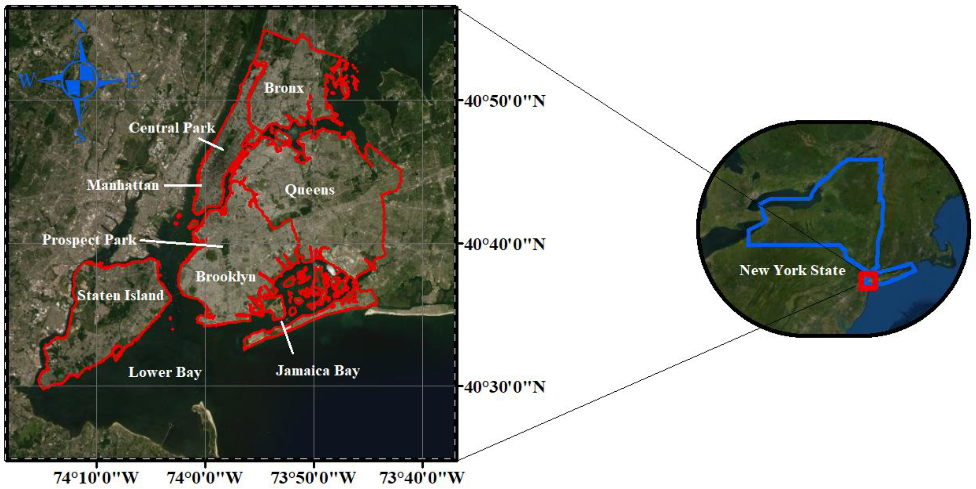
2.1. Study Area

The study area comprises NYC (Figure 1), a region with a population of about 8.5 million people. The city has an average altitude of 10 m, and its center is located at 40°43′50.1960″ N and 73°56′6.8712″ W. The study area covers the five boroughs of NYC, namely Bronx, Brooklyn, Manhattan, Queens, and Staten Island. The city consists of a range of LC including tree canopy, grass/shrub, bare land, water, buildings, roads and others paved surfaces as identified by the 2010 New York City Open Data resource provided by the Department of Parks and Recreation (https://data.cityofnewyork.us/Environment/Landcover-Raster-Data-2010-3ft-Resolution/9auy-76zt (accessed on 10 September 2021)). This LC dataset is derived from the combined use of 2010 Light Detection and Ranging (LiDAR), 2008 four-band orthoimagery, and ancillary geospatial datasets through the object–based image analysis method. This dataset was developed as part of the Urban Tree Canopy Assessment for New York City and overall accuracy of 96% was reported. The spatial distribution of the major LC types over NYC at 30 m spatial resolution is shown in Figure 2a.
A heat island effect exists in NYC, with the mean temperatures at Central Park generally being 1.20–3.02 °C lower than the surrounding temperatures, and the surface air temperature of the city is up to 8 °C warmer than the rural areas within 100 km of the city and the difference becomes more pronounced during heat wave conditions [34,35]. For instance, the urban heat island intensity was observed to be nearly twice in July 2016 over NYC compared to the decadal mean [35].
The 3ft–resolution LC raster file was upscaled to 30 m and 2 km to match the spatial resolution of Landsat–8 and GOES–R LST data, respectively. For each resampling case, the upscaled pixel was obtained by selecting the most frequent LC from the nearest original LC pixels. At 3–ft resolution, the LC data is composed of seven land classes that include tree canopy, grass/shrub, bare soil, water, buildings, roads/railroads, and other paved surfaces. The upscaled 30 m resolution LC is composed of four classes namely, tree canopy, grass/shrub, water, and buildings (e.g., Figure 2a). When LC dataset is upscaled from 30 m resolution to 2 km resolution, the most frequent LC classes are tree canopy, grass/shrub, and buildings. These three LC classes were used to construct the LST diurnal cycle of the GOES–R for the month of July in 2017 as shown in Figure 2b.

2.2. Landsat–8 Data

Landsat images offer the longest continuous global record of the Earth’s surface. Since 1972, they have been unique resources for the global change research and applications in agriculture, cartography, geology, forestry, regional planning, surveillance, education, and national security [18,36]. Landsat–8 was launched on 11 February 2013 and has a minimum of 16 days revisit cycle, which is sometimes extended due to cloud contamination. The satellite has 11 bands having a spatial resolution of 15–100 m, and they are available from the United States Geological Survey (USGS) website (https://earthexplorer.usgs.gov/ (accessed on 10 September 2021)). Landsat–8 LST is retrieved using a generalized single–channel method from the Landsat TIRS 1 (Band 10) within the range of 10.6–11.2 µm, because large calibration uncertainty in TIRS band 11 since 2014 was reported by the USGS [37,38]. The surface emissivity, atmospheric transmittance, and effective mean atmospheric temperatures are three essential parameters that need to be computed for the LST retrieval from the Landsat single TIRS band data [38]. Level 1 product from the band 10 is converted into spectral radiance using the radiance scaling factors provided with the metadata (Equation (1)).
Lλ = ML × Qcal + AL
where, Lλ is the spectral radiance, ML is the radiance multiplicative rescaling factor, Qcal is the Level–1 pixel value in digital number, and AL is the radiance additive rescaling factor. As the USGS has reprocessed the TIRS band 10 data including radiance offsets, calibration offset is not introduced in Equation (1).
The spectral radiance is then converted into brightness temperature (Tb) through the approximation of the Planck radiance function and given by
Tb = K2/ln(K1/Lλ + 1)
where, K1 and K2 are band–specific thermal conversion constants provided with the metadata and given in Table 1. The unit of resultant Tb is Kelvin.
Finally, Tb is divided by the surface emissivity ε to obtain LST using Equation (3).
LST = Tb/ε
As for the surface emissivity, we applied a universal value for all urban surfaces. Several studies have shown that the approximate value of emissivity in urban areas ranges from 0.96 to 0.99. We used a widely accepted value in the literature for urban built areas in very densely populated cities of ε = 0.99 [39,40,41]. Based on our sensitivity analysis, every 0.01 surface emissivity difference will change the absolute value of LST by about 0.75 K. Landsat–8 provides one of the finest spatial resolution satellite–based LST estimates to monitor urban growth and the SUHI. However, the presence of clouds, aerosols, and diverse spatial distributions of water vapor content highly disturbs the process of acquisition. The thermal band 10 of Landsat–8 has a 100 m native spatial resolution, but is resampled and published at 30 m by the USGS. Hence, the spatial resolution of Landsat–8 derived LST is 30 m. In order to ensure the use of high–quality data for the downscaling, we discarded data that have more than 10% of cloud coverage from July 2017 to April 2018. The details of Landsat–8 images along with magnitudes of rescaling factors and thermal constant values used for LST estimation over NYC are provided in Table 1.

2.3. GOES–R Data

The Geostationary Operational Environmental Satellites (GOES) are a series of geostationary satellites operated by the National Oceanic and Administration (NOAA)/National Environmental Satellite, Data and Information Service (NESDIS) for weather nowcasting, meteorology and climate research of the Western Hemisphere. The primary instrument on the GOES–R series launched in 2016 is the Advanced Baseline Imager (ABI) with its 16 different spectral bands; the bands are composed of two visible channels, four near–infrared channels, and 10 infrared channels [42]. The LST product from the ABI is based on a split–window technique that corrects for atmospheric absorption and applies surface prescribed emissivity information. In addition, an atmospheric path length term is applied to further correct the satellite view zenith angle effect. Coefficients of the LST algorithm, which were derived using an atmospheric radiative transfer model, are stratified for daytime and nighttime conditions, as well as for dry and moist atmospheres. The algorithm is then verified using a radiative transfer simulation dataset and evaluated using proxy dataset and ground measurements [19,43]. The accuracy of the GOES–R LST products is found to be about 2.5 K, and that meets the mission requirements [20]. A comparison of diurnal variations in LST from the GOES–R ABI and MODIS sensors over North America showed a general agreement with each–other except for the mountainous regions [44]. LST data at 5 –min temporal resolution and about 2 km spatial resolution over the Continental United States were obtained from the NOAA for 2017 and 2018.

3. Spatial Downscaling Method (SDM)

All concurrent Landsat–8 and GOES–R LST products over NYC between 2017 and 2018 were collected. First of all, concurrent Landsat–8 data were re–projected from the Universal Traverse Mercator to Geographical Coordinate System to match the GOES–R spatial grid. Using both GOES–R and Landsat–8 LSTs observed at the same date and time, their spatial relationship was found through a linear regression model. This statistical method considers the differences between the sensors and accounts for their seasonal changes. Then, the SDM is applied to sharpen the GOES–R data. The structure of the SDM is presented below in Equation (4).
T(x, y, t) = TG(X, Y, t) + ΔTL(x, y) + T(GL)(X, Y) + ΔTG(T) + ΔT(GdownscaledL)
where,
  • t stands for 5–min time intervals
  • T stands for averaged diurnal time of Landsat–8 observations
  • x and y stand for the location of 30 m pixel (Landsat–8 pixel)
  • X and Y stand for the location of 2 km pixel (GOES–R pixel)
  • G stands for GOES–R
  • L stands for Landsat–8.
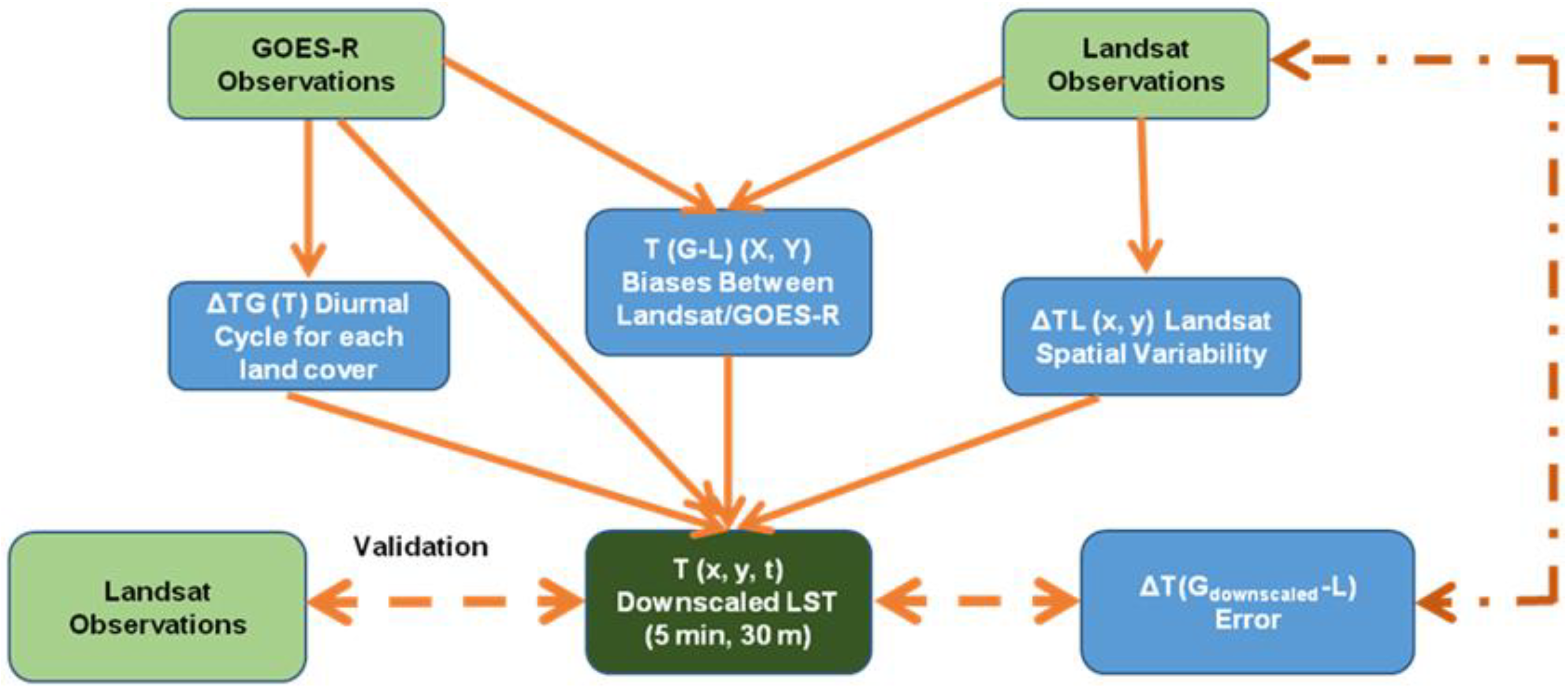
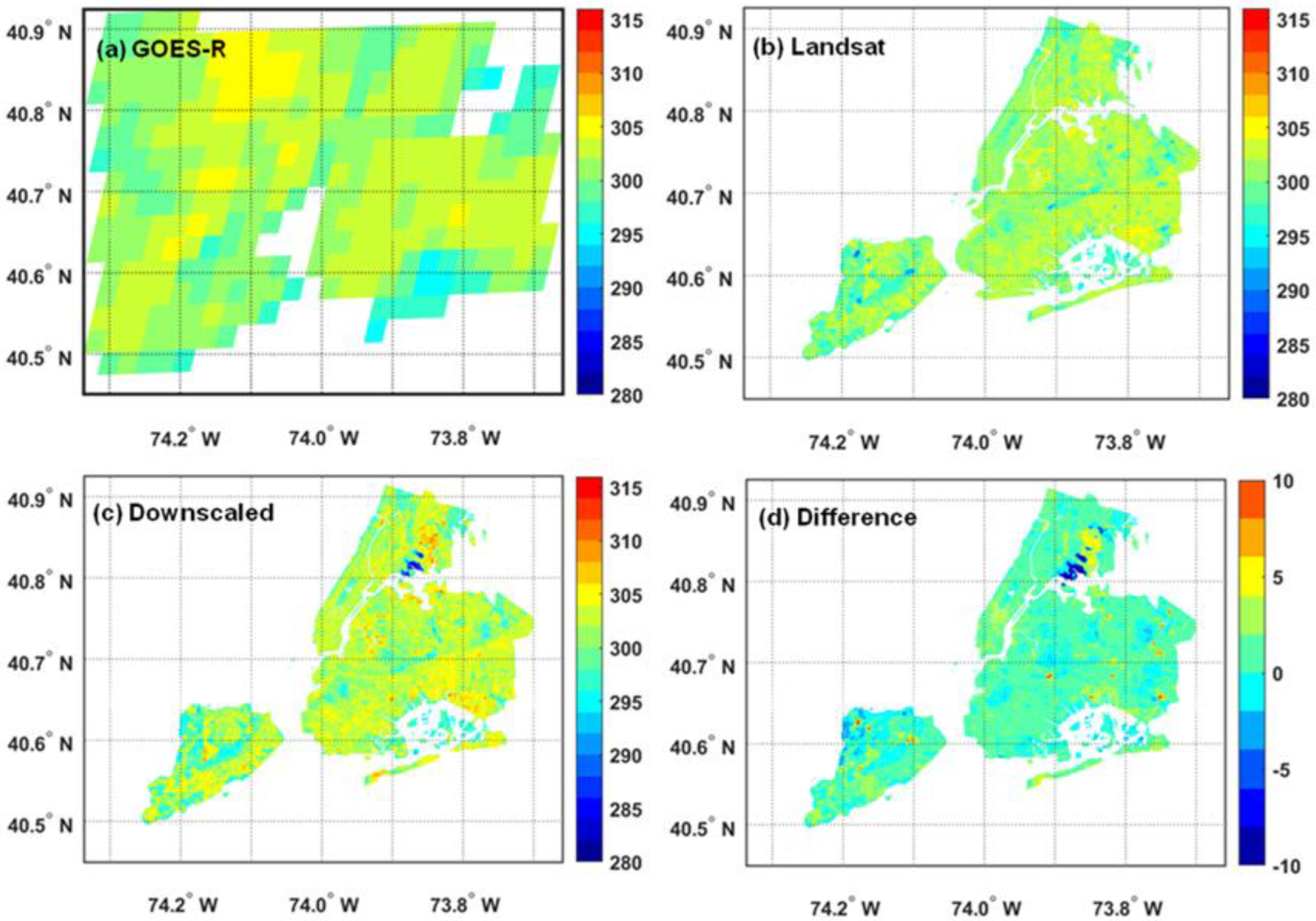
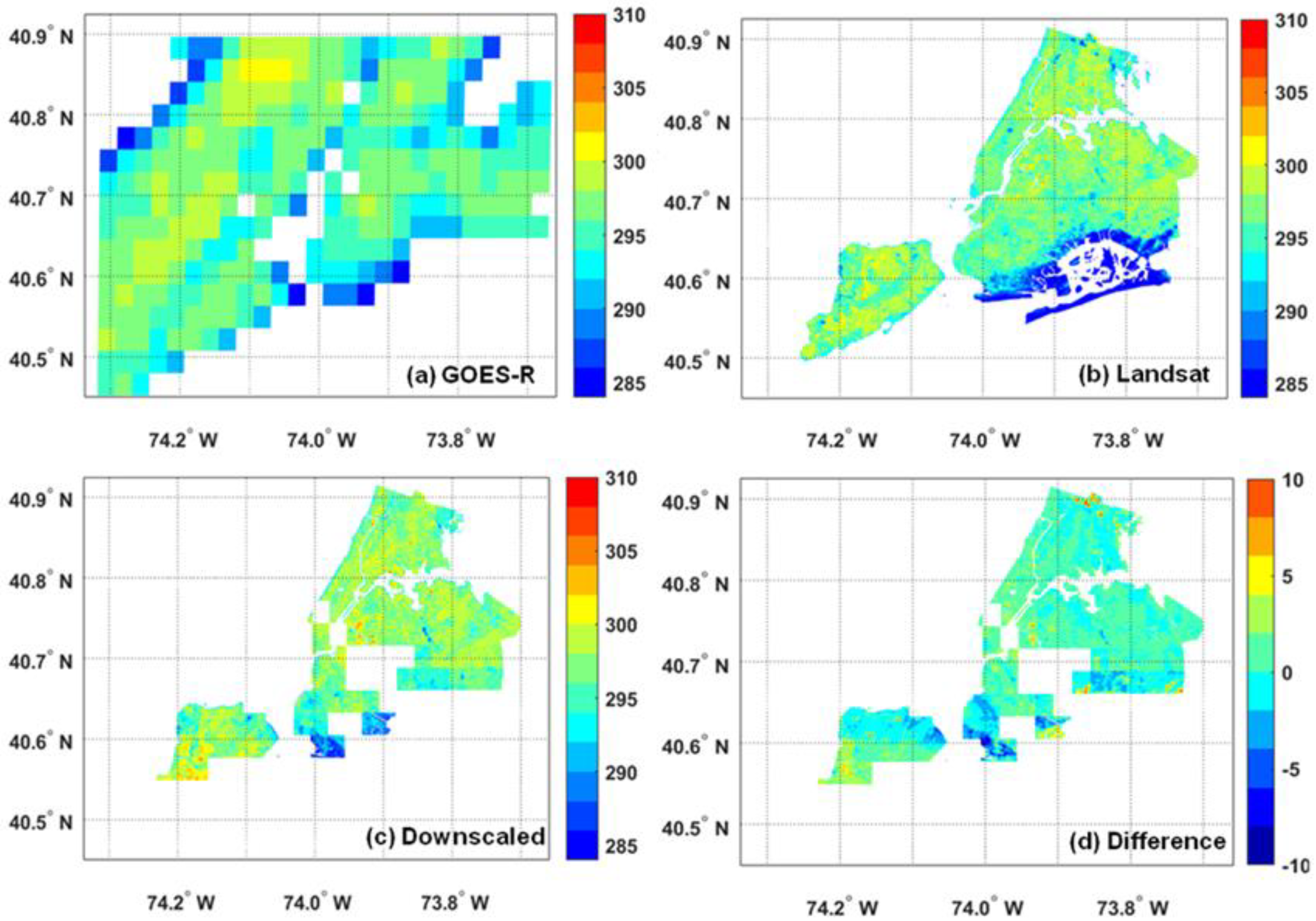
  • T(x, y, t) is the GOES–R downscaled LST to Landsat–8 resolution (30 m)
  • TG(X, Y, t) is the observed GOES–R temperature at coarser resolution
  • ΔTL(x, y) is the spatial variability of each Landsat–8 pixel with respect to the averaged Landsat–8 LST pixel, which is obtained by removing the mean LST value from each LST pixel of Landsat–8.
  • T(G − L)(X, Y): there is a systematic bias between Landsat–8 and GOES–R in LST measurements even for the same time and spatial scales due to sensor configurations, footprint size, radiometric and spectral differences, and retrieval algorithms. These systematic differences are accounted for by removing the average of Landsat–8 LST from the GOES–R LST measurements. This bias is represented in the equation by T(GL)(X, Y).
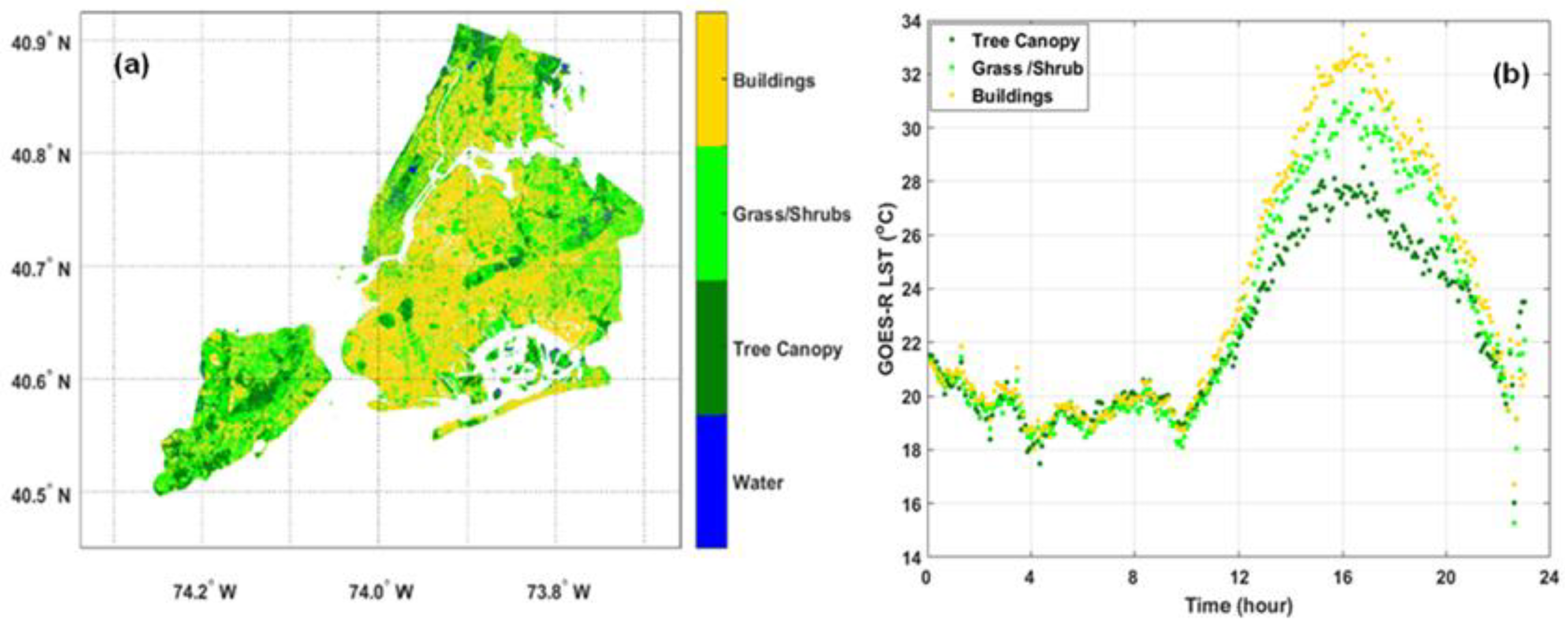
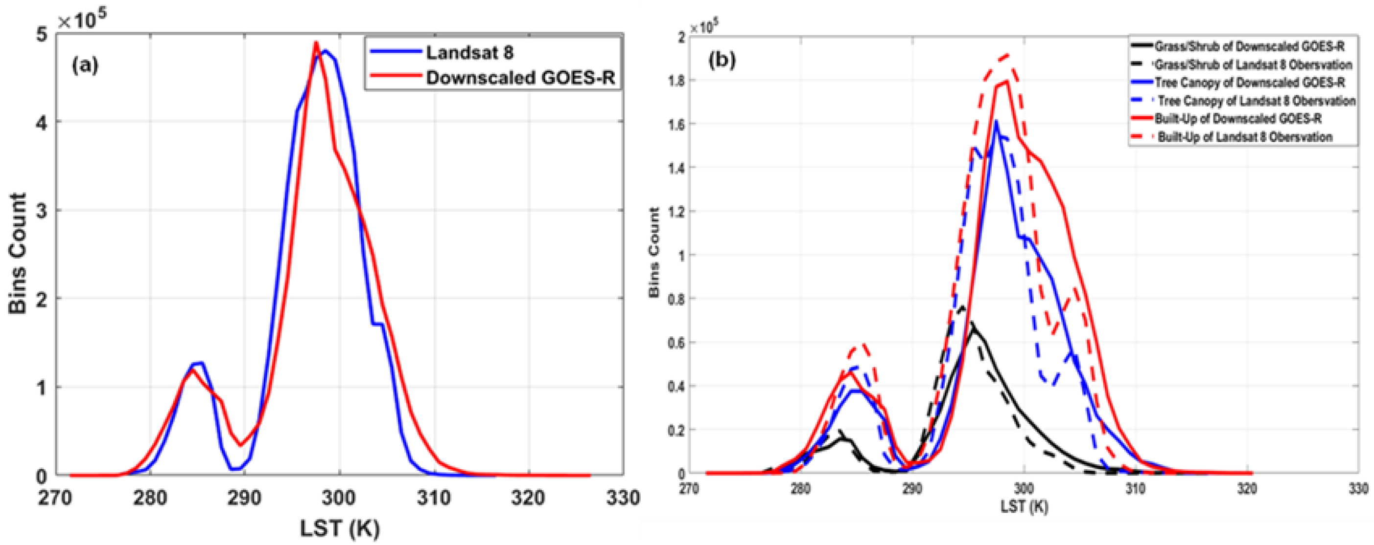
  • ΔTG(T): the temporal differences between LC types at finer resolutions are accounted for by the GOES–R diurnal LST variability, ΔTG(T). This term is calculated based on monthly diurnal variability and each LC type that is obtained from a 30 m resolution of NYC land cover map and then re–sampled to 2 km resolution the same as the GOES–R. The term ΔTG(T) is the temperature of each LC class at every 5–min subtracted by the temperature of LC class at a time that ranges between 11:30 a.m. and 11:40 a.m.
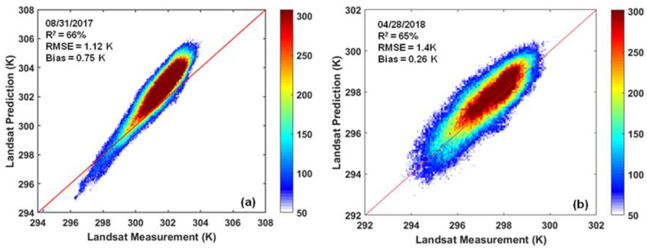
  • ΔT(Gdownscaled − L) represents the post–downscaling errors between downscaled GOES–R LST and Landsat–8 LST observations.
Figure 2b represents the average LST values at 5–min intervals for major LC types in the NYC area (i.e., tree canopy, grass/shrub, and buildings) using GOES–R observations for July 2017. The LST values are reaching their maximum between 4:00 p.m. and 5:00 p.m. local solar time, and buildings show higher magnitude of diurnal temperature variability as expected compared to trees and grass surfaces. The considerable dependence of LST variability on LC type is reported in the recent studies e.g., [9,11]. The entangled succession of operations is illustrated in the accompanying flowchart shown in Figure 3.
Furthermore, eight independent Landsat–8 images (e.g., which are not the part of SDM) between 2017 and 2018 were used for the evaluation of the SDM over NYC. The widely used statistical metrics such as correlation coefficient (square root of coefficient of determination), bias and root mean square error (RMSE) were used for the evaluation of the downscaled LST against independent Landsat–8 LST datasets.

4. Results and Discussion

Using the SDM, GOES–R LST observations were downscaled to Landsat–8 spatial resolution level for every 5–min over NYC. The results were compared with eight independent Landsat–8 LST observations. However, we present only two case studies here for brevity. Figure 4 shows the spatial distributions of observed GOES–R LST, Landsat–8 LST, downscaled LST, and difference between SDM and Landsat–8 LST for 31 August 2017. This corresponds to the summer LST for the city. It is to be noted that the independent Landsat–8 LST dataset is considered as a reference to compare the potential of SDM. The overall spatial patterns of downscaled and observed LSTs match appreciably well. As expected, LST over the built–up areas is higher than the vegetated areas. The difference between SDM and Landsat–8 observations is usually less than 2 K.
Figure 5 shows the spatial distributions of observed GOES–R LST, Landsat–8 LST, downscaled LST, and difference between SDM and Landsat–8 LST for 28 April 2018. The southeastern part of the city shows rather less LST as compared to other parts of the city using the Landsat–8 dataset.
However, the SDM provides missing values over some parts of the city due to the non–availability of the GOES–R dataset. The spatial patterns of the SDM LST are in good agreement with the Landsat–8 dataset. LST variations with LC types are also preserved by the SDM, and the unique LST patterns in buildings can be discerned. The SDM overestimates LST over large parts of the study area and underestimates by about 2–3 K as compared to the Landsat–8 observations over some parts of NYC. In addition, bias in the downscaled LST shows a considerable seasonal variation with the largest magnitude of bias occurring during fall and the smallest magnitude of bias occurring during winter. This analysis clearly reveals that the SDM can reproduce the spatial variability of LST over NYC.
Figure 6 presents the quantitative comparison of the downscaled LST with Landsat–8 observations over NYC for 31 August 2017 and 28 April 2018. In both cases, the coefficient of determination is quite high (65–66%) which suggests that the downscaled LST obtained from the GOES–R and Landsat–8 correlated quite well. The data points fall close to the diagonal line, indicating that the downscaled LST are in good agreement with the observations. Although SDM marginally overestimates LST as compared to Landsat–8 observations, the bias is 0.75 K for 31 August 2017, whereas it is as low as 0.26 K for 28 April 2018. The general overestimation of LST by GOES–R as compared to Landsat–8 was also observed over North America [44]. The root–mean–square error (RMSE) in the SDM LST is less than 1.5 K in both cases. These error metrics again show that SDM has the potential to downscale GOES–R LST over the urban region with reasonable accuracy. Nonetheless, such analysis was undertaken for several cases across NYC for different seasons. The coefficient of determination varies between 0.49 and 0.87, whereas RMSE is usually less than 2 K for all cases. The overall error metrics for the SDM for three distinct LC types across NYC are provided in Table 2.
The SDM shows high correlation coefficients of 0.73–0.75 as compared to the Landsat–8 dataset for these three LC types. The SDM shows smallest RMSE of 1.93 K over the tree canopy LC, whereas RMSE is 2.19 K for built–up areas. The differences in RMSEs for different LC types might be associated with their respective LST variability. For instance, built–up area shows the largest diurnal variability, whereas tree cover area has the smallest diurnal variability across NYC (e.g., Figure 2b).
Figure 7a illustrates the histogram of LST from SDM and Landsat–8 for NYC. The histograms show the general LST distribution. The LST data have bimodal distributions and the histograms tend to center closer to 300 K in both products.
The bimodal distributions of LST are due to seasonal variations in LST (e.g., summer and winter seasons). The histogram of LST from SDM and Landsat–8 for three different LC types over NYC is presented in Figure 7b. The histograms of LST are quite similar for Landsat–8 and downscaled GOES–R for three LC types. However, the downscaled GOES–R LST shows marginally higher values in LST when compared to the observed Landsat–8. Several studies independently focused on improving the LST retrievals from different satellites. However, here our main goal is to develop a method to enhance their spatial and temporal variabilities. That means utilizing more accurate and improved retrieval methods also could improve the quality of the input data sets in the proposed method here. This downscaling method explicitly considers the effect of different LC types on LST distribution. This preliminary analysis clearly indicates the potential of proposed SDM for GOES–R derived LST downscaling for SUHI studies. However, this study is planned to be extended with a longer period of the GOES–R dataset and a comprehensive evaluation against in–situ observations in continuation of this study. Furthermore, thermal infrared based LST datasets are available for clear sky conditions only, and a suitable method for gap filling is also needed to obtain a spatially consistent LST dataset over the urban environment.

5. Conclusions

This study proposed a downscaling model, SDM, for estimating LST at very high temporal and spatial resolution (e.g., 5–min and 30 m) using GOES–R datasets. The SDM algorithm generated LST with the consideration of its temporal variability with each LC class. This algorithm also benefits from the relative merits of frequent temporal sampling of GOES–R and fine spatial resolution of Landsat–8. A preliminary comparison over NYC with independent Landsat–8 observations showed general agreement between the SDM and Landsat–8 LST datasets with RMSE less than 2 K. The spatial variability of LST over the NYC was captured reasonably well by the downscaled LST. The overall results indicate that the SDM has potential to estimate LST at a finer spatial scale over urban regions for SUHI studies. However, there is a need to extensively validate the downscaled LST with ground–based observations over the city. This validation effort will be conducted in the near–future as a continuation of this study.

Author Contributions

Conceptualization, H.N., S.P. and R.B.; methodology, A.R.B. and H.N.; formal analysis, A.R.B.; writing—original draft preparation, A.R.B. and S.P.; writing—review and editing, H.N., R.B., R.K. and C.R.; supervision, H.N., R.B. and R.K. All authors have read and agreed to the published version of the manuscript.

Funding

This research was funded by the National Oceanic and Atmospheric Administration—Cooperative Science Center for Earth System Sciences and Remote Sensing Technologies (NOAA–CESSRST) under the Cooperative Agreement Grant NA16SEC4810008, and by the Center for Remote Sensing and Earth System Sciences at the New York City College of Technology.

Institutional Review Board Statement

Not applicable.

Informed Consent Statement

Not applicable.

Data Availability Statement

The landcover data was obtained form the 2010 New York City Open Data resource provided by the Department of Parks and Recreation (https://data.cityofnewyork.us/Environment/Landcover-Raster-Data-2010-3ft-Resolution/9auy-76zt, (accessed on 10 September 2021)). The Landsat data are available from the United States Geological Survey (USGS) website (https://earthexplorer.usgs.gov/, (accessed on 10 September 2021)).

Conflicts of Interest

The authors declare no conflict of interest. The funders had no role in the design of the study; in the collection, analyses, or interpretation of data; in the writing of the manuscript, or in the decision to publish the results.

References

  1. Li, Z.-L.; Tang, B.-H.; Wu, H.; Ren, H.; Yan, G.; Wan, Z.; Trigo, I.F.; Sobrino, J.A. Satellite–derived land surface temperature: Current status and perspectives. Remote Sens. Environ. 2013, 131, 14–37. [Google Scholar] [CrossRef] [Green Version]
  2. Zhou, D.; Xiao, J.; Bonafoni, S.; Berger, C.; Deilami, K.; Zhou, Y.; Frolking, S.; Yao, R.; Qiao, Z.; Sobrino, J.A. Satellite remote sensing of surface urban heat islands: Progress, challenges, and perspectives. Remote Sens. 2019, 11, 48. [Google Scholar] [CrossRef] [Green Version]
  3. Azarderakhsh, M.; Prakash, S.; Zhao, Y.; AghaKouchak, A. Satellite–based analysis of extreme land surface temperatures and diurnal variability across the hottest place on Earth. IEEE Geosci. Remote Sens. Lett. 2020, 17, 2025–2029. [Google Scholar] [CrossRef]
  4. Zhao, Y.; Norouzi, H.; Azarderakhsh, M.; AghaKouchak, A. Global patterns of hottest, coldest and extreme diurnal variability on Earth. Bull. Am. Meteorol. Soc. 2021, 102, E1672–E1681. [Google Scholar] [CrossRef]
  5. Kalma, J.D.; McVicar, T.R.; McCabe, M.F. Estimating land surface evaporation: A review of methods using remotely sensed surface temperature data. Surv. Geophys. 2008, 29, 421–469. [Google Scholar] [CrossRef]
  6. Norouzi, H.; Temimi, M.; Rossow, W.; Pearl, C.; Azarderakhsh, M.; Khanbilvardi, R. The sensitivity of land emissivity estimates from AMSR-E at C and X bands to surface properties. Hydrol. Earth Syst. Sci. 2011, 15, 3577–3589. [Google Scholar] [CrossRef] [Green Version]
  7. Prakash, S.; Norouzi, H.; Azarderakhsh, M.; Blake, R.; Prigent, C.; Khanbilvardi, R. Estimation of consistent global microwave land surface emissivity from AMSR-E and AMSR2 observations. J. Appl. Meteorol. Climatol. 2018, 57, 907–919. [Google Scholar] [CrossRef]
  8. Prakash, S.; Shati, F.; Norouzi, H.; Blake, R. Observed differences between near-surface air and skin temperatures using satellite and ground-based data. Theor. Appl. Climatol. 2019, 137, 587–600. [Google Scholar] [CrossRef]
  9. Sharifnezhadazizi, Z.; Norouzi, H.; Prakash, S.; Beale, C.; Khanbilvardi, R. A global analysis of land surface temperature diurnal cycle using MODIS observations. J. Appl. Meteorol. Climatol. 2019, 58, 1279–1291. [Google Scholar] [CrossRef]
  10. Wu, X.; Wang, G.; Yao, R.; Wang, L.; Yu, D.; Gui, X. Investigating surface urban heat islands in South America based on MODIS data from 2003–2016. Remote Sens. 2019, 11, 1212. [Google Scholar] [CrossRef] [Green Version]
  11. Prakash, S.; Norouzi, H. Land surface temperature variability across India: A remote sensing satellite perspective. Theor. Appl. Climatol. 2020, 139, 773–784. [Google Scholar] [CrossRef]
  12. Wu, P.; Shen, H.; Zhang, L.; Gottsche, F.-M. Integrated fusion of multi-scale polar-orbiting and geostationary satellite observations for the mapping of high spatial and temporal resolution land surface temperature. Remote Sens. Environ. 2015, 156, 169–181. [Google Scholar] [CrossRef]
  13. Sun, D.; Li, Y.; Zhan, X.; Houser, P.; Yang, C.; Chiu, L.; Yang, R. Land surface temperature derivation under all sky conditions through integrating AMSR-E/AMSR-2 and MODIS/GOES observations. Remote Sens. 2019, 11, 1704. [Google Scholar] [CrossRef] [Green Version]
  14. Gaffin, S.R.; Rosenzweig, C.; Khanbilvardi, R.; Parshall, L.; Mahani, S.; Glickman, H.; Goldberg, R.; Blake, R.; Slosberg, R.B.; Hillel, D. Variations in New York City’s urban heat island strength over time and space. Theor. Appl. Climatol. 2008, 94, 1–11. [Google Scholar] [CrossRef]
  15. Imhoff, M.L.; Zhang, P.; Wolfe, R.E.; Bounoua, L. Remote sensing of the urban heat island effect across biomes in the continental USA. Remote Sens. Environ. 2010, 114, 504–513. [Google Scholar] [CrossRef] [Green Version]
  16. Ramamurthy, P.; Sangobanwo, M. Inter-annual variability in urban heat island intensity over 10 major cities in the United States. Sustain. Cities Soc. 2016, 26, 65–75. [Google Scholar] [CrossRef]
  17. Li, H.; Zhou, Y.; Li, X.; Meng, L.; Wang, X.; Wu, S.; Sodoudi, S. A new method to quantify surface urban heat island intensity. Sci. Total Environ. 2018, 624, 262–272. [Google Scholar] [CrossRef]
  18. Williams, D.L.; Goward, S.; Arvidson, T. Landsat: Yesterday, today, and tomorrow. Photogramm. Eng. Remote Sens. 2006, 72, 1171–1178. [Google Scholar]
  19. Yu, Y.; Liu, Y.; Yu, P.; Liu, Y.; Yu, P. Land surface temperature product development for JPSS and GOES-R missions. In Comprehensive Remote Sensing; Liang, S., Ed.; Elsevier: Amsterdam, The Netherlands, 2018; pp. 284–303. [Google Scholar] [CrossRef]
  20. Yu, Y.; Yu, P. Land surface temperature product from the GOES-R series. In The GOES-R Series: A New Generation of Geostationary Environmental Satellites; Goodman, S., Schmit, T., Daniels, J., Redmon, R., Eds.; Elsevier: Amsterdam, The Netherlands, 2020; pp. 133–144. [Google Scholar] [CrossRef]
  21. Bechtel, B.; Zaksek, K.; Hoshyaripour, G. Downscaling land surface temperature in an urban area: A case study for Hamburg, Germany. Remote Sens. 2012, 4, 3184–3200. [Google Scholar] [CrossRef] [Green Version]
  22. Zaksek, K.; Ostir, K. Downscaling land surface temperature for urban heat island diurnal cycle analysis. Remote Sens. Environ. 2012, 117, 114–124. [Google Scholar] [CrossRef]
  23. Weng, Q.; Fu, P.; Gao, F. Generating daily land surface temperature at Landsat resolution by fusing Landsat and MODIS data. Remote Sens. Environ. 2014, 145, 55–67. [Google Scholar] [CrossRef]
  24. Bonafoni, S. Downscaling of Landsat and MODIS land surface temperature over the heterogeneous urban area of Milan. IEEE J. Sel. Top. Appl. Earth Obs. Remote Sens. 2016, 9, 2019–2027. [Google Scholar] [CrossRef]
  25. Sismanidis, P.; Keramitsoglou, I.; Kiranoudis, C.T.; Bechtel, B. Assessing the capability of a downscaled urban land surface time series to reproduce the spatiotemporal features of the original data. Remote Sens. 2016, 8, 274. [Google Scholar] [CrossRef] [Green Version]
  26. Bala, R.; Prasad, R.; Yadav, V.P. Thermal sharpening of MODIS land surface temperature using statistical downscaling technique in urban areas. Theor. Appl. Climatol. 2020, 141, 935–946. [Google Scholar] [CrossRef]
  27. Luo, X.; Chen, Y.; Wang, Z.; Li, H.; Pang, Y. Spatial downscaling of MODIS land surface temperature based on a geographically and temporally weighted autoregressive model. IEEE J. Sel. Top. Appl. Earth Obs. Remote Sens. 2021, 14, 7637–7653. [Google Scholar] [CrossRef]
  28. Inamdar, A.K.; French, A.; Hook, S.; Vaughan, G.; Luckett, W. Land surface temperature retrieval at high spatial and temporal resolutions over the southwestern United States. J. Geophys. Res. Atmos. 2008, 113, D07107. [Google Scholar] [CrossRef]
  29. Hutengs, C.; Vohland, M. Downscaling land surface temperatures at regional scales with random forest regression. Remote Sens. Environ. 2016, 178, 127–141. [Google Scholar] [CrossRef]
  30. Jiang, Y.; Fu, P.; Weng, Q. Downscaling GOES land surface temperature for assessing heat wave health risks. IEEE Geosci. Remote Sens. Lett. 2015, 12, 1605–1609. [Google Scholar] [CrossRef]
  31. Chang, Y.; Xiao, J.; Li, X.; Frolking, S.; Zhou, D.; Schneider, A.; Weng, Q.; Yu, P.; Wang, X.; Li, X.; et al. Exploring diurnal cycles of surface urban heat island intensity in Boston with land surface temperature data derived from GOES-R geostationary satellites. Sci. Total Environ. 2021, 763, 144224. [Google Scholar] [CrossRef]
  32. Mao, Q.; Peng, J.; Wang, Y. Resolution enhancement of remotely sensed land surface temperature: Current status and perspectives. Remote Sens. 2021, 13, 1306. [Google Scholar] [CrossRef]
  33. Wu, P.; Yin, Z.; Zeng, C.; Duan, S.-B.; Göttsche, F.-M.; Ma, X.; Li, X.; Yang, H.; Shen, H. Spatially continuous and high-resolution land surface temperature product generation: A review of reconstruction and spatiotemporal fusion techniques. IEEE Geosci. Remote Sens. Mag. 2021, 9, 112–137. [Google Scholar] [CrossRef]
  34. Rosenzweig, C.; Solecki, W.D.; Parshall, L.; Lynn, B.; Cox, J.; Goldberg, R.; Hodges, S.; Gaffin, S.; Slosberg, R.B.; Savio, P.; et al. Mitigating New York City’s heat island: Integrating stakeholder perspectives and scientific evaluation. Bull. Am. Meteorol. Soc. 2009, 90, 1297–1312. [Google Scholar] [CrossRef]
  35. Ramamurthy, P.; Gonzalez, J.; Ortiz, L.; Arend, M.; Moshary, F. Impact of heatwave on a megacity: An observational analysis of New York City during July 2016. Environ. Res. Lett. 2017, 12, 054011. [Google Scholar] [CrossRef]
  36. Goward, S.N.; Williams, D.L. Landsat and Earth systems science: Development of terrestrial monitoring. Photogramm. Eng. Remote Sens. 1997, 63, 887–900. [Google Scholar]
  37. Wang, F.; Qin, Z.; Song, C.; Tu, L.; Karnieli, A.; Zhao, S. An improved mono-window algorithm for land surface temperature retrieval from Landsat 8 thermal infrared sensor data. Remote Sens. 2015, 7, 4268–4289. [Google Scholar] [CrossRef] [Green Version]
  38. Cristóbal, J.; Jiménez-Munoz, J.C.; Prakash, A.; Mattar, C.; Skokovic, D.; Sobrino, J.A. An improved single-channel method to retrieve land surface temperature from the Landsat-8 thermal band. Remote Sens. 2018, 10, 431. [Google Scholar] [CrossRef] [Green Version]
  39. Ferreira, M.J.; de Oliveira, A.P.; Soares, J.; Codato, G.; Bárbaro, E.W.; Escobedo, J.F. Radiation balance at the surface in the city of São Paulo, Brazil: Diurnal and seasonal variations. Theor. Appl. Climatol. 2012, 107, 229–246. [Google Scholar] [CrossRef]
  40. Sekertekin, A.; Bonafoni, S. Land surface temperature retrieval from Landsat 5, 7, and 8 over rural areas: Assessment of different retrieval algorithms and emissivity models and toolbox implementation. Remote Sens. 2020, 12, 294. [Google Scholar] [CrossRef] [Green Version]
  41. Walawender, J.P.; Szymanowski, M.; Hajto, M.J.; Bokwa, A. Land surface temperature patterns in the urban agglomeration of Krakow (Poland) derived from Landsat-7/ETM+ data. Pure Appl. Geophys. 2014, 171, 913–940. [Google Scholar] [CrossRef] [Green Version]
  42. Schmit, T.J.; Gunshor, M.M.; Menzel, W.P.; Gurka, J.J.; Li, J.; Bachmeier, A.S. Introducing the next-generation Advanced Baseline Imager on GOES-R. Bull. Am. Meteorol. Soc. 2005, 86, 1079–1096. [Google Scholar] [CrossRef]
  43. Kalluri, S.; Alcala, C.; Carr, J.; Griffith, P.; Lebair, W.; Lindsey, D.; Race, R.; Wu, X.; Zierk, S. From photons to pixels: Processing data from the Advanced Baseline Imager. Remote Sens. 2018, 10, 177. [Google Scholar] [CrossRef] [Green Version]
  44. Beale, C.; Norouzi, H.; Sharifnezhadazizi, Z.; Bah, A.R.; Yu, P.; Yu, Y.; Blake, R.; Vaculik, A.; Gonzalez-Cruz, J. Comparison of diurnal variation of land surface temperature from GOES-16 ABI and MODIS instruments. IEEE Geosci. Remote Sens. Lett. 2019, 17, 572–576. [Google Scholar] [CrossRef]
Figure 1. Location of the study area—New York City (data source is the NYC Open Data at https://opendata.cityofnewyork.us/ (accessed on 10 September 2021)).
Atmosphere 13 00332 g001
Figure 2. (a) Major land cover types over New York City based on 2010 New York City Open Data, and (b) diurnal cycle of GOES–R LST in July 2017 across New York City for three major land cover types, e.g., tree canopy, grass/shrub, and buildings.
Atmosphere 13 00332 g002
Figure 3. Flow chart of the Spatial Downscaling Method (SDM).
Atmosphere 13 00332 g003
Figure 4. Spatial distributions of LST from (a) GOES–R, (b) Landsat–8, (c) SDM, and (d) difference between SDM and Landsat–8 over New York City for 31 August 2017.
Atmosphere 13 00332 g004
Figure 5. Spatial distributions of LST from (a) GOES–R, (b) Landsat–8, (c) SDM, and (d) difference between SDM and Landsat–8 over New York City for 28 April 2018.
Atmosphere 13 00332 g005
Figure 6. Density scatter plots between LST from SDM and Landsat–8 over New York City for (a) 31 August 2017 and (b) 28 April 2018. The error metrics such as coefficient of determination, root–mean–square error and bias are also provided in each plot.
Atmosphere 13 00332 g006
Figure 7. Comparison of histograms of LST from SDM and Landsat–8 over New York City for (a) all cases, and (b) different land cover types.
Atmosphere 13 00332 g007
Table 1. Rescaling factor and thermal constant values along with path/row of Landsat–8 TIRS band 10 used in this study.
Radiance Multiplicative Rescaling Factor (ML)Radiance Additive Rescaling Factor (AL)K1K2Path/Row
Band 103.342 × 10−40.1774.88531321.078913–14/32
Table 2. Correlation coefficient and root–mean–square error (RMSE) between downscaled LST and Landsat–8 LST over New York City for three different land cover types.
Correlation CoefficientRMSE (K)
Tree canopy0.731.93
Grass/Shrub0.752.11
Built–up0.742.19
Publisher’s Note: MDPI stays neutral with regard to jurisdictional claims in published maps and institutional affiliations.

