
Evaluation of Empirical Atmospheric Models Using Swarm-C Satellite Data

 , ,
, ,  , , , and
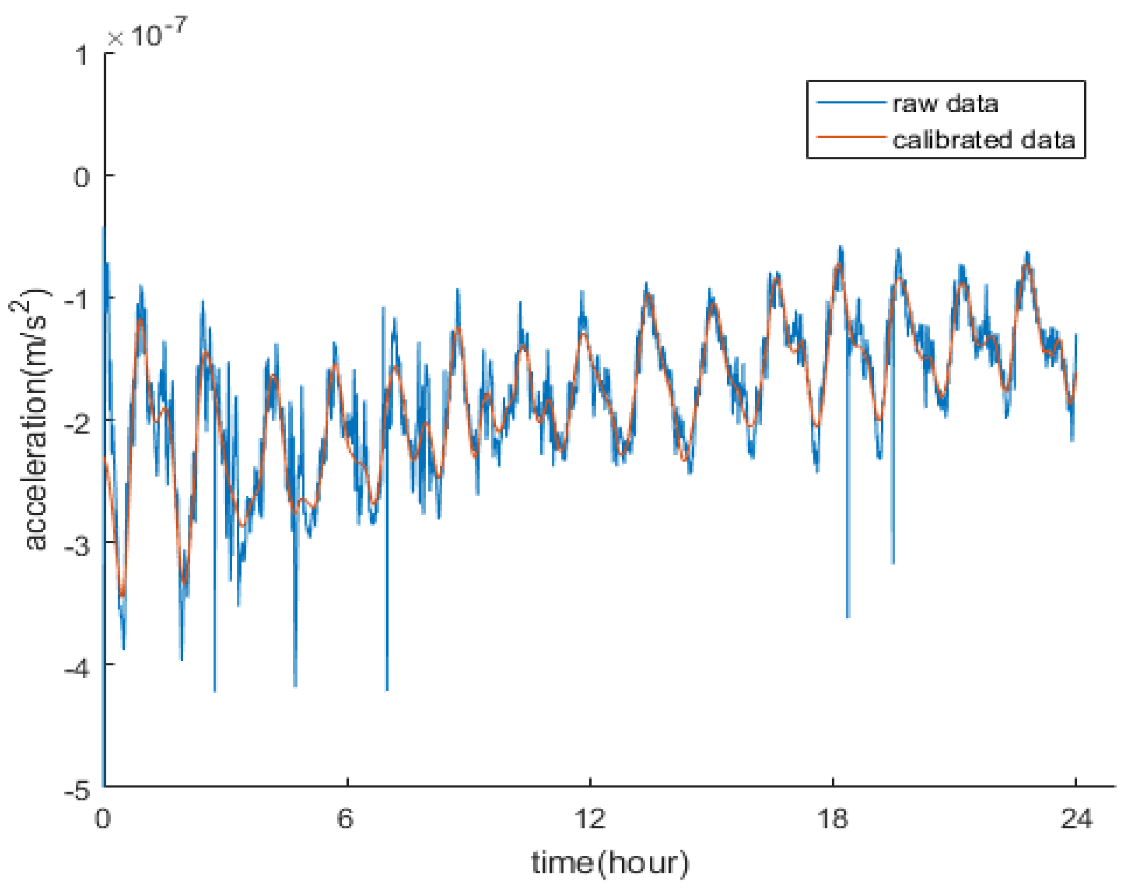
Abstract
:1. Introduction
- (1)
- Verify the atmospheric density obtained by the Swarm-C accelerometer inversion and use the atmospheric density obtained by the two-line orbital element method to verify the accuracy of the accelerometer inversion result;
- (2)
- The accelerometer’s density result and result from the two-line orbital number inversion were compared to discuss the accelerometer inversion of atmospheric density;
- (3)
- The accelerometer inversion results were used to evaluate the NRLMSISE-00 and JB2008 empirical atmosphere models. The accuracy and real-time performance of the two empirical atmosphere models were compared.
2. Data Acquisition and Processing
3. Methods
3.1. Conversion of Orbital Coordinates and Time
3.2. Calculation of Satellite Anti-Ballistic Coefficient
4. Results
4.1. Verification of Accelerometer Results from Swarm-C Satellite Orbit Data Inversion
4.2. Swarm-C Accelerometer Inversion Result Evaluation Empirical Atmosphere Model
5. Discussion
- (1)
- The two-line orbital element method was proposed in the verification experiment of the Swarm-C TLE results and Swarm-C accelerometer results. However, neither this method nor the semi-major axis attenuation method takes the light radiation pressure disturbance term into account. This method is only suitable for space objects below 1000 km because the reverse resistance of the atmosphere mainly causes an object’s resistance with an orbit of less than 1000 km. Once the object’s orbit is higher than 1000 km, the proportion of the light radiation pressure in the satellite’s resistance will increase. The error of the average translation term in the two-row orbit element data set will become more significant, so this method’s atmospheric density will be inaccurate. The radiation pressure model must be introduced if this method is used at altitudes above 1000 km. Because this is not the primary method studied in this article, no more detailed research will be done. The two-line track element data set is designed to facilitate data communication in the early period when communication is underdeveloped. It was used more in the early 1950s and 1980s. Due to the lack of data, the two-line orbital element number is now used for anti-ballistic coefficient and atmospheric density verification. It is a reference for the atmospheric density results obtained by precision orbits or accelerometers. However, its accuracy cannot meet the requirements when performing precise quantitative calculations;
- (2)
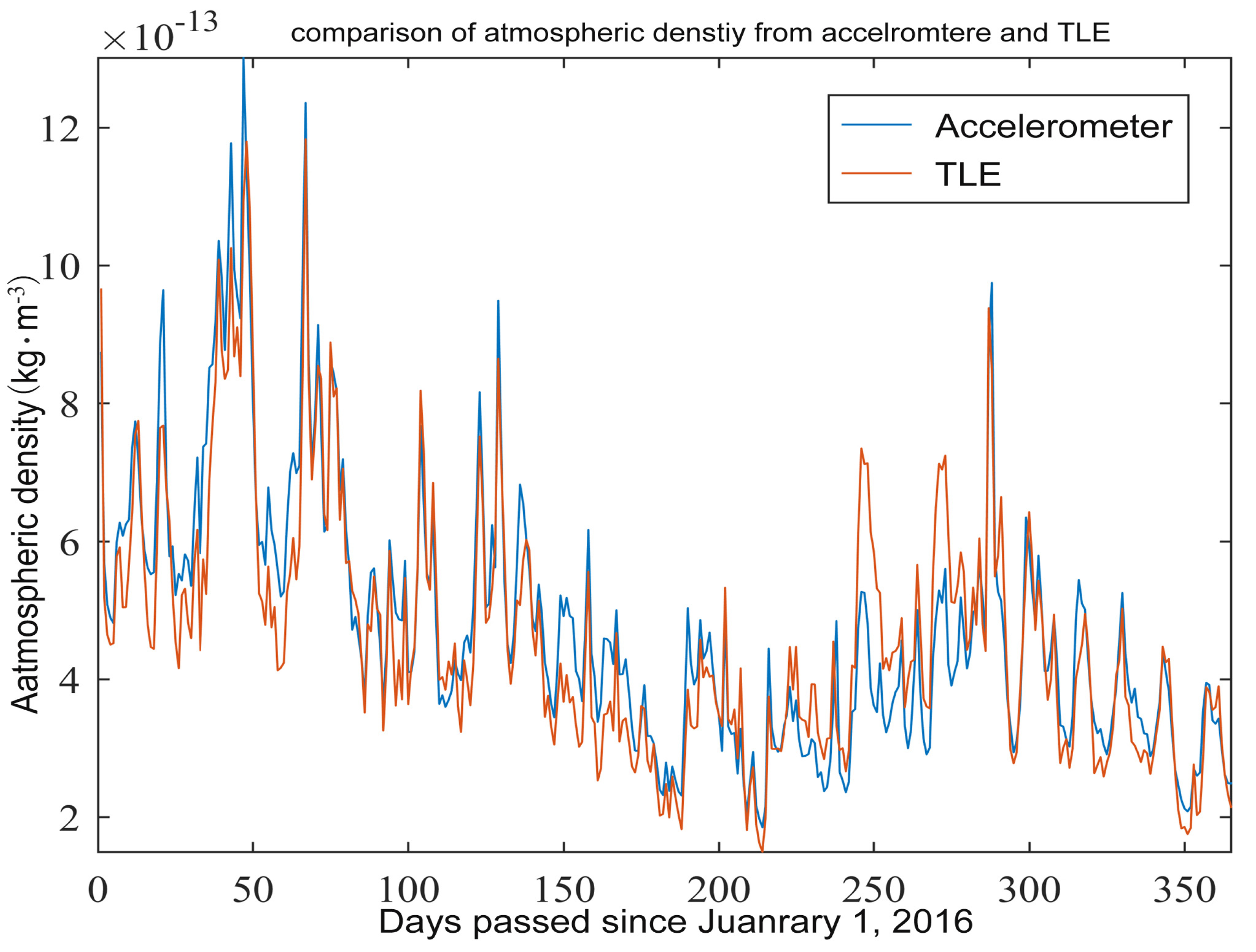
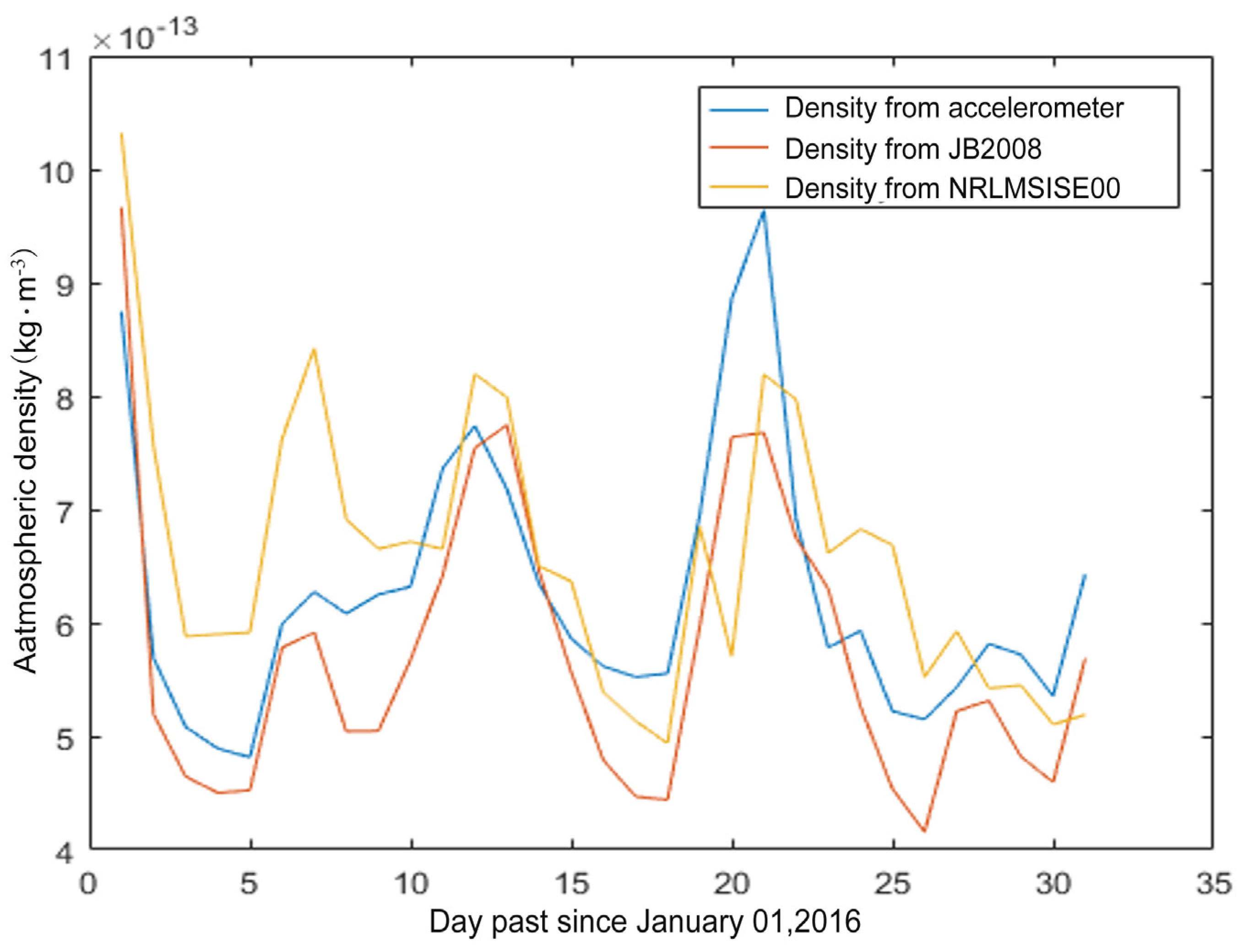
- In the Swarm-C accelerometer’s verification experiment using the results of the Swarm-C semi-major axis attenuation method, the use of the semi-major axis attenuation method requires high-precision HPOP orbit integration to obtain the average value of the semi-major axis changes in a minimal time range. The atmospheric density obtained by the semi-major axis attenuation method is the average atmospheric density during the integration time. Therefore, the semi-major axis attenuation method has low sensitivity and real-time performance compared with the accelerometer’s direct measurement of the atmospheric density. This feature can be seen in Figure 2. The semi-major axis attenuation method’s red density curve fluctuates much less than the accelerometer’s blue density curve. However, the real-time performance of the atmospheric density obtained by the semi-major axis attenuation method is not as good as that obtained by the accelerometer. Compared with the TLE method, the sampling frequency of the semi-major axis attenuation method satellite orbit data is much higher than the sampling frequency of the TLE two-line orbit element data. Although the semi-major axis attenuation method’s dynamics are not as good as the accelerometer’s atmospheric density, it is still better than the atmospheric density obtained by the two-line orbital element;
- (3)
- In the verification experiment of accelerometer results using the inversion results of Swarm-C orbit data, the results using accelerometer data are directly consistent with the results based on the semi-major axis change. It confirms the correction of the accelerometer calibration and the inversion of density. However, compared to the method that uses accelerometer data directly, the method based on the semi-major axis change is less dynamic. The use of accelerometers to extract atmospheric density has good real-time and dynamic properties. The extraction of atmospheric density using two-line orbital elements and atmospheric density extraction using the semi-major axis attenuation method are essentially the same. Both need to calculate the satellite’s semi-major axis change rate. Since the two-row orbit element data set does not contain satellite position parameters, calculating the atmospheric density by using the two-row orbit element number is necessary to calculate the satellite’s position and speed in the orbit parameters. However, because the two-row track element’s data sampling frequency is far lower than the accelerometer data sampling frequency, CelesTrak publishes only 1–2 sets of two-row orbit element data Swarm-C daily; the data that can be obtained is minimal. Therefore, the integration interval during orbital integration will be considerable. The integration interval selected here is 3 days, so the calculated satellite position and velocity errors are relatively large.Therefore, it can be found that the use of accelerometers to extract atmospheric density has better real-time and dynamic properties because the accelerometer measures instantaneous non-conservative force acceleration. However, this method requires accurate accelerometer calibration and accurate modeling of the light radiation pressure on the satellite surface. This study used the method to calibrate and correct the accelerometer. Since the deviation caused by other hardware issues is still not considered, errors will inevitably be introduced in the calibration process. It is also the primary source of the accelerometer’s error in extracting atmospheric density. Besides, there are errors caused by illumination radiation pressure modeling. However, this type of error is much smaller than the error introduced in the calibration process. Suppose ESA provides correction methods or corrected data. In that case, the accuracy of the atmospheric density extracted by the accelerometer will also be significantly improved;
- (4)
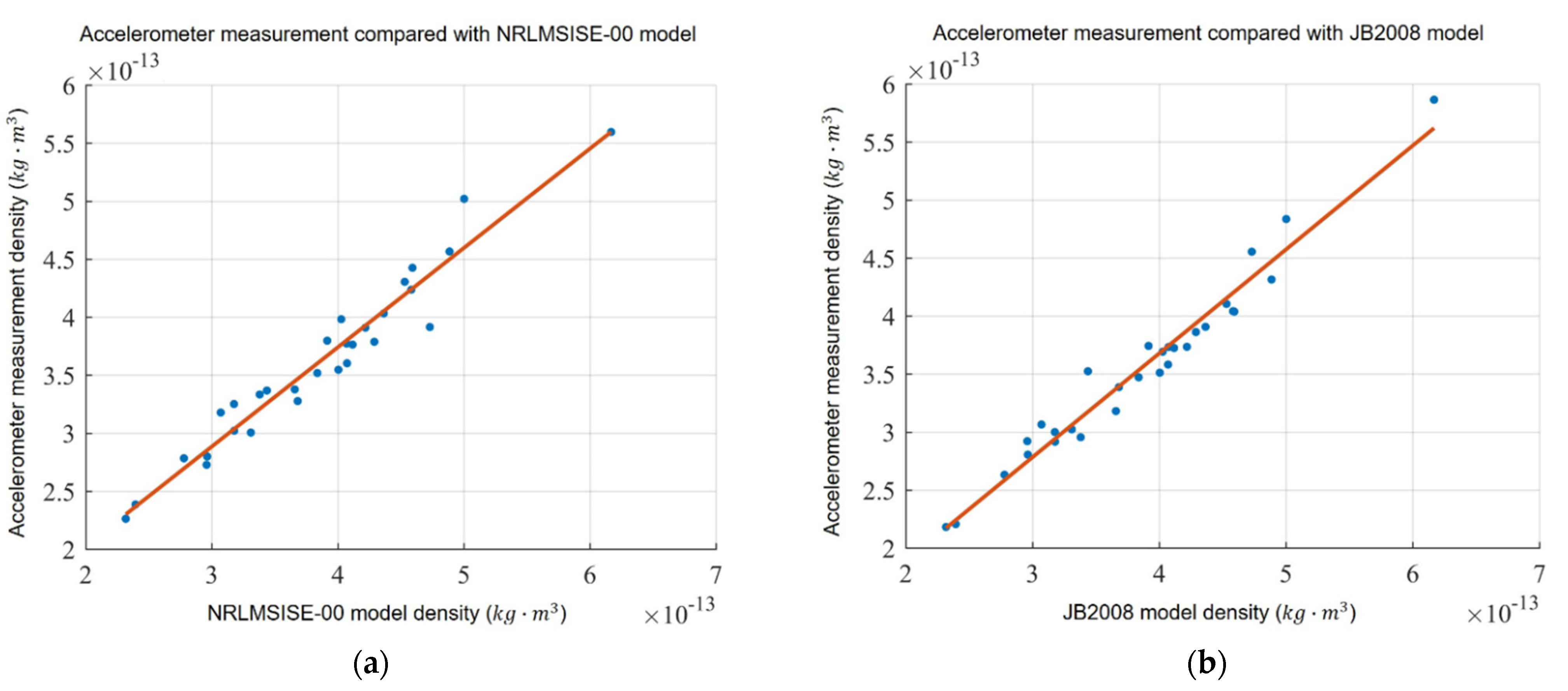
- In the experiment of evaluating the NRLMSISE-00 atmospheric model from the Swarm-C inversion results, Figure 5a shows a high degree of correlation between the atmospheric density obtained by using the accelerometer and the atmospheric density obtained by using the NRLMSISE-00 atmospheric density model. After calculation, the Pearson correlation coefficient of the two is 0.9528. According to general experience, if the Pearson coefficient is between 0.0–0.2, the two are irrelevant. Between 0.2–0.4, the two are weakly related. Between 0.4–0.6, the two are moderately correlated. Between 0.6–0.8, the two are strongly correlated. Between 0.8–1.0, the two are highly correlated. It shows that the atmospheric density obtained by the NRLMSISE-00 atmospheric model modeling and the accelerometer’s atmospheric density are already strongly correlated;
- (5)
- In the Swarm-C inversion results experiments to evaluate the JB2008 atmospheric model, Figure 5b shows the correlation degree of atmospheric density obtained using the accelerometer and JB2008 atmospheric density model higher than that of the accelerometer and NRLMSISE-00. After calculation, the Pearson correlation coefficient of the two has reached 0.9806. The Pearson correlation coefficient is more significant than 0.8, a robust correlation. It shows that the atmospheric density obtained by the JB2008 atmospheric model modeling and the accelerometer’s atmospheric density is strongly positively linear related;
- (6)
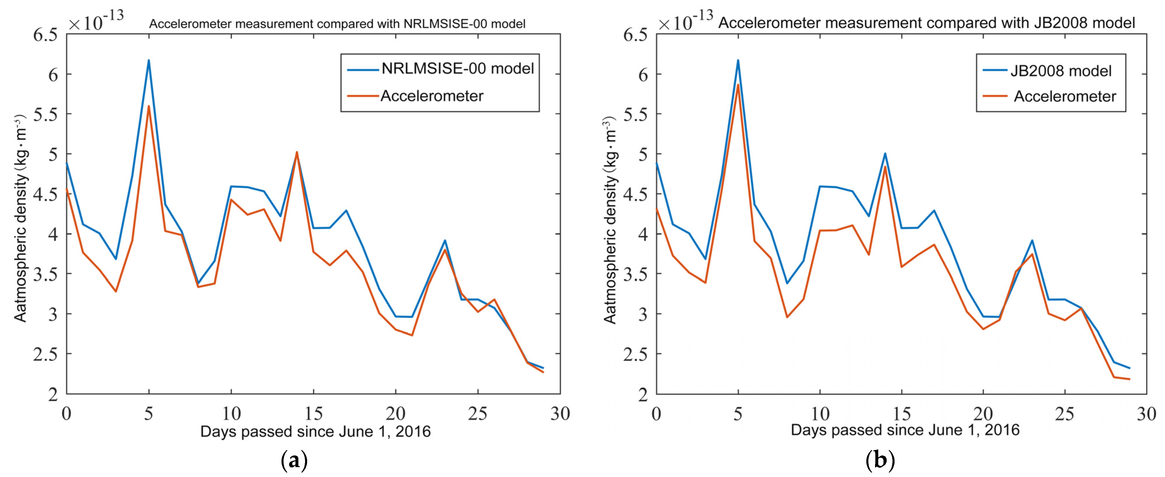
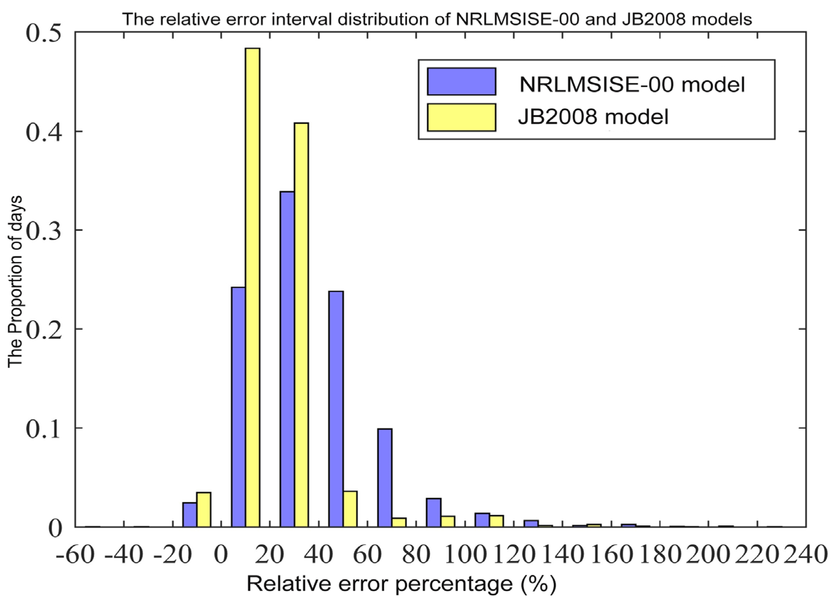
- In the experiment of evaluating the accuracy and real-time performance of the two atmospheric models, the JB2008 atmospheric model has a smaller delay and a faster response than the NRLMSISE-00 model. However, the NRLMSISE-00 model has also estimated some characteristics that the JB2008 model misses. On the whole, among the two peaks, the atmospheric density peak measured by the accelerometer is higher than the atmospheric density peak obtained by the two atmospheric models. Although the difference between the peak of the atmospheric model of NRLMSISE-00 and the accelerometer’s density is larger than that of JB2008, the NRLMSISE-00 has a better performance in estimating the overall pattern. Depending on the different expectations and usage, both models would have drawbacks and benefits. Moreover, the differences in performance accuracy are different in the two selected events. For example, the JB2008 model has a much better performance on 5 June than NRLMSISE-00, while 14 June is very similar. The model accuracy change may cause this phenomenon due to the solar cycle change. Depending on the different backgrounds and circumstances, the two models can be beneficial on different occasions. By understanding how the two model performance differs from different satellite data, the community would have a better understanding of how and what to use for their future studies;
- (7)
- From the experiment of using Swarm-C accelerometer inversion results to evaluate the empirical atmosphere model, it can be found that at the position where the Swarm-C satellite is flying, using the JB2008 atmospheric model for modeling will achieve better results than using the NRLMSISE-00 model, which means that the accuracy of the JB2008 atmospheric model at the altitude of the Swarn-C satellite is better than that of the NLRMSISE-00 atmospheric model. The altitude of Swarm-C satellite flight is about 500 km from the surface. It also verifies that the JB2008 atmospheric model proposed by Bruinsma et al. has a better simulation effect at altitudes below 500 km than the NRLMSISE-00 atmospheric model. The NRLMSISE-00 atmospheric model performs better than the JB2008 at altitudes above 500 km. This is because solar radiation has a heating effect on the atmosphere. The JB2008 atmospheric model considers the four bands of sunlight’s influence on the atmospheric density and corrects it. It also responds quickly to auroral heating. This is why the JB2008 atmospheric model has a better modeling effect here. It should be noted that the above discussion on the accuracy and real-time performance of the empirical atmosphere model is based on the geomagnetic calm period. However, the accuracy will change for periods of geomagnetic activity or magnetic storms. Therefore, the above results may not be valid [32].
6. Conclusions
Author Contributions
Funding
Institutional Review Board Statement
Informed Consent Statement
Data Availability Statement
Acknowledgments
Conflicts of Interest
References
- Emmert, J.T.; McDonald, S.E.; Drob, D.P.; Meier, R.R.; Lean, J.L.; Picone, J.M. Attribution of interminima changes in the global thermosphere and ionosphere. J. Geophys. Res. Space Phys. 2014, 119, 6657–6688. [Google Scholar] [CrossRef]
- Vickers, H.; Kosch, M.J.; Sutton, E.; Bjoland, L.; Ogawa, Y.; La Hoz, C. A solar cycle of upper thermosphere density observations from the EISCAT Svalbard Radar. J. Geophys. Res. Space Phys. 2014, 119, 6833–6845. [Google Scholar] [CrossRef] [Green Version]
- Zurek, R.W.; Tolson, R.A.; Bougher, S.W.; Lugo, R.A.; Baird, D.T.; Bell, J.M.; Jakosky, B.M. Mars thermosphere as seen in MAVEN accelerometer data. J. Geophys. Res. Space Phys. 2017, 122, 3798–3814. [Google Scholar] [CrossRef]
- Drob, D.; Emmert, J.; Crowley, G.; Picone, J.; Shepherd, G.; Skinner, W.; Hays, P.; Niciejewski, R.; Larsen, M.; She, C. An empirical model of the Earth’s horizontal wind fields: HWM07. J. Geophys. Res. Space Phys. 2008, 113, A12. [Google Scholar] [CrossRef]
- Grivas, G.; Chaloulakou, A. Artificial neural network models for prediction of PM10 hourly concentrations, in the Greater Area of Athens, Greece. Atmos. Environ. 2006, 40, 1216–1229. [Google Scholar] [CrossRef]
- Holben, B.N.; Eck, T.F.; Slutsker, I.; Tanré, D.; Buis, J.P.; Setzer, A.; Vermote, E.; Reagan, J.A.; Kaufman, Y.J.; Nakajima, T.; et al. AERONET—A Federated Instrument Network and Data Archive for Aerosol Characterization. Remote Sens. Environ. 1998, 66, 1–16. [Google Scholar] [CrossRef]
- Slini, T.; Kaprara, A.; Karatzas, K.; Moussiopoulos, N. PM10 forecasting for Thessaloniki, Greece. Environ. Model. Softw. 2006, 21, 559–565. [Google Scholar] [CrossRef]
- Liu, H.; Hirano, T.; Watanabe, S. Empirical model of the thermospheric mass density based on CHAMP satellite observations. J. Geophys. Res. Space Phys. 2013, 118, 843–848. [Google Scholar] [CrossRef]
- Bowman, B.; Tobiska, W.K.; Marcos, F.; Huang, C.; Lin, C.; Burke, W. A New Empirical Thermospheric Density Model JB2008 Using New Solar and Geomagnetic Indices. In Proceedings of the AIAA/AAS Astrodynamics Specialist Conference and Exhibit, Honolulu, HI, USA, 18–21 August 2008; p. 6438. [Google Scholar] [CrossRef] [Green Version]
- Doornbos, E. Thermospheric Density and Wind Determination from Satellite Dynamics; Springer Science & Business Media: Berlin/Heidelberg, Germany, 2012. [Google Scholar]
- Picone, J.M.; Hedin, A.E.; Drob, D.P.; Aikin, A.C. NRLMSISE-00 empirical model of the atmosphere: Statistical comparisons and scientific issues. J. Geophys. Res. 2002, 107, 1468. [Google Scholar] [CrossRef]
- Seo, S.; Kim, J.; Lee, H.; Jeong, U.; Kim, W.; Holben, B.N.; Kim, S.-W.; Song, C.H.; Lim, J.H. Estimation of PM10 concentrations over Seoul using multiple empirical models with AERONET and MODIS data collected during the DRAGON-Asia campaign. Atmos. Chem. Phys. 2015, 15, 319–334. [Google Scholar] [CrossRef] [Green Version]
- Zheng, W.; Li, X.; Xie, J.; Yin, L.; Wang, Y. Impact of human activities on haze in Beijing based on grey relational analysis. Rend. Lince 2015, 26, 187–192. [Google Scholar] [CrossRef]
- Rajendra, P.P.; Kuga, H.K. An evaluation of Jacchia and MSIS 90 atmospheric models with CBERS data. Acta Astronaut. 2001, 48, 579–588. [Google Scholar] [CrossRef]
- Xu, J.; Wang, W.; Zhang, S.; Liu, X.; Yuan, W. Multiday thermospheric density oscillations associated with variations in solar radiation and geomagnetic activity. J. Geophys. Res. Space Phys. 2015, 120, 3829–3846. [Google Scholar] [CrossRef]
- Murray, S.A.; Henley, E.M.; Jackson, D.R.; Bruinsma, S.L. Assessing the performance of thermospheric modeling with data assimilation throughout solar cycles 23 and 24. Space Weather 2015, 13, 220–232. [Google Scholar] [CrossRef] [Green Version]
- Shim, J.; Kuznetsova, M.; Rastätter, L.; Bilitza, D.; Butala, M.; Codrescu, M.; Emery, B.; Foster, B.; Fuller-Rowell, T.; Huba, J. CEDAR Electrodynamics Thermosphere Ionosphere (ETI) Challenge for systematic assessment of ionosphere/thermosphere models: Electron density, neutral density, NmF2, and hmF2 using space based observations. Space Weather 2012, 10, 10. [Google Scholar] [CrossRef] [Green Version]
- Bezdek, A. Calibration of accelerometers aboard GRACE satellites by comparison with POD-based nongravitational accelerations. J. Geodyn. 2010, 50, 410–423. [Google Scholar] [CrossRef] [Green Version]
- Liu, S.; Gao, Y.; Zheng, W.; Li, X. Performance of two neural network models in bathymetry. Remote Sens. Lett. 2015, 6, 321–330. [Google Scholar] [CrossRef]
- Reid, C.E.; Jerrett, M.; Petersen, M.L.; Pfister, G.G.; Morefield, P.E.; Tager, I.B.; Raffuse, S.M.; Balmes, J.R. Spatiotemporal Prediction of Fine Particulate Matter During the 2008 Northern California Wildfires Using Machine Learning. Environ. Sci. Technol. 2015, 49, 3887–3896. [Google Scholar] [CrossRef]
- Picone, J.M.; Emmert, J.T.; Lean, J. Thermospheric densities derived from spacecraft orbits: Accurate processing of two-line element sets. J. Geophys. Res. Earth Surf. 2005, 110. [Google Scholar] [CrossRef]
- Siemes, C.; Da Encarnação, J.D.T.; Doornbos, E.; Van Den Ijssel, J.; Kraus, J.; Pereštý, R.; Grunwaldt, L.; Apelbaum, G.; Flury, J.; Olsen, P.E.H. Swarm accelerometer data processing from raw accelerations to thermospheric neutral densities. Earth Planets Space 2016, 68, 1–16. [Google Scholar] [CrossRef] [Green Version]
- Ijssel, J.V.D.; Doornbos, E.; Iorfida, E.; March, G.; Siemes, C.; Montenbruck, O. Thermosphere densities derived from Swarm GPS observations. Adv. Space Res. 2020, 65, 1758–1771. [Google Scholar] [CrossRef]
- Bezděk, A.; Sebera, J.; Klokočník, J. Calibration of Swarm accelerometer data by GPS positioning and linear temperature correction. Adv. Space Res. 2018, 62, 317–325. [Google Scholar] [CrossRef]
- Mehta, P.M.; Walker, A.C.; Sutton, E.K.; Godinez, H.C. New density estimates derived using accelerometers on board the CHAMP and GRACE satellites. Space Weather 2017, 15, 558–576. [Google Scholar] [CrossRef]
- Weimer, D.; Mlynczak, M.; Emmert, J.; Doornbos, E.; Sutton, E.; Hunt, L. Correlations between the thermosphere’s semiannual density variations and infrared emissions measured with the SABER instrument. J. Geophys. Res. Space Phys. 2018, 123, 8850–8864. [Google Scholar] [CrossRef] [Green Version]
- March, G.; Doornbos, E.; Visser, P. High-fidelity geometry models for improving the consistency of CHAMP, GRACE, GOCE and Swarm thermospheric density data sets. Adv. Space Res. 2018, 63, 213–238. [Google Scholar] [CrossRef]
- Sentman, L.H. Free Molecule Flow Theory and Its Application to the Determination of Aerodynamic Forces; Lockheed Missiles and Space Co. Inc.: Sunnyvale, CA, USA, 1961. [Google Scholar]
- Kodikara, T.; Carter, B.; Zhang, K. The First Comparison Between Swarm-C Accelerometer-Derived Thermospheric Densities and Physical and Empirical Model Estimates. J. Geophys. Res. Space Phys. 2018, 123, 5068–5086. [Google Scholar] [CrossRef]
- Qian, L.; Solomon, S. Thermospheric Density: An Overview of Temporal and Spatial Variations. Space Sci. Rev. 2011, 168, 147–173. [Google Scholar] [CrossRef]
- Zhou, Y.; Zheng, W.; Shen, Z. A New Algorithm for Distributed Control Problem with Shortest-Distance Constraints. Math. Probl. Eng. 2016, 2016, 1–6. [Google Scholar] [CrossRef]
- Calabia, A.; Jin, S. Thermospheric density estimation and responses to the March 2013 geomagnetic storm from GRACE GPS-determined precise orbits. J. Atmos. Solar-Terr. Phys. 2017, 154, 167–179. [Google Scholar] [CrossRef]


Publisher’s Note: MDPI stays neutral with regard to jurisdictional claims in published maps and institutional affiliations. |
© 2022 by the authors. Licensee MDPI, Basel, Switzerland. This article is an open access article distributed under the terms and conditions of the Creative Commons Attribution (CC BY) license (https://creativecommons.org/licenses/by/4.0/).
Share and Cite
Yin, L.; Wang, L.; Zheng, W.; Ge, L.; Tian, J.; Liu, Y.; Yang, B.; Liu, S. Evaluation of Empirical Atmospheric Models Using Swarm-C Satellite Data. Atmosphere 2022, 13, 294. https://doi.org/10.3390/atmos13020294
Yin L, Wang L, Zheng W, Ge L, Tian J, Liu Y, Yang B, Liu S. Evaluation of Empirical Atmospheric Models Using Swarm-C Satellite Data. Atmosphere. 2022; 13(2):294. https://doi.org/10.3390/atmos13020294
Chicago/Turabian StyleYin, Lirong, Lei Wang, Wenfeng Zheng, Lijun Ge, Jiawei Tian, Yan Liu, Bo Yang, and Shan Liu. 2022. "Evaluation of Empirical Atmospheric Models Using Swarm-C Satellite Data" Atmosphere 13, no. 2: 294. https://doi.org/10.3390/atmos13020294