Evaluation of the Homogenization Adjustments Applied to European Temperature Records in the Global Historical Climatology Network Dataset

Abstract

The widely used Global Historical Climatology Network (GHCN) monthly temperature dataset is available in two formats—non-homogenized and homogenized. Since 2011, this homogenized dataset has been updated almost daily by applying the “Pairwise Homogenization Algorithm” (PHA) to the non-homogenized datasets. Previous studies found that the PHA can perform well at correcting synthetic time series when certain artificial biases are introduced. However, its performance with real world data has been less well studied. Therefore, the homogenized GHCN datasets (Version 3 and 4) were downloaded almost daily over a 10-year period (2011–2021) yielding 3689 different updates to the datasets. The different breakpoints identified were analyzed for a set of stations from 24 European countries for which station history metadata were available. A remarkable inconsistency in the identified breakpoints (and hence adjustments applied) was revealed. Of the adjustments applied for GHCN Version 4, 64% (61% for Version 3) were identified on less than 25% of runs, while only 16% of the adjustments (21% for Version 3) were identified consistently for more than 75% of the runs. The consistency of PHA adjustments improved when the breakpoints corresponded to documented station history metadata events. However, only 19% of the breakpoints (18% for Version 3) were associated with a documented event within 1 year, and 67% (69% for Version 3) were not associated with any documented event. Therefore, while the PHA remains a useful tool in the community’s homogenization toolbox, many of the PHA adjustments applied to the homogenized GHCN dataset may have been spurious. Using station metadata to assess the reliability of PHA adjustments might potentially help to identify some of these spurious adjustments.

1. Introduction

The National Oceanic and Atmospheric Administration (NOAA)’s National Centers for Environmental Information (NCEI) provide one of the most widely used monthly land surface temperature datasets, the Global Historical Climatology Network (GHCN) [1,2,3,4]. As can be seen from

Table 1. Usage of the Global Historical Climatology Network (GHCN) dataset by current global and hemispheric land surface temperature estimates. Each of the listed temperature time series uses either the unhomogenized (“raw”) or homogenized GHCN dataset as either the primary (1°) or a secondary (2°) data source. If additional homogenization steps are applied to these GHCN station records before use, this is noted in the right-hand column.

Time Series	GHCN (Raw)	GHCN (Homogenized)	Extra Homogenization
NOAA National Centers for Environmental Information (NCEI), “NOAAGlobalTemp” [3,4,5,6]	×	1° data source	No
NASA Goddard Institute for Space Studies (GISS), “GISTEMP” [7,8]	×	1° data source	Yes
Japan Meteorological Agency (JMA) [9]	×	1° data source	No
Climate Research Unit (CRU), “CRUTEM” [10,11]	×	1° source for U.S.; 2° source for rest of world	No
Chinese Meteorological Administration (CMA), “C-LSAT” [12,13,14]	2° source for global data	1° source for U.S.	Yes, except for U.S. component
Berkeley Earth, “BEST” [15,16,17]	2° data source	×	Yes
Connolly et al. (2021), “Rural-only Northern Hemisphere” [18,19]	1° data source	×	Yes

, it is either the primary (1°) or a major secondary (2°) instrumental data source for each of the current global and hemispheric land surface temperature estimates [3,4,5,6,7,8,9,10,11,12,13,14,15,16,17,18,19].

The first version of the dataset (released in 1992 by NOAA’s National Climatic Data Center—which became NCEI in 2015) did not attempt to correct for non-climatic biases in the station records [1]. However, starting with Version 2 (released in 1997), NOAA have provided two alternate variants of the dataset [2]. The first variant contains the original (henceforth, “raw” or “unhomogenized”) temperature records without any attempt to correct for non-climatic biases. For the other variant (henceforth, “homogenized”), all station records are processed using an automated statistical homogenization program.

Since Version 2, the GHCN includes a separately processed dataset for the contiguous United States (i.e., all states except Alaska and Hawai’i) called the United States Historical Climatology Network (USHCN) [20,21]. This is a high-density network of relatively long station records (~1200 stations, spanning the period 1895–present) for which NOAA maintains detailed “station history metadata”, i.e., records describing details and dates of any documented changes in the types of thermometer used, observation practices, station location, etc. As we will discuss later, access to such station history metadata can potentially be very useful for identifying and correcting for non-climatic biases in the station records. However, for the rest of the GHCN stations, NOAA did not acquire any of this station history metadata. Instead, the station metadata for the rest of the GHCN stations are limited to “station environment metadata”, i.e., details on the most recent station location, e.g., current station name, latitude, longitude and elevation [2,3,4]. Given this extra information for the contiguous U.S. component, NOAA processes and homogenizes the USHCN dataset separately from the rest of the GHCN dataset and merges the two components later [2,3,4].

For Version 2 of the GHCN, NOAA applied very different homogenization techniques to both components. The USHCN component was homogenized using the station history metadata to correct for changes in “time of observation” (TOB) [22] and changes in instrumentation [23] using empirically-derived corrections. Non-climatic biases arising from other documented changes were estimated using the relative homogeneity adjustment algorithm of Karl & Williams (1987) [24]. A separate population-based correction for potential urbanization bias was also applied [25] along with some infilling of data gaps [20]. In contrast, for the rest of the GHCN, NOAA applied the Easterling and Peterson (1995) [26] relative homogeneity adjustment algorithm. This algorithm was designed to statistically identify both the date and magnitude of any non-climatic jumps (“breakpoints”) in the station record relative to a reference time series constructed from the average of five neighboring stations [2,26]. As a result, it does not require or use any station metadata other than latitude and longitude.

In 2009, NOAA developed Version 2 of the USHCN [21] which replaced the previous explicit corrections for changes in instrumentation and urbanization bias as well as the Karl & Williams (1987) homogenization algorithm with the new Pairwise Homogeneity Adjustment (PHA) algorithm described by Menne & Williams (2009) [27]. This PHA algorithm was designed to identify non-climatic breakpoints that were either documented (i.e., associated with a known station history metadata event) or undocumented. The algorithm requires less strict statistical thresholds for potential breakpoints occurring shortly before or after a documented metadata event. Menne & Williams (2009) showed that the algorithm fared quite well when applied to synthetic time series where artificial biases had been intentionally added [27]. Menne et al. (2009) later argued that the PHA coincidentally also indirectly removed much of the urbanization biases in station records—citing the PHA results for one station (Reno, Nevada, USA) as an example [21]. Therefore, for USHCN version 2, the previous explicit corrections for urbanization bias and changes in instrumentation were dropped. Instead, it was argued that the PHA adjustments for both documented and undocumented events should be adequate for correcting all of these non-climatic biases [21], although the TOB adjustments were kept as-is, on the basis of Vose et al. (2003)’s analysis [28]. Later, Menne et al. (2010) [29] argued that the PHA adjustments were also indirectly capable of identifying and removing non-climatic biases arising from degradations over time in the quality of the exposure of many USHCN stations [30,31,32,33] that had been revealed to be widespread and systemic by the voluntary citizen science “Surfacestations” project [33].

Therefore, when NOAA introduced Version 3 of the GHCN in 2011, they decided to switch to also using the PHA for homogenizing the non-USHCN component [3]. This decision was repeated for the current Version 4 that was introduced as a “beta” version in 2015, and formally launched in 2018 [4].

NOAA still has not collected station history metadata for analyzing any of the GHCN stations (other than the USHCN component). Therefore, the PHA is applied to the non-USHCN component of the GHCN in “undocumented events only” mode. However, several “benchmarking” evaluations have found that the PHA performs quite well at correcting synthetic time series “blind” when certain artificial biases are introduced [34,35,36], i.e., when run in “undocumented events only” mode. Moreover, as mentioned above, Menne et al. have argued that the PHA is indirectly quite successful at correcting for long-term non-climatic biases from urbanization [29] and reductions in the quality of station exposure [29]. Hausfather et al. (2013) support this claim [37].

On the other hand, Soon et al. argue that much of the apparent “removal” of urbanization biases and poor station exposure biases via homogenization is a statistical artefact of the homogenization process which leads to the “blending” of non-climatic biases [18,19,38,39]. That is, if several of the reference neighboring stations are affected by gradual multidecadal biases such as urbanization bias then, when the sign and magnitude of a given breakpoint is being calculated by the homogenization algorithm, some of these biases may inadvertently be added to the homogenized record. This “aliasing” of biases has now been demonstrated as a systemic statistical artefact of standard homogenization algorithms by several studies [32,38,40].

As a result, the more breakpoints are adjusted for each record, the more the trends of that record will tend to converge towards the trends of its neighbors. Initially, this might appear desirable since the trends of the homogenized records will be more homogeneous (arguably one of the main goals of “homogenization”), and therefore some have objected to this criticism [41]. However, if multiple neighbors are systemically affected by similar long-term non-climatic biases, then the homogenized trends will tend to converge towards the averages of the station network (including systemic biases), rather than towards the true climatic trends of the region.

Soon et al. (2018) suggest that one way to minimize this blending problem of homogenization would be to ensure that the neighbor network used for the homogenization process is not systemically biased relative to the target stations, e.g., rural stations should be homogenized using a mostly rural station network [38]. Indeed, they note that Ren et al. have effectively carried this out for their homogenization of Chinese records for the post-1960 period [42,43]. However, this is a non-trivial challenge for future research, which is beyond the scope of this paper.

At any rate, in Soon et al. (2015), three of us noted an additional concern over the PHA adjustments applied by NOAA to the GHCN dataset [18]. While evaluating rural temperature trends for Ireland, Soon et al. (2015) noted several oddities with the homogenized GHCN record (then Version 3) for the longest rural Irish record in the dataset, i.e., Valentia Observatory [18]:

• There was a concerning lack of consistency in the breakpoints and adjustments applied by NOAA to the record between each of the five different updates of the GHCN dataset the authors had downloaded (October 2011, January 2012, January 2013, July 2014 and January 2015);
• None of the breakpoints identified by NOAA’s PHA for any of those updates corresponded to any of the four documented events in the station history metadata which the Valentia Observatory observers provided;
• The PHA homogenization failed to identify, in any of those updates, non-climatic biases associated with the major station move in 1892 or the second station move in 2001 for which parallel measurements showed a −0.3 °C cooling bias.

Independently, another one of us (P.O’N.) had been regularly downloading and archiving the updates of the datasets for research purposes from NOAA’s website since May 2011—initially roughly fortnightly, but later updated to roughly weekly (March 2012) and eventually (March 2014) daily using an automated script. By early 2015, he had also begun noticing the remarkable lack of consistency in PHA adjustments between different updates of the GHCN dataset. Therefore, he continued archiving NOAA’s roughly daily updates to the dataset. This extensive archive of NOAA’s updates to the GHCN dataset is the main basis for the analysis in this paper. This comprises 1877 updates of Version 3 and 1812 updates of Version 4.

Meanwhile, Soon et al. (2015) had fortuitously been able to directly ground-truth the various adjustments to the Valentia Observatory record because the station observers had provided access to both the station history metadata and accompanying parallel measurements for two of the more recent events [18]. However, at the time, access to publicly archived station history metadata for other stations was extremely limited.

Still, over the last decade or so, particularly in Europe, there has been an increasing realization of the importance of not only tracking down and digitizing early historical weather records [44,45,46,47,48,49,50,51,52,53], but also identifying and digitizing the relevant station history metadata associated with temperature records [46,47,48,49,50,51,52,53,54,55,56,57,58]. Therefore, for quite a few of the GHCN stations, relevant history metadata are now available.

Some of these station history metadata have been published in the scientific literature, e.g., [52,54,58,59,60,61,62,63,64,65], while others are archived by various organizations such as national meteorological services, e.g., [51,66,67,68]. However, much of the collected station metadata are part of ongoing digitizing projects, e.g., [46,47,48,49,50,55,56,57,69,70,71], and are not yet publicly archived. In addition, analyzing and interpreting the relevance of historical metadata for evaluating homogenization adjustments can be somewhat subjective. Therefore, for this collaborative study, the first four listed co-authors sought the assistance of the remaining co-authors in compiling and analyzing the station history metadata from as many GHCN stations as possible for the European region. At the time of writing, we have compiled relevant station history metadata for more than 800 European GHCN stations, and these stations will be the basis for this analysis.

In this paper, we will use this unique combination of the extensive archive of more than 1,800 iterations each of Version 3 and 4 of the GHCN datasets along with our compilation of station history metadata to quantify and evaluate the PHA adjustments that have been applied by NOAA to the GHCN dataset since 2011 [3,4]. We appreciate that the PHA [27] has performed quite well over the years in various studies, including benchmarking tests [27,34,35,36]. However, these earlier assessments of the PHA were generally “one-off” assessments, i.e., they did not evaluate the consistency of the breakpoints and adjustments applied with repeated runs of the algorithm.

Nominally, our analysis in this study is confined to Europe, since this is the region for which we have compiled the relevant station history metadata. However, this region comprises many of the longest and most complete station records in the GHCN dataset, and we therefore think the results from this case study are of relevance to all users of the GHCN dataset. We also expect our findings will be of interest to the temperature homogenization community.

The main aims of this study are:

• To describe how the PHA adjustments applied to the stations in the widely-used GHCN datasets vary between updates, using this subset of European stations as a detailed case study for the entire global dataset.
• To evaluate how closely related (or otherwise) the breakpoints identified by the PHA process are to documented station history metadata events.
• To discuss the implications these findings have for the scientific community’s goals of accurately estimating regional climatic temperature trends.
• To make recommendations for steps the temperature homogenization community can take to resolve some of the identified problems, moving forward.

2. Materials and Methods

2.1. Timeline of How Our Archive of GHCN Datasets Was Compiled

NOAA NCEI update the GHCN-monthly datasets and rerun the PHA homogenization program approximately daily and upload it to their website (currently https://www.ncei.noaa.gov/products/land-based-station/global-historical-climatology-network-monthly [accessed on 24 December 2021]).

As discussed above, each time the PHA program is run, the homogenized GHCN dataset generated is different from the previous iteration. Initially, we might expect the adjustments applied to each station record to remain fairly consistent from run to run.

For instance, we might expect the adjustments to vary occasionally as each of the still-active stations’ records are updated with the latest month’s data. Also, as the dataset is updated, the “40 out of 100 nearest neighbors” used by the PHA for homogenizing an individual station could change from run to run [27]. However, as we will discuss in detail later, the adjustments applied to each station record will often change quite dramatically between runs as NOAA updates the dataset and re-runs their homogenization program. Each run will often identify new breakpoints throughout the entire record and often will drop breakpoints which had been identified on previous runs.

As a result, the homogenized temperatures for any given station in, e.g., the mid-19th century might be very different in Tuesday’s dataset than they were in Monday’s dataset, for instance. For other stations, the homogenized records might remain essentially the same every time the homogenization program is run over the years.

Fortunately, as mentioned in the introduction, one of us (P.O’N.) began regularly downloading and archiving the latest versions of the GHCN datasets from NOAA’s website in 2011—initially roughly fortnightly, but daily since March 2014.

Table 2. Numbers of distinct GHCN datasets downloaded from NOAA’s website for each year. Version 4 was originally introduced as a “beta” version in October 2015 until the official version was released in October 2018. Version 3 was discontinued in August 2019. For this study, we consider all distinct datasets up to July/August 2021 (some stations were analyzed up to July and others up to August). This comprises 1877 for version 3 (covering the period 2011–2019) and 1812 for version 4 (covering the period 2015–2021).

Year	GHCN Version 3	GHCN Version 4	Version 4 (“Beta”)
2011	6	-	-
2012	39	-	-
2013	34	-	-
2014	283	-	-
2015	316	71	(71)
2016	342	303	(303)
2017	346	322	(322)
2018	315	314	(256)
2019	196	287	-
2020	-	310	-
2021	-	205	-
Total distinct datasets	1877	1812	(952)

shows the number of different iterations of the datasets in his archive that were downloaded for each year. The timeline of how frequently the datasets have been downloaded is described below:

• May 2011: P.O’N. began downloading and archiving the dataset (then version 3) from NOAA’s website roughly fortnightly.
• March 2012: The download rate was increased to roughly weekly.
• March 2014: An automated script was set up to download the dataset daily. However, NOAA’s updates appear to have been only approximately every 24 hours. Therefore, on some days, the datasets downloaded were identical to the preceding day. We have removed these identical copies from our analysis. Furthermore, on some days, the download was not carried out due to P.O’N’s computer being offline for maintenance or travel. Hence, the annual totals for each dataset in Table 2 are less than 365 for all years.
• October 2015: NOAA launched the “beta” version 4. Therefore, P.O’N. began downloading and archiving both version 3 and 4 daily.
• October 2018: NOAA launched the official version 4. For the purposes of this analysis, we have treated the “beta” and official version 4 datasets as equivalent, but for reference we have listed the numbers of “beta” datasets downloaded in the right-hand column of Table 2.
• August 2019: NOAA discontinued version 3.
• July to August 2021: P.O’N. processed the data for each of the stations in this analysis in several stages over the period from 7 July–20 August 2021. However, he still continues to download and archive the dataset daily at the time of writing.

2.2. Station History Metadata Available

Figure 1 shows the locations of all the European GHCN stations for which we compiled station history metadata (filled red circles) as well as the remaining stations for which we had not yet identified station history metadata at the time of writing.

Table 3. Numbers of Global Historical Climatology Network (GHCN) stations for each country analyzed for this study. The stations analyzed were those for which we have obtained station history metadata.

	GHCN v3			GHCN v4
Country	With Metadata	No Metadata	Analyzed	With Metadata	No Metadata	Analyzed
Austria	11	2	85%	53	11	83%
Belgium	1	0	100%	1	19	5%
Bulgaria	11	0	100%	32	2	94%
Croatia	13	0	100%	19	2	90%
Czech Republic	4	11	27%	23	18	56%
Denmark	4	6	40%	16	13	55%
Estonia	2	3	40%	3	20	13%
Finland	2	16	11%	3	329	1%
France	23	20	53%	106	18	85%
Germany	23	57	29%	77	697	10%
Greece	15	0	100%	40	0	100%
Hungary	7	1	88%	26	1	96%
Ireland	15	0	100%	30	1	97%
Italy	5	95	5%	5	200	2%
The Netherlands	2	0	100%	37	15	71%
Norway	19	14	58%	127	275	32%
Poland	52	9	85%	60	10	86%
Russia (“European”)	1	65	2%	2	272	1%
Slovakia	8	0	100%	20	0	100%
Spain	1	34	3%	2	135	1%
Sweden	3	16	16%	5	645	1%
Switzerland	10	1	91%	37	7	84%
Ukraine	25	2	93%	119	3	98%
United Kingdom	2	56	3%	4	182	2%
24 countries	259	408	39%	847	2875	23%

lists the total station counts for each country. Details on the sources for these station history metadata are provided in the Supplementary Materials.

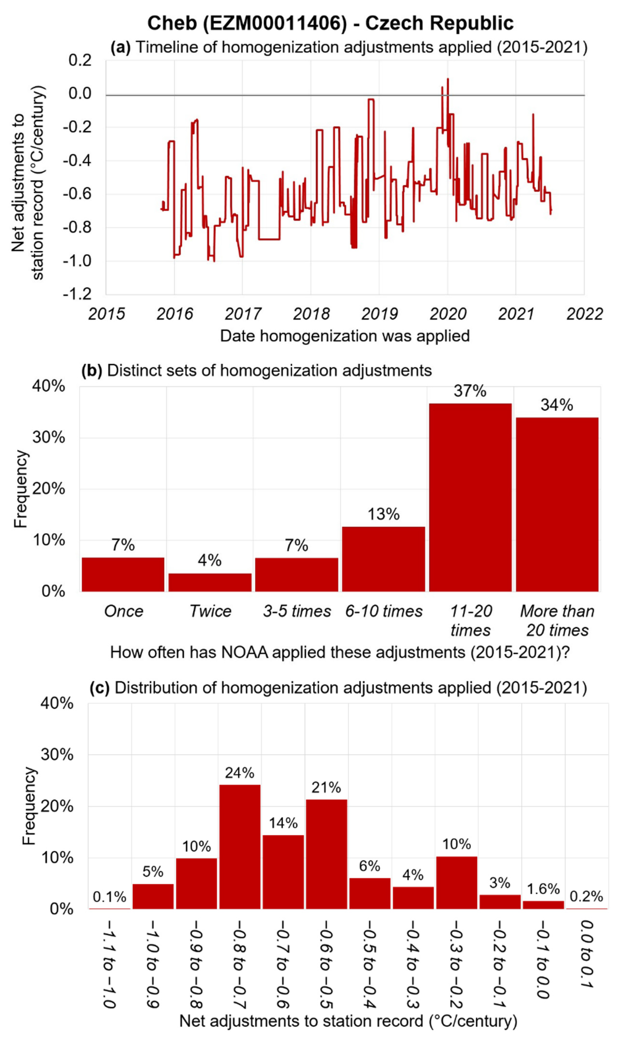
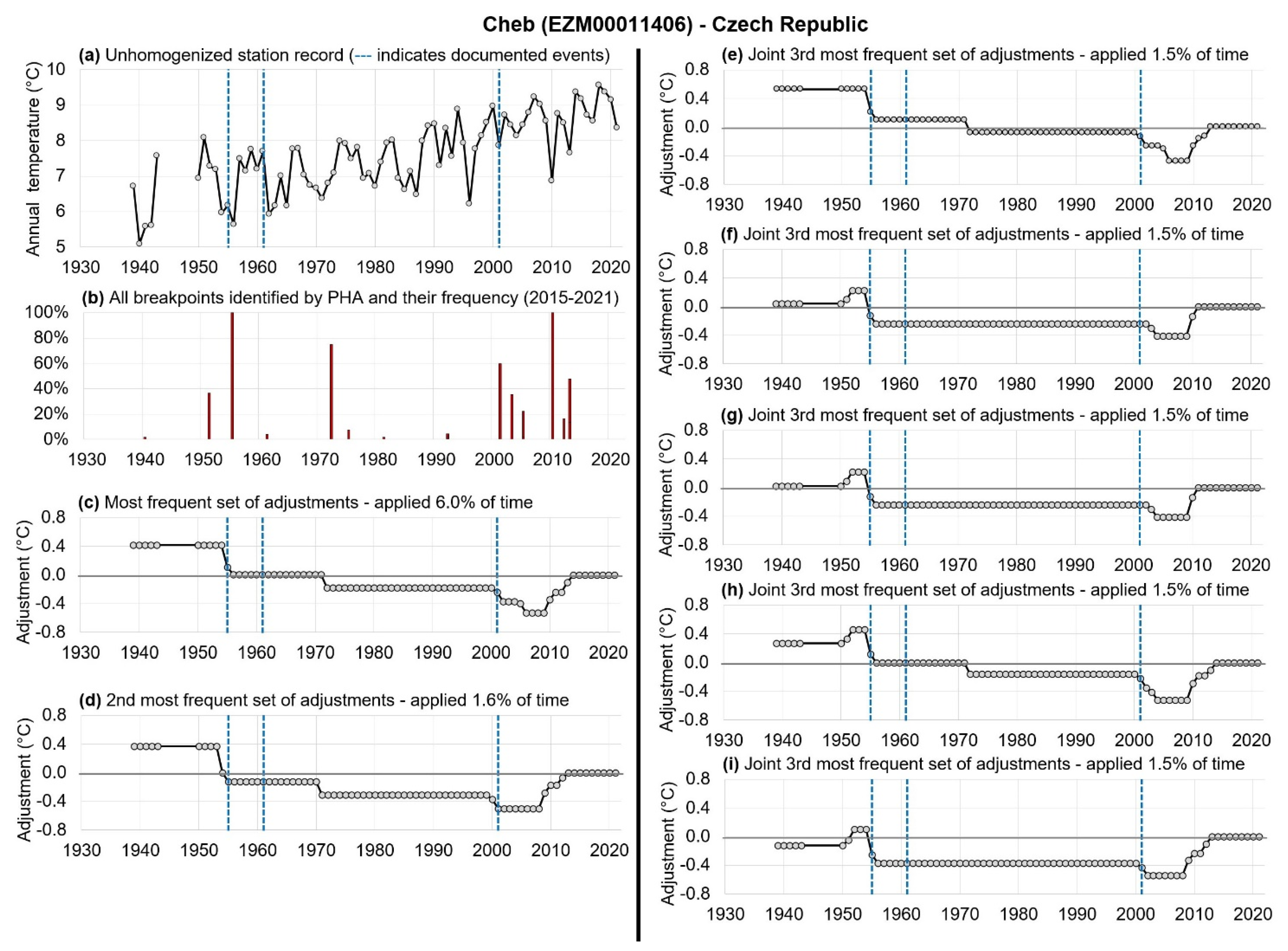
2.3. Case Study of Cheb, Czech Republic as an Example of Our Analysis Framework

As a case study, Figure 2 and Figure 3 show a detailed example of how we analyzed each station. The results are for one station record—the Version 4 record for Cheb, Czech Republic (GHCN Version 4 station ID = “EZM00011406”).

Figure 2a plots the net adjustment applied to the homogenized record (as a linear trend in °C/century) for each day’s version of the GHCN dataset. It can be seen that this metric changes quite erratically from day to day. This is a surprising result to us. We might have expected some occasional variations in the exact adjustments applied to a given station over the years, e.g., due to changes in the stations used as neighbors and monthly updates to the most recent temperature values. However, we would have still expected that the homogenization adjustments calculated by the PHA for any given station should remain fairly similar every time the algorithm is re-run.

Every time the PHA is run, the program calculates a series of breakpoints for each station record along with the magnitudes of the adjustments applied to the station record from that breakpoint to the end of the record. However, each time the PHA is re-run, the breakpoints and adjustments applied to each station record can change. On the other hand, the PHA will often recalculate the same breakpoints and adjustments that it identified on a previous run. Figure 2b plots a histogram of the “distinct sets of homogenization adjustments” that occurred for the Cheb record over the 1770 runs we analyzed. Over the 1770 runs (2015–2021), 34% of the sets of adjustments to Cheb were repeated more than 20 times, but 7% of the sets of adjustments only occurred once during the entire period.

Figure 2c presents the information conveyed in Figure 2a in histogram form, i.e., it shows the distribution of the different net homogenization adjustments applied to the Cheb record by NOAA over the 1770 runs. In this case, the average net adjustment for Cheb was relatively similar, with 59% of the net adjustments falling in the range of −0.8 °C/century to −0.5 °C/century. As will be discussed below, the breakpoints identified for this station were relatively consistent. However, even for this relatively consistent example, the net adjustments were often several tenths of a degree higher or lower.

Figure 3 provides more details on the exact adjustments applied to this station record. Three documented station history events are associated with our metadata for this station. The dates of these three events are indicated by vertical (blue) dashed lines in each of the panels except Figure 3b, and details on the events are provided in the figure caption.

Figure 3a shows the original unhomogenized station record. Figure 3b identifies any dates for which the PHA identified a breakpoint during any of the 1770 runs. In this case, the PHA collectively identified 18 different breakpoints, but not consistently so. Two of the breakpoints were identified for 100% of the runs: a cooling bias of −0.45 °C (σ = ±0.03 °C) in April 1955 (which coincided with one of the documented metadata events, i.e., a change in instrumentation) and a warming bias of +0.34 °C (σ = ±0.05 °C) in May 2010 (undocumented event). In addition, 77.2% of the runs identified a warming bias of +0.14 °C to +0.22 °C (undocumented event) on one of three similar dates (November 2012, June 2013 or August 2013). On the other hand, 7 of the 18 breakpoints were identified on less than 5% of the runs.

For this paper, we define five categories of “breakpoints” based on how frequently the PHA identifies the date as a breakpoint:

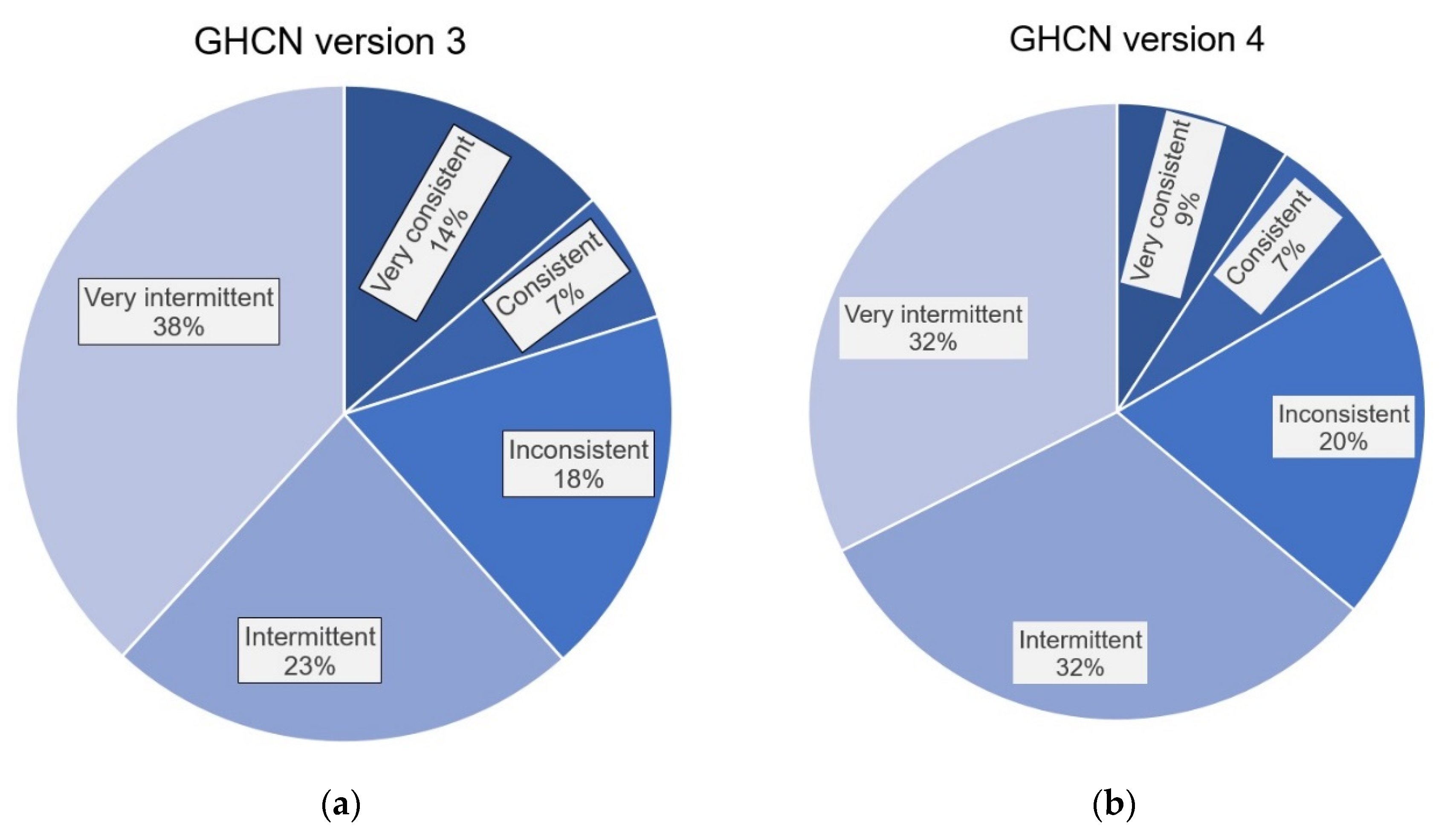
• “Very consistent”: the breakpoint was identified for >95% of the PHA runs;
• “Consistent”: the breakpoint was identified >75%, but ≤95% of the runs;
• “Inconsistent”: the breakpoint was identified for >25%, but ≤75% of the runs;
• “Intermittent”: the breakpoint was identified >5%, but ≤25% of the runs;
• “Very intermittent”: the breakpoint was identified for ≤5% of the runs;

For Cheb, the 18 breakpoints comprise: 2 “very consistent”; 5 “inconsistent”; 4 “intermittent”; and 7 “very intermittent”. Given that two of the breakpoints were “very consistent” (indeed, they occurred in 100% of the runs), the adjustments for this station are quite similar between different runs. However, as discussed above, there is quite a lot of variability in the exact set of adjustments applied in each run. In Figure 3c–i, we plot the 7 most frequently applied sets of adjustments. The adjustments of Figure 3c were applied to 107 of the 1770 runs (6.0%), Figure 3d was applied 28 times (1.6%) and the other five sets were applied 27 times each (1.5%). Therefore, they collectively describe 15.1% of the adjustments applied to the Cheb record. While the shapes of the adjustments are broadly similar, and all of the iterations include the two breakpoints mentioned above (one of which corresponds to a documented event), as mentioned before, there is still considerable variability in the overall net adjustments to the record.

The above discussion was just for one of the GHCN Version 4 stations, but should give a concrete feeling for the type of information revealed by the analysis. In the next section, we will summarize the results from all of the analyzed stations, i.e., 847 Version 4 and 249 Version 3 stations.

3. Results

Figure 4 shows the numbers of distinct sets of adjustments associated with each of the records in Version 3 (green) and Version 4 (blue). For Version 4, we can see that the majority of stations (68%) had more than 25 distinct sets of adjustments over the period of record (2015–2021, with 1812 distinct iterations of the dataset analyzed), and 14% of the stations (including Cheb described above, with 269) had more than 200 distinct sets of adjustments applied. For Version 3, the results are a bit more encouraging in that only 44% of the records had more than 25 distinct sets of adjustments and 12% had more than 200 distinct sets. Nonetheless, for both versions, there is clearly a major inconsistency in the homogenization adjustments that NOAA has applied to the GHCN station records over time.

In Figure 5, Figure 6 and Figure 7, we assess the consistency of all homogenization adjustments applied to all of the European stations we analyzed for each Version. As explained in Table 2 and Table 3, for Version 3, this comprises 1877 PHA iterations applied to 259 stations (from 24 countries). For Version 4, this comprises 1812 applied to 847 stations (again from 24 countries)

Firstly, in Figure 5, we assess the consistency of the PHA adjustments without reference to any station history metadata. Using the same categories for the consistency of breakpoints as in Section 2.3, we see that the majority of PHA adjustments were applied less than or equal to 25% of the time. For Version 3, 38% of adjustments were “very intermittent” (i.e., applied ≤5% of the time) and 23% were “intermittent” (i.e., 5–25% of the time)—Figure 5a. For Version 4, 32% were “very intermittent” and 32% were “intermittent—Figure 5b.

Only a minority of the PHA adjustments were consistently applied to the station records. For Version 3, only 14% of adjustments were “very consistent” (i.e., applied >95% of the time) and only 21% were “consistent” (i.e., 75–95% of the time)—see Figure 5a. For Version 4, only 9% were “very consistent” and only 16% were “consistent”—see Figure 5b.

As discussed in the introduction, aside from the U.S. component of the dataset (not analyzed here), the PHA is applied by NOAA to the GHCN in the absence of any station history metadata [3,4]. NOAA’s primary justification for this is that, when the station records for the GHCN were initially being compiled, the available station history metadata were very limited [2,3,4], except for the U.S. component (USHCN), which is based on data housed by NOAA [21,22,24,25]. A secondary justification is that some benchmarking simulations involving the introduction of artificial breakpoints to synthetic data have suggested that the PHA algorithm performs well at identifying many of these breakpoints without the use of “metadata” [27,34,35]. Another justification is that several studies (involving NOAA co-authors) of the USHCN dataset have argued that the PHA performs well at identifying both documented and undocumented events [21,27,29,37].

Nonetheless, in recent years, there has been a renewed interest in tracking down and digitizing station history metadata for many countries and individual stations in the recognition that this can help identify genuine non-climatic breakpoints, e.g., [46,47,48,49,50,51,52,53,54,55,56,57,58]. Unfortunately, the levels of detail and comprehensiveness of the station history metadata currently available vary substantially between countries. Some of this might be a legacy of different practices between different national meteorological services; e.g., Mamara et al. have noted that the station history metadata potentially available in the archives of the Hellenic National Meteorological Service (HNMS) are quite limited for Greece compared to some other countries [55,72]. However, they emphasize the importance of prioritizing the gathering and digitization of this information where available: “These cases demonstrate the necessity that the various meteorological services gather and digitize detailed metadata” [72].

At any rate, for this paper, we have compiled together, from multiple sources, station history metadata for 847 of the Version 4 stations and 259 of the Version 3 stations in Europe. In Figure 6, we compare how often the various breakpoints identified by NOAA for these station records coincide with any of the documented events in the corresponding metadata.

Only 3% of the PHA breakpoints for either version corresponded exactly (to the nearest month) to documented events. However, in quite a few cases only the year of an event was recorded. Furthermore, given that the PHA was being run by NOAA without any station history metadata and was relying purely on statistical techniques, it is understandable if a breakpoint is not identified accurately to the nearest month. Nonetheless, even if we consider those breakpoints identified by the PHA within 12 months of the documented event, the matches are disappointedly low: only 18% for Version 3 and 19% for Version 4.

For reference, we also show those breakpoints that loosely “match” to documented events in that the dates were within 2 years or 3 years. However, we caution that to give the “best case outcome” for the PHA, we considered a match to have occurred if any documented event coincided with the breakpoint. As a result, if two breakpoints were identified within 2 or 3 years of a given metadata event, both breakpoints might be double-counted in these categories as being “associated with” the same event even if one breakpoint occurred before the event and the other occurred after the event.

Therefore, some of the apparent “matches” within 2 or 3 years are probably spurious. Regardless, 69% of the PHA breakpoints for Version 3 stations and 67% of those for Version 4 stations had no match to any event at all within 3 years.

In Figure 7, we cross-reference the results of Figure 5 and Figure 6. That is, we compare how the consistency of a given breakpoint compares to whether it matches with documented station history events. If the consistency is better for breakpoints associated with documented events, this might offer some optimism that the PHA’s consistency could be improved using station history metadata. Disappointingly, for the Version 3 stations, there does not seem to be a clear improvement in the consistency of breakpoints based on whether they coincided with documented events. However, the results are more encouraging for Version 4, in that 39% of the very consistent breakpoints (occurring >95% of the time) had “a match” within 3 years and 28% within 1 year, whereas for the very inconsistent breakpoints (occurring ≤5% of the time) only 28% had “a match” within 3 years and only 14% had a match within 1 year. Given that the sample size was larger for Version 4 (847 stations vs. 259 in Version 3), this suggests that the consistency of the PHA adjustments to the GHCN might be partially improved if station history metadata were used.

A Case Study of the Ukrainian Results

The above discussion describes the combined results across all 24 analyzed countries. However, the exact results vary slightly from country to country. Therefore, as a case study, let us now briefly discuss the breakdown of results for one of the 24 countries —Ukraine.

In both considered versions of the GHCN dataset (Versions 3 and 4), there are multiple stations for Ukraine, one of the largest countries in Europe. Version 3 only contained 25 stations, but this has been increased to 119 for the most recent version 4. Despite the significant increase in stations in Version 4, we should note that there is still a significant portion of unused Ukrainian temperature data (especially, historical), which could increase the representativeness of the regional climate of Eastern Europe in the GHCN [56,57].

In order to evaluate the regional peculiarities of the GHCN homogenization algorithm (its detecting and adjustment parts), metadata of Ukrainian stations were collected from their historical descriptions [73,74]. For the Ukrainian metadata, this consists mainly of dates of station relocations and other non-climatic events which were clearly documented in the stations’ histories.

As discussed above, the results of the homogenization procedure for a particular station can vary significantly from day to day (i.e., from one homogenization run to another). These variations can appear as different sets of detected break points (different timing, different number), different adjustment factors, or both. It is not completely clear why this wide range of variations exists.

At any rate, for Version 3 of the dataset, the total number of break points detected in all homogenization runs is 47, while for Version 4, this quantity is considerably larger, totaling 592 (

Table 4. Break points detected in Ukrainian station series in all analyzed homogenization runs of the GHCN v3 and v4 datasets.

GHCN Version	Number of Ukrainian Station Series	Detected Break Points
		“Intermittent”, i.e., <25% of Homogenization Runs	“Inconsistent”, i.e., 25–75% of Homogenization Runs	“Consistent”, i.e., >75% of Homogenization Runs	Total
v3	25	36 (76.6% of total)	5 (10.6% of total)	6 (12.8% of total)	47 (100%)
v4	119	399 (67.4% of total)	114 (19.3% of total)	79 (13.3% of total)	592 (100%)

). This is physically explainable because in the latest version of GHCN, the higher station density has probably increased the average correlation between the time series, allowing the PHA to detect more breaks. In both versions, the majority of the detected breaks (76.6% in Version 3 and 67.4% in Version 4) can be reported as “intermittent” or “very intermittent”. They occur in less than 25% of the homogenization runs. “Inconsistent” breaks, occurring between 25 and 75% of the performed homogenizations, constitute 10.6% and 19.3% of the total detected breaks in Version 3 and 4, respectively. Only approximately 13% of the detected shifts can be considered as “consistent” or “very consistent” in both versions of the GHCN dataset, i.e., persistently occurring in more than 75% of the homogenization runs (Table 4).

An important question here is how many of the detected breaks can be confirmed by the collected metadata. In our analysis, we assumed that a break point is confirmed by some historical event when a time shift between them is not more than 1 year. The results of the comparison analysis are presented in

Table 5. Number of break points detected in Ukrainian station series of the GHCN v3 and v4 datasets, which can be confirmed by the metadata.

GHCN Version	Break Points Confirmed by Metadata
	“Intermittent”, i.e., <25% of Homogenization Runs	“Inconsistent”, i.e., 25–75% of Homogenization Runs	“Consistent”, i.e., >75% of Homogenization Runs	Total
v3	2 (5.6% of detected)	0 (0% of detected)	1 (16.7% of detected)	3 (6.4% of detected)
v4	17 (4.3% of detected)	6 (5.3% of detected)	7 (8.9% of detected)	30 (5.1% of detected)

. As can be seen from the table, only a small number of detected shifts (around 5–6% in both versions of GHCN) are associated with documented metadata events.

It is worth noting that, in other studies involving two of us (Oleg and Olesya S.), the Ukrainian monthly air temperature data (collections of 178 time series of mean, maximum and minimum temperature) has been homogenized for the period of 1946–2015 [56,57] with the HOMER software [75]. In this independent analysis, for all three datasets, the percentage of detected break points, which can be confirmed by historical events, was more than 30%. However, these results are difficult to directly compare with the PHA homogenization procedure in GHCN, because HOMER was run in a semi-automatic mode where final decisions regarding detected breaks were made by an expert.

4. Discussion

After comparing the different homogenization adjustments applied by NOAA to their widely used Global Historical Climatology Network (GHCN) monthly temperature dataset, we found a disconcerting inconsistency between the updates to the dataset from day to day. Availing of a substantial archive compiled by regularly downloading the datasets from NOAA’s website over the period 2011–2019 for version 3 and 2015-present for version 4, we assembled 1877 distinct iterations of the version 3 dataset and 1812 of the version 4 dataset which NOAA has published over the past decade.

From our large sample of station records from 24 European countries, we found that only 16% of the breakpoints and adjustments applied to the GHCN version 4 station records were repeatedly applied more than 75% of the time; 64% of the adjustments were applied to records less than 25% of the time, with 32% being applied less than 5% of the time. The results were arguably slightly better for version 3, with 21% being applied more than 75% of the time and 61% being applied less than 25% of the time. However, for version 3, 38% of the adjustments were applied less than 5% of the time.

This remarkable inconsistency in the results from NOAA’s application of the Pairwise Homogenization Algorithm (PHA) [27] to the GHCN since 2011 [3,4] is quite surprising since the PHA has performed quite well over the years against various benchmarking tests [27,34,35,36]. However, we note that those earlier assessments of the PHA were generally “one-off” assessments, i.e., they did not evaluate the consistency of the breakpoints and adjustments applied with repeated runs of the algorithm. Therefore this inconsistency of the PHA adjustments between consecutive runs would have been inadvertently overlooked by those earlier tests.

We stress that in this paper, we are definitely not criticizing the overall temperature homogenization project. We also stress that the efforts of Menne & Williams (2009) in developing the PHA [27] to try and correct for both undocumented and documented non-climatic biases were commendable. Long-term temperature records are well-known to be frequently contaminated by various non-climatic biases arising from station moves [24,61,75], changes in instrumentation [23,61], siting quality [18,19,29,31,32,33], times of observation [22,28], urbanization [18,19,25,37,38,39,42], etc. Therefore, if we are interested in using these records to study regional, hemispheric or global temperature trends, it is important to accurately account for these biases. Indeed, many of us are actively engaged in developing and/or improving the reliability of the available temperature records for Europe [18,19,35,44,45,46,49,56,57,58,59,69,70,71,75,76,77,78,79] and elsewhere [18,19,38,39] through various homogenization techniques and/or the collection of more data.

Rather, we believe these findings should be used as motivation for improving our approaches to homogenizing the available temperature records. Meanwhile, the results raise serious concerns over the reliability of the homogenized versions of the GHCN dataset, and more broadly over the PHA techniques, which do not appear to have been appreciated until now. As shown in Table 1, the homogenized GHCN datasets have been widely used by the community for studying global temperature trends. We note that PHA has also been used for homogenizing some other climatic datasets [80,81,82,83,84,85], although our analysis here is specifically on the PHA adjustments that have been applied to the GHCN datasets since 2011 [3,4].

Another major concern is how few of the adjustments are associated with documented station history metadata events—only 19% of Version 4 and 18% of Version 3 breakpoints occur within 1 year of a documented event. We agree that metadata information can sometimes be erroneous and that many events leading to non-climatic breakpoints will go undocumented [26,27,55,56,72,86,87,88,89].

So, we would expect a fraction of the breakpoints to be undocumented. However, particularly when these breakpoints are inconsistent from run to run, it raises the question, how do we know if an undocumented breakpoint that occurs for one run but not another is genuine? We are reminded of this observation by the 20th century statistician and economist, Schumacher:

“A man who uses an imaginary map, thinking that it is a true one, is likely to be worse off than someone with no map at all.”—Ernst P. Schumacher, “Small is Beautiful” (1973) [90].

With that in mind, we believe that future efforts to homogenize temperature datasets should involve a greater use of station history metadata. We appreciate that in recent years, with the commendable compilation of very large climate datasets, there has been an understandable appeal of using automated statistical homogenization techniques which do not require metadata. However, given the findings from this analysis and the above “imaginary map” problem, we suggest that, as a community, we should begin treating these “blind” homogenization results with a bit more skepticism. With that in mind, we welcome efforts to allow the use of metadata in various homogenization packages, e.g., [75,91,92], including PHA [27].

While we encourage more investigation of the various homogenization techniques via “benchmarking” experiments using synthetic data [27,34,35,36], we believe these findings highlight the importance of also benchmarking techniques against real-world data [93]. The collection and digitizing of station history metadata for as many stations as possible should be encouraged. In many cases, this could potentially be combined with the various commendable efforts to track down and digitize early instrumental thermometer records [44,46,47,48,49,53].

Finally, in this study, we have not focused on the impacts of homogenization on long-term trends. However, we note that various studies have demonstrated that the application of homogenization to a series of temperature records can inadvertently lead to the “aliasing” or “blending” of some non-climatic biases if multiple neighbors are systemically affected by similar long-term non-climatic biases, such as urbanization biases or siting biases [32,38,40]. As mentioned in the introduction, Soon et al. (2018) have suggested that one way to minimize this blending problem would be to ensure that the neighbor network used for the homogenization process is not systemically biased relative to the target stations, e.g., rural stations should be homogenized using a mostly rural station network [38].

References

1. Vose, R.S.; Schmoyer, R.L.; Steurer, P.M.; Peterson, T.C.; Heim, R.; Karl, T.R.; Eischeid, J.K. Global Historical Climatology Network, 1753–1990. ORNL DAAC 2016. [Google Scholar] [CrossRef]
2. Peterson, T.C.; Vose, R.S. An Overview of the Global Historical Climatology Network Temperature Database. Bull. Am. Meteorol. Soc. 1997, 78, 2837–2850. [Google Scholar] [CrossRef] [Green Version]
3. Lawrimore, J.H.; Menne, M.J.; Gleason, B.E.; Williams, C.N.; Wuertz, D.B.; Vose, R.S.; Rennie, J. An Overview of the Global Historical Climatology Network Monthly Mean Temperature Data Set, Version 3. J. Geophys. Res. Atmos. 2011, 116. [Google Scholar] [CrossRef]
4. Menne, M.J.; Williams, C.N.; Gleason, B.E.; Rennie, J.J.; Lawrimore, J.H. The Global Historical Climatology Network Monthly Temperature Dataset, Version 4. J. Clim. 2018, 31, 9835–9854. [Google Scholar] [CrossRef]
5. Vose, R.S.; Arndt, D.; Banzon, V.F.; Easterling, D.R.; Gleason, B.; Huang, B.; Kearns, E.; Lawrimore, J.H.; Menne, M.J.; Peterson, T.C.; et al. NOAA’s Merged Land–Ocean Surface Temperature Analysis. Bull. Am. Meteorol. Soc. 2012, 93, 1677–1685. [Google Scholar] [CrossRef]
6. Huang, B.; Menne, M.J.; Boyer, T.; Freeman, E.; Gleason, B.E.; Lawrimore, J.H.; Liu, C.; Rennie, J.J.; Schreck, C.J.; Sun, F.; et al. Uncertainty Estimates for Sea Surface Temperature and Land Surface Air Temperature in NOAAGlobalTemp Version 5. J. Clim. 2020, 33, 1351–1379. [Google Scholar] [CrossRef]
7. Hansen, J.; Ruedy, R.; Sato, M.; Lo, K. Global Surface Temperature Change. Rev. Geophys. 2010, 48. [Google Scholar] [CrossRef] [Green Version]
8. Lenssen, N.J.L.; Schmidt, G.A.; Hansen, J.E.; Menne, M.J.; Persin, A.; Ruedy, R.; Zyss, D. Improvements in the GISTEMP Uncertainty Model. J. Geophys. Res. Atmos. 2019, 124, 6307–6326. [Google Scholar] [CrossRef]
9. Japan Meteorological Agency (JMA). Tokyo Climate Center Global Average Surface Temperature Anomalies/TCC. Available online: http://ds.data.jma.go.jp/tcc/tcc/products/gwp/temp/ann_wld.html (accessed on 26 November 2021).
10. Jones, P.D.; Lister, D.H.; Osborn, T.J.; Harpham, C.; Salmon, M.; Morice, C.P. Hemispheric and Large-Scale Land-Surface Air Temperature Variations: An Extensive Revision and an Update to 2010. J. Geophys. Res. Atmos. 2012, 117. [Google Scholar] [CrossRef] [Green Version]
11. Osborn, T.J.; Jones, P.D.; Lister, D.H.; Morice, C.P.; Simpson, I.R.; Winn, J.P.; Hogan, E.; Harris, I.C. Land Surface Air Temperature Variations Across the Globe Updated to 2019: The CRUTEM5 Data Set. J. Geophys. Res. Atmos. 2021, 126, e2019JD032352. [Google Scholar] [CrossRef]
12. Sun, X.; Ren, G.; Xu, W.; Li, Q.; Ren, Y. Global Land-Surface Air Temperature Change Based on the New CMA GLSAT Data Set. Sci. Bull. 2017, 62, 236–238. [Google Scholar] [CrossRef] [Green Version]
13. Xu, W.; Li, Q.; Jones, P.; Wang, X.L.; Trewin, B.; Yang, S.; Zhu, C.; Zhai, P.; Wang, J.; Vincent, L.; et al. A New Integrated and Homogenized Global Monthly Land Surface Air Temperature Dataset for the Period since 1900. Clim. Dyn. 2018, 50, 2513–2536. [Google Scholar] [CrossRef]
14. Sun, W.; Li, Q.; Huang, B.; Cheng, J.; Song, Z.; Li, H.; Dong, W.; Zhai, P.; Jones, P. The Assessment of Global Surface Temperature Change from 1850s: The C-LSAT2.0 Ensemble and the CMST-Interim Datasets. Adv. Atmos. Sci. 2021, 38, 875–888. [Google Scholar] [CrossRef]
15. Rohde, R.; Muller, R.A.; Jacobsen, R.; Muller, E.; Perlmutter, S.; Rosenfeld, A.; Wurtele, J.; Groom, D.; Wickham, C. A New Estimate of the Average Earth Surface Land Temperature Spanning 1753 to 2011. Geoinform. Geostat. Overv. 2013, 2013. [Google Scholar] [CrossRef]
16. Rohde, R.; Muller, R.; Jacobsen, R.; Perlmutter, S.; Rosenfeld, A.; Wurtele, J.; Curry, J.; Wickham, C.; Mosher, S. Berkeley Earth Temperature Averaging Process. Geoinfor. Geostat. Overv. 2013, 2013. [Google Scholar] [CrossRef]
17. Rohde, R.A.; Hausfather, Z. The Berkeley Earth Land/Ocean Temperature Record. Earth Syst. Sci. Data 2020, 12, 3469–3479. [Google Scholar] [CrossRef]
18. Soon, W.; Connolly, R.; Connolly, M. Re-Evaluating the Role of Solar Variability on Northern Hemisphere Temperature Trends since the 19th Century. Earth-Sci. Rev. 2015, 150, 409–452. [Google Scholar] [CrossRef]
19. Connolly, R.; Soon, W.; Connolly, M.; Baliunas, S.; Berglund, J.; Butler, C.J.; Cionco, R.G.; Elias, A.G.; Fedorov, V.M.; Harde, H.; et al. How Much Has the Sun Influenced Northern Hemisphere Temperature Trends? An Ongoing Debate. Res. Astron. Astrophys. 2021, 21, 131. [Google Scholar] [CrossRef]
20. Easterling, D.R.; Karl, T.R.; Lawrimore, J.H.; Del Greco, S.A. United States Historical Climatology Network Daily Temperature and Precipitation Data (1871–1997); Oak Ridge National Lab. (ORNL): Oak Ridge, TN, USA, 2002.
21. Menne, M.J.; Williams, C.N.; Vose, R.S. The U.S. Historical Climatology Network Monthly Temperature Data, Version 2. Bull. Am. Meteorol. Soc. 2009, 90, 993–1008. [Google Scholar] [CrossRef] [Green Version]
22. Karl, T.R.; Williams, C.N.; Young, P.J.; Wendland, W.M. A Model to Estimate the Time of Observation Bias Associated with Monthly Mean Maximum, Minimum and Mean Temperatures for the United States. J. Appl. Meteorol. Climatol. 1986, 25, 145–160. [Google Scholar] [CrossRef] [Green Version]
23. Quayle, R.G.; Easterline, D.R.; Karl, T.R.; Hughes, P.Y. Effects of Recent Thermometer Changes in the Cooperative Station Network. Bull. Am. Meteorol. Soc. 1991, 72, 1718–1724. [Google Scholar] [CrossRef]
24. Karl, T.R.; Williams, C.N. An Approach to Adjusting Climatological Time Series for Discontinuous Inhomogeneities. J. Appl. Meteorol. Climatol. 1987, 26, 1744–1763. [Google Scholar] [CrossRef] [Green Version]
25. Karl, T.R.; Diaz, H.F.; Kukla, G. Urbanization: Its Detection and Effect in the United States Climate Record. J. Clim. 1988, 1, 1099–1123. [Google Scholar] [CrossRef] [Green Version]
26. Easterling, D.R.; Peterson, T.C. A New Method for Detecting Undocumented Discontinuities in Climatological Time Series. Int. J. Climatol. 1995, 15, 369–377. [Google Scholar] [CrossRef]
27. Menne, M.J.; Williams, C.N. Homogenization of Temperature Series via Pairwise Comparisons. J. Clim. 2009, 22, 1700–1717. [Google Scholar] [CrossRef] [Green Version]
28. Vose, R.S.; Williams, C.N.; Peterson, T.C.; Karl, T.R.; Easterling, D.R. An Evaluation of the Time of Observation Bias Adjustment in the U.S. Historical Climatology Network. Geophys. Res. Lett. 2003, 30. [Google Scholar] [CrossRef] [Green Version]
29. Menne, M.J.; Williams, C.N.; Palecki, M.A. On the Reliability of the U.S. Surface Temperature Record. J. Geophys. Res. Atmospheres 2010, 115. [Google Scholar] [CrossRef] [Green Version]
30. Davey, C.A.; Pielke, R.A., Sr. Microclimate Exposures of Surface-Based Weather Stations: Implications For The Assessment of Long-Term Temperature Trends. Bull. Am. Meteorol. Soc. 2005, 86, 497–504. [Google Scholar] [CrossRef] [Green Version]
31. Mahmood, R.; Foster, S.A.; Logan, D. The GeoProfile Metadata, Exposure of Instruments, and Measurement Bias in Climatic Record Revisited. Int. J. Climatol. 2006, 26, 1091–1124. [Google Scholar] [CrossRef]
32. Pielke, R.A.; Davey, C.A.; Niyogi, D.; Fall, S.; Steinweg-Woods, J.; Hubbard, K.; Lin, X.; Cai, M.; Lim, Y.-K.; Li, H.; et al. Unresolved Issues with the Assessment of Multidecadal Global Land Surface Temperature Trends. J. Geophys. Res. Atmos. 2007, 112. [Google Scholar] [CrossRef]
33. Fall, S.; Watts, A.; Nielsen-Gammon, J.; Jones, E.; Niyogi, D.; Christy, J.R.; Pielke, R.A. Analysis of the Impacts of Station Exposure on the U.S. Historical Climatology Network Temperatures and Temperature Trends. J. Geophys. Res. Atmos. 2011, 116. [Google Scholar] [CrossRef] [Green Version]
34. Williams, C.N.; Menne, M.J.; Thorne, P.W. Benchmarking the Performance of Pairwise Homogenization of Surface Temperatures in the United States. J. Geophys. Res. Atmos. 2012, 117. [Google Scholar] [CrossRef] [Green Version]
35. Venema, V.K.C.; Mestre, O.; Aguilar, E.; Auer, I.; Guijarro, J.A.; Domonkos, P.; Vertacnik, G.; Szentimrey, T.; Stepanek, P.; Zahradnicek, P.; et al. Benchmarking Homogenization Algorithms for Monthly Data. Clim. Past 2012, 8, 89–115. [Google Scholar] [CrossRef] [Green Version]
36. Domonkos, P.; Guijarro, J.A.; Venema, V.; Brunet, M.; Sigró, J. Efficiency of Time Series Homogenization: Method Comparison with 12 Monthly Temperature Test Datasets. J. Clim. 2021, 34, 2877–2891. [Google Scholar] [CrossRef]
37. Hausfather, Z.; Menne, M.J.; Williams, C.N.; Masters, T.; Broberg, R.; Jones, D. Quantifying the Effect of Urbanization on U.S. Historical Climatology Network Temperature Records. J. Geophys. Res. Atmos. 2013, 118, 481–494. [Google Scholar] [CrossRef] [Green Version]
38. Soon, W.W.-H.; Connolly, R.; Connolly, M.; O’Neill, P.; Zheng, J.; Ge, Q.; Hao, Z.; Yan, H. Comparing the Current and Early 20th Century Warm Periods in China. Earth-Sci. Rev. 2018, 185, 80–101. [Google Scholar] [CrossRef]
39. Soon, W.W.-H.; Connolly, R.; Connolly, M.; O’Neill, P.; Zheng, J.; Ge, Q.; Hao, Z.; Yan, H. Reply to Li & Yang’s Comments on “Comparing the Current and Early 20th Century Warm Periods in China”. Earth-Sci. Rev. 2019, 198, 102950. [Google Scholar] [CrossRef]
40. DeGaetano, A.T. Attributes of Several Methods for Detecting Discontinuities in Mean Temperature Series. J. Clim. 2006, 19, 838–853. [Google Scholar] [CrossRef]
41. Li, Q.; Yang, Y. Comments on “Comparing the Current and Early 20th Century Warm Periods in China” by Soon W., R. Connolly, M. Connolly et Al. Earth-Sci. Rev. 2019, 198, 102886. [Google Scholar] [CrossRef]
42. Ren, G.; Li, J.; Ren, Y.; Chu, Z.; Zhang, A.; Zhou, Y.; Zhang, L.; Zhang, Y.; Bian, T. An Integrated Procedure to Determine a Reference Station Network for Evaluating and Adjusting Urban Bias in Surface Air Temperature Data. J. Appl. Meteorol. Climatol. 2015, 54, 1248–1266. [Google Scholar] [CrossRef]
43. Ren, G.; Ding, Y.; Tang, G. An Overview of Mainland China Temperature Change Research. J. Meteorol. Res. 2017, 31, 3–16. [Google Scholar] [CrossRef]
44. Brönnimann, S.; Allan, R.; Ashcroft, L.; Baer, S.; Barriendos, M.; Brázdil, R.; Brugnara, Y.; Brunet, M.; Brunetti, M.; Chimani, B.; et al. Unlocking Pre-1850 Instrumental Meteorological Records: A Global Inventory. Bull. Am. Meteorol. Soc. 2019, 100, ES389–ES413. [Google Scholar] [CrossRef]
45. Brázdil, R.; Zahradníček, P.; Pišoft, P.; Štěpánek, P.; Bělínová, M.; Dobrovolný, P. Temperature and Precipitation Fluctuations in the Czech Republic during the Period of Instrumental Measurements. Theor. Appl. Climatol. 2012, 110, 17–34. [Google Scholar] [CrossRef]
46. Chimani, B.; Auer, I.; Prohom, M.; Nadbath, M.; Paul, A.; Rasol, D. Data Rescue in Selected Countries in Connection with the EUMETNET DARE Activity. Geosci. Data J. 2021, in press. [Google Scholar] [CrossRef]
47. Pfister, L.; Hupfer, F.; Brugnara, Y.; Munz, L.; Villiger, L.; Meyer, L.; Schwander, M.; Isotta, F.A.; Rohr, C.; Brönnimann, S. Early Instrumental Meteorological Measurements in Switzerland. Clim. Past 2019, 15, 1345–1361. [Google Scholar] [CrossRef] [Green Version]
48. Brugnara, Y.; Pfister, L.; Villiger, L.; Rohr, C.; Isotta, F.A.; Brönnimann, S. Early Instrumental Meteorological Observations in Switzerland: 1708–1873. Earth Syst. Sci. Data 2020, 12, 1179–1190. [Google Scholar] [CrossRef]
49. Skrynyk, O.; Luterbacher, J.; Allan, R.; Boichuk, D.; Sidenko, V.; Skrynyk, O.; Palarz, A.; Oshurok, D.; Xoplaki, E.; Osadchyi, V. Ukrainian Early (Pre-1850) Historical Weather Observations. Geosci. Data J. 2021, 8, 55–73. [Google Scholar] [CrossRef]
50. Mateus, C.; Potito, A.; Curley, M. Reconstruction of a Long-Term Historical Daily Maximum and Minimum Air Temperature Network Dataset for Ireland (1831–1968). Geosci. Data J. 2020, 7, 102–115. [Google Scholar] [CrossRef]
51. Kaspar, F.; Tinz, B.; Mächel, H.; Gates, L. Data Rescue of National and International Meteorological Observations at Deutscher Wetterdienst. In Proceedings of the Advances in Science and Research; 14th EMS Annual Meeting & 10th European Conference on Applied Climatology (ECAC), Prague, Czech Republic, 17 April 2015; Copernicus GmbH: Göttingen, Germany, 2015; Volume 12, pp. 57–61. [Google Scholar]
52. Camuffo, D. History of the Long Series of Daily Air Temperature in Padova (1725–1998). In Improved Understanding of Past Climatic Variability from Early Daily European Instrumental Sources; Camuffo, D., Jones, P., Eds.; Springer: Dordrecht, The Netherlands, 2002; pp. 7–75. ISBN 978-94-010-0371-1. [Google Scholar]
53. Camuffo, D.; Bertolin, C. Recovery of the Early Period of Long Instrumental Time Series of Air Temperature in Padua, Italy (1716–2007). Phys. Chem. Earth Parts ABC 2012, 40–41, 23–31. [Google Scholar] [CrossRef]
54. Kuglitsch, F.G.; Auchmann, R.; Bleisch, R.; Brönnimann, S.; Martius, O.; Stewart, M. Break Detection of Annual Swiss Temperature Series. J. Geophys. Res. Atmos. 2012, 117. [Google Scholar] [CrossRef] [Green Version]
55. Mamara, A.; Argiriou, A.A.; Anadranistakis, M. Detection and Correction of Inhomogeneities in Greek Climate Temperature Series. Int. J. Climatol. 2014, 34, 3024–3043. [Google Scholar] [CrossRef]
56. Osadchyi, V.; Skrynyk, O.; Radchenko, R.; Skrynyk, O. Homogenization of Ukrainian Air Temperature Data. Int. J. Climatol. 2018, 38, 497–505. [Google Scholar] [CrossRef]
57. Skrynyk, O.; Aguilar, E.; Skrynyk, O.; Sidenko, V.; Boichuk, D.; Osadchyi, V. Quality Control and Homogenization of Monthly Extreme Air Temperature of Ukraine. Int. J. Climatol. 2019, 39, 2071–2079. [Google Scholar] [CrossRef]
58. Pospieszyńska, A.; Przybylak, R. Air Temperature Changes in Toruń (Central Poland) from 1871 to 2010. Theor. Appl. Climatol. 2019, 135, 707–724. [Google Scholar] [CrossRef] [Green Version]
59. Przybylak, R. The Climate of Poland in Recent Centuries: A Synthesis of Current Knowledge: Instrumental Observations. In The Polish Climate in the European Context: An Historical Overview; Przybylak, R., Majorowicz, J., Brázdil, R., Kejna, M., Eds.; Springer: Berlin/Heidelberg, Germany, 2010; pp. 129–166. ISBN 978-90-481-3167-9. [Google Scholar]
60. Butler, C.J.; García Suárez, A.M.; Coughlin, A.D.S.; Morrell, C. Air Temperatures at Armagh Observatory, Northern Ireland, from 1796 to 2002. Int. J. Climatol. 2005, 25, 1055–1079. [Google Scholar] [CrossRef] [Green Version]
61. Keevallik, S.; Vint, K. Influence of Changes in the Station Location and Measurement Routine on the Homogeneity of the Temperature, Wind Speed and Precipitation Time Series. Est. J. Eng. 2012, 18, 302–313. [Google Scholar] [CrossRef] [Green Version]
62. Moberg, A.; Bergström, H. Homogenization of Swedish Temperature Data. Part III: The Long Temperature Records from Uppsala and Stockholm. Int. J. Climatol. 1997, 17, 667–699. [Google Scholar] [CrossRef]
63. Moberg, A.; Alexandersson, H.; Bergström, H.; Jones, P.D. Were Southern Swedish Summer Temperatures before 1860 as Warm as Measured? Int. J. Climatol. 2003, 23, 1495–1521. [Google Scholar] [CrossRef]
64. Bryś, K.; Bryś, T. Reconstruction of the 217-Year (1791–2007) Wrocław Air Temperature and Precipitation Series. Bull. Geogr. Phys. Geogr. Ser. 2010, 3, 121–171. [Google Scholar] [CrossRef] [Green Version]
65. Burt, S.; Burt, T. Oxford Weather and Climate Since 1767; Oxford University Press: Oxford, UK, 2019; ISBN 978-0-19-883463-2. [Google Scholar]
66. Cappelen, J.; Kern-Hansen, C.; Laursen, E.V.; Jørgensen, P.V.; Jørgensen, B.V. Denmark—DMI Historical Climate Data Collection 1768–2019; Danish Meteorological Institute: Copenhagen, Denmark, 2020; p. 112. Available online: https://www.dmi.dk/fileadmin/user_upload/Rapporter/TR/2020/DMIRep20-02.pdf (accessed on 12 January 2022).
67. Lundstad, E.; Tveito, O.E. Homogenization of Daily Mean Temperature in Norway; DNMI, Norwegian Meteorological Institute: Oslo, Norway, 2016; p. 78. Available online: https://www.met.no/publikasjoner/met-report/met-report-2016/ (accessed on 12 January 2022).
68. Khasandi Kuya, E.; Gjelten, H.M.; Tveito, O.E. Homogenization of Norway’s Mean Monthly Temperature Series; MET Report No. 3/2020; Norwegian Meteorological Institute: Oslo, Norway, 2020; p. 95. Available online: https://www.met.no/sokeresultat/ (accessed on 12 January 2022).
69. Nojarov, P. Changes in Air Temperatures and Atmosphere Circulation in High Mountainous Parts of Bulgaria for the Period 1941–2008. J. Mt. Sci. 2012, 9, 185–200. [Google Scholar] [CrossRef]
70. Nojarov, P. Atmospheric Circulation as a Factor for Air Temperatures in Bulgaria. Meteorol. Atmos. Phys. 2014, 125, 145–158. [Google Scholar] [CrossRef]
71. Nojarov, P. Factors Affecting Air Temperature in Bulgaria. Theor. Appl. Climatol. 2019, 137, 571–586. [Google Scholar] [CrossRef]
72. Mamara, A.; Argiriou, A.A.; Anadranistakis, M. Homogenization of Mean Monthly Temperature Time Series of Greece. Int. J. Climatol. 2013, 33, 2649–2666. [Google Scholar] [CrossRef]
73. KHMO (Kiev Hydrometeorological Observatory). History and Physico-Geographical Description of Meteorological Stations; Climatological Handbook USSR, Issue 10, Ukrainian SSR; KHMO: Kiev, Ukraine, 1968. (In Russian) [Google Scholar]
74. CGO (Central Geophysical Observatory, formerly KHMO). History and Physiographic Description of Ukrainian Meteorological Stations; Climatological Handbook; CGO: Kyiv, Ukraine, 2011. (In Ukrainian) [Google Scholar]
75. Mestre, O.; Domonkos, P.; Picard, F.; Auer, I.; Robin, S.; Lebarbier, E.; Boehm, R.; Aguilar, E.; Guijarro, J.; Vertachnik, G.; et al. HOMER: A Homogenization Software—Methods and Applications. Idojaras 2013, 117, 47–67. [Google Scholar]
76. Dijkstra, F.; de Vos, R.; Ruis, J.; Crok, M. Reassessment of the Homogenization of Daily Maximum Temperatures in the Netherlands since 1901. Theor. Appl. Climatol. 2021. [Google Scholar] [CrossRef]
77. Spinoni, J.; Szalai, S.; Szentimrey, T.; Lakatos, M.; Bihari, Z.; Nagy, A.; Németh, Á.; Kovács, T.; Mihic, D.; Dacic, M.; et al. Climate of the Carpathian Region in the Period 1961–2010: Climatologies and Trends of 10 Variables. Int. J. Climatol. 2015, 35, 1322–1341. [Google Scholar] [CrossRef] [Green Version]
78. Brugnara, Y.; Auchmann, R.; Brönnimann, S.; Allan, R.J.; Auer, I.; Barriendos, M.; Bergström, H.; Bhend, J.; Brázdil, R.; Compo, G.P.; et al. A Collection of Sub-Daily Pressure and Temperature Observations for the Early Instrumental Period with a Focus on the “Year without a Summer” 1816. Clim. Past 2015, 11, 1027–1047. [Google Scholar] [CrossRef] [Green Version]
79. Wypych, A.; Ustrnul, Z.; Schmatz, D.R. Long-Term Variability of Air Temperature and Precipitation Conditions in the Polish Carpathians. J. Mt. Sci. 2018, 15, 237–253. [Google Scholar] [CrossRef]
80. Dunn, R.J.H.; Willett, K.M.; Morice, C.P.; Parker, D.E. Pairwise Homogeneity Assessment of HadISD. Clim. Past 2014, 10, 1501–1522. [Google Scholar] [CrossRef] [Green Version]
81. Dunn, R.J.H.; Willett, K.M.; Parker, D.E.; Mitchell, L. Expanding HadISD: Quality-Controlled, Sub-Daily Station Data from 1931. Geosci. Instrum. Methods Data Syst. 2016, 5, 473–491. [Google Scholar] [CrossRef] [Green Version]
82. Willett, K.M.; Dunn, R.J.H.; Thorne, P.W.; Bell, S.; de Podesta, M.; Parker, D.E.; Jones, P.D.; Williams, C.N., Jr. HadISDH Land Surface Multi-Variable Humidity and Temperature Record for Climate Monitoring. Clim. Past 2014, 10, 1983–2006. [Google Scholar] [CrossRef] [Green Version]
83. Thorne, P.W.; Menne, M.J.; Williams, C.N.; Rennie, J.J.; Lawrimore, J.H.; Vose, R.S.; Peterson, T.C.; Durre, I.; Davy, R.; Esau, I.; et al. Reassessing Changes in Diurnal Temperature Range: A New Data Set and Characterization of Data Biases. J. Geophys. Res. Atmos. 2016, 121, 5115–5137. [Google Scholar] [CrossRef]
84. Trewin, B. A Daily Homogenized Temperature Data Set for Australia. Int. J. Climatol. 2013, 33, 1510–1529. [Google Scholar] [CrossRef]
85. Trewin, B.; Braganza, K.; Fawcett, R.; Grainger, S.; Jovanovic, B.; Jones, D.; Martin, D.; Smalley, R.; Webb, V. An Updated Long-Term Homogenized Daily Temperature Data Set for Australia. Geosci. Data J. 2020, 7, 149–169. [Google Scholar] [CrossRef]
86. Venema, V.; Trewin, B.; Wang, X.; Szentimrey, T.; Lakatos, M.; Aguilar, E.; Auer, I.; Guijarro, J.A.; Menne, M.; Oria, C. Guidance on the Homogenization of Climate Station Data. 2018. Available online: https://eartharxiv.org/repository/view/1158/ (accessed on 12 January 2022).
87. Mitchell, J.M., Jr. On the Causes of Instrumentally Observed Secular Temperature Trends. J. Atmos. Sci. 1953, 10, 244–261. [Google Scholar] [CrossRef] [Green Version]
88. Vertačnik, G.; Dolinar, M.; Bertalanič, R.; Klančar, M.; Dvoršek, D.; Nadbath, M. Ensemble Homogenization of Slovenian Monthly Air Temperature Series. Int. J. Climatol. 2015, 35, 4015–4026. [Google Scholar] [CrossRef]
89. Yosef, Y.; Aguilar, E.; Alpert, P. Detecting and Adjusting Artificial Biases of Long-Term Temperature Records in Israel. Int. J. Climatol. 2018, 38, 3273–3289. [Google Scholar] [CrossRef]
90. Schumacher, E.F. Small Is Beautiful: Economics as If People Mattered; Reprint ed.; (Original 1973); Harper Perennial: New York, NY, USA, 2010; ISBN 978-0-06-199776-1. [Google Scholar]
91. Domonkos, P. Combination of Using Pairwise Comparisons and Composite Reference Series: A New Approach in the Homogenization of Climatic Time Series with ACMANT. Atmosphere 2021, 12, 1134. [Google Scholar] [CrossRef]
92. Wang, X.; Feng, Y. RHtestsV4 User Manual. Environment Canada Science and Technology Branch Atmospheric Science and Technology Directorate Climate Research. Div. Res. Rep. 2013. Available online: http://etccdi.pacificclimate.org/RHtest/RHtestsV4_UserManual_10Dec2014.pdf (accessed on 12 January 2022).
93. Squintu, A.A.; van der Schrier, G.; Štěpánek, P.; Zahradníček, P.; Tank, A.K. Comparison of Homogenization Methods for Daily Temperature Series against an Observation-Based Benchmark Dataset. Theor. Appl. Climatol. 2020, 140, 285–301. [Google Scholar] [CrossRef] [Green Version]
Figure 1. Locations of all the European Global Historical Climatology Network (GHCN) stations. Filled red circles correspond to the stations analyzed in this paper. These are the stations for which we obtained station history metadata. Hollow grey circles correspond to any other stations in the dataset. (a) Version 3 of the GHCN dataset; (b) Version 4 of the GHCN dataset.
Atmosphere 13 00285 g001
Figure 2. Breakdown of the 1770 homogenizations applied by NOAA to the Cheb (EZM00011406), Czech Republic, Version 4 station over the period of analysis for this study, i.e., 2015–2021. Out of these 1770 homogenizations, 269 distinct sets of adjustments were applied on various different dates; (a) shows the net effect (in °C/century) of the homogenization adjustments applied to the station record on each day’s run of the homogenization algorithm; (b) shows how often each of the distinct sets of homogenization adjustments were applied to the station record by NOAA; (c) shows the distribution of homogenization adjustments applied—binned according to the net adjustment to the record.
Atmosphere 13 00285 g002
Figure 3. The Cheb (EZM00011406), Czech Republic, station as a case study of the types of homogenization adjustments applied to the Global Historical Climatology Network (GHCN) stations. These are the results for the Version 4 station which was homogenized 1770 times by NOAA over the period of analysis for this study, i.e., 2015–2021. Out of these 1770 homogenizations, 269 distinct sets of adjustments were applied on different dates. Three documented events are associated with this station according to the historical metadata: (i) a change in instrumentation in January 1955; (ii) a station move in January 1961 and (iii) a station move and change in instrumentation from manual to automated weather station in January 2001. These dates are indicated with vertical dashed (blue) lines. (a) shows the unhomogenized station record; (b) shows all of the breakpoints identified by NOAA during any homogenization, along with how often the breakpoints were identified; (c) shows the most frequent of the 269 distinct sets of adjustments applied by NOAA—applied in 6.0% of the iterations;); (d) shows the next most frequent—applied to 1.6% of the iterations; (ei) show the six next most frequent—each applied to 1.5% of the iterations.
Atmosphere 13 00285 g003
Figure 4. Summary of the numbers of distinct homogenization adjustments applied to the analyzed European stations for Version 3 (green) and Version 4 (blue) of the homogenized GHCN datasets over the period of analysis. For Version 3, Table 1877. distinct datasets analyzed (2011–2019) while for Version 4, there were 1812 (2015–2021). (a) Binned histogram showing the percentage of stations in each bin (of size 25); (b) cumulative histogram of the same data.
Atmosphere 13 00285 g004
Figure 5. Breakdown of how consistent the PHA adjustments applied to the European Global Historical Climatology Network (GHCN) stations are when considered over all iterations analyzed. “Very consistent” adjustments were repeatedly identified by the PHA for >95% of the iterations; “Consistent” was ≤95%, but >75%; “Inconsistent” was ≤75%, but >25%; “Intermittent” was ≤25%, but >5%; “Very intermittent” was ≤5%. (a) Version 3 of the GHCN dataset; (b) Version 4 of the GHCN dataset.
Atmosphere 13 00285 g005
Figure 6. Breakdown of how often the PHA adjustments for a station corresponded to a documented event in the station history metadata. “Exact match” refers to breakpoints that occurred for the same month as a documented event, whereas “No match” indicates that there was no documented event within 3 years of the breakpoint. Note that if the date of a documented event was only known to the nearest year, the date was approximated to June of that year, i.e., month 6. (a) Version 3 of the GHCN dataset; (b) Version 4 of the GHCN dataset.
Atmosphere 13 00285 g006
Figure 7. Relationship between the consistency of the PHA adjustments and how closely the breakpoints corresponded to a documented event in the station history metadata. (a) Version 3 of the GHCN dataset; (b) Version 4 of the GHCN dataset.
Atmosphere 13 00285 g007