
High Spatial Resolution Assessment of the Effect of the Spanish National Air Pollution Control Programme on Street-Level NO2 Concentrations in Three Neighborhoods of Madrid (Spain) Using Mesoscale and CFD Modelling

 , ,
, ,  , , ,
, , ,  ,
,  and
and 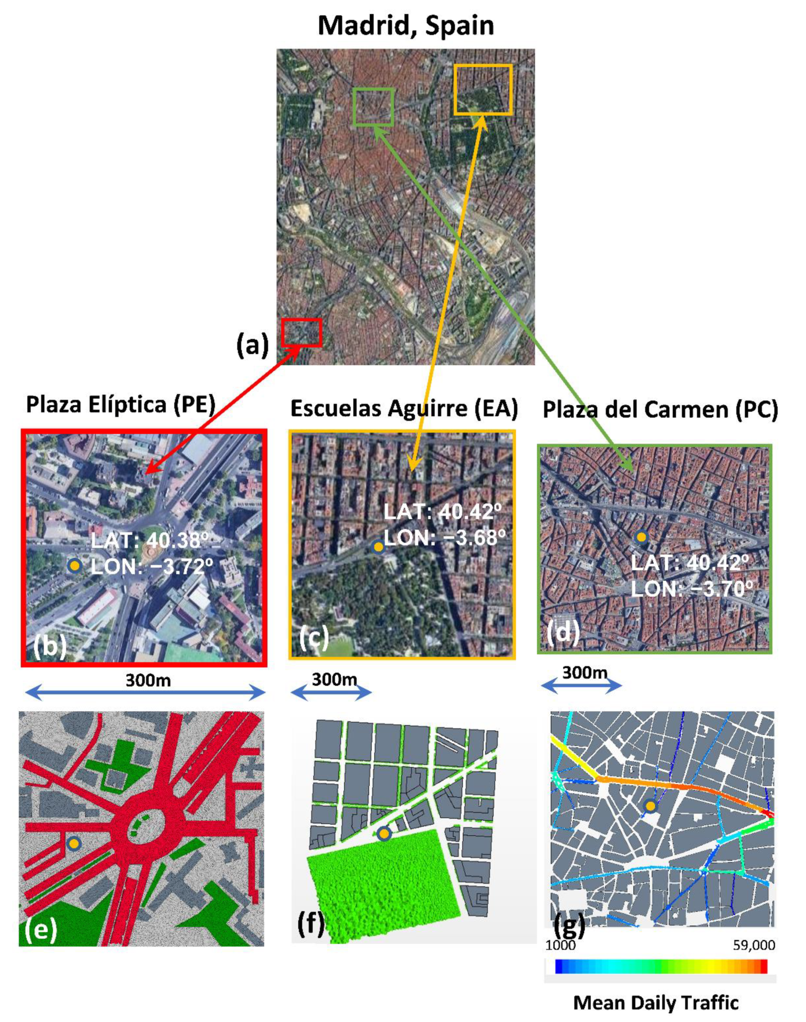
Abstract
:1. Introduction
2. Materials and Methods
2.1. Description of the Study Urban Areas
2.2. NO2 Concentration Modelling
2.2.1. CFD Model Description and Set-Up
2.2.2. Methodology for Estimating Annual Average Concentration
3. Results
3.1. Evaluation of the Modelling Appproach
3.2. Impacts of Emission Reduction Scenarios on NO2 Concentrations
4. Discussion and Conclusions
Author Contributions
Funding
Institutional Review Board Statement
Informed Consent Statement
Data Availability Statement
Acknowledgments
Conflicts of Interest
References
- European Environment Agency. Air Quality in Europe 2021 Report; EEA Report No 15/2021; European Environment Agency, Publications Office of the European Union: Luxembourg, 2021.
- Vivanco, M.G.; Garrido, J.L.; Martín, F.; Theobald, M.R.; Gil, V.; Santiago, J.-L.; Lechón, Y.; Gamarra, A.R.; Sánchez, E.; Alberto, A.; et al. Assessment of the effects of the spanish national air pollution control programme on air quality. Atmosphere 2021, 12, 158. [Google Scholar] [CrossRef]
- Santiago, J.L.; Borge, R.; Sanchez, B.; Quaassdorff, C.; de la Paz, D.; Martilli, A.; Rivas, E.; Martín, F. Estimates of pedestrian exposure to atmospheric pollution using high-resolution modelling in a real traffic hot-spot. Sci. Total Environ. 2021, 755, 142475. [Google Scholar] [CrossRef] [PubMed]
- Santiago, J.L.; Rivas, E.; Gamarra, A.R.; Vivanco, M.G.; Buccolieri, R.; Martilli, A.; Lechón, Y.; Martín, F. Estimates of population exposure to atmospheric pollution and health-related externalities in a real city: The impact of spatial resolution on the accuracy of results. Sci. Total Environ. 2021; 152062, in press, published on-line. [Google Scholar] [CrossRef] [PubMed]
- Borge, R.; Narros, A.; Artíñano, B.; Yagüe, C.; Gómez-Moreno, F.J.; de la Paz, D.; Román-Cascón, C.; Díaz, E.; Maqueda, G.; Sastre, M.; et al. Assessment of microscale spatio-temporal variation of air pollution at an urban hotspot in Madrid (Spain) through an extensive field campaign. Atmos. Environ. 2016, 140, 432–445. [Google Scholar] [CrossRef]
- Beauchamp, M.; Malherbe, L.; de Fouquet, C.; Létinois, L. A necessary distinction between spatial representativeness of an air quality monitoring station and the delimitation of exceedance areas. Environ. Monit. Assess. 2018, 190, 1–27. [Google Scholar] [CrossRef]
- Vardoulakis, S.; Solazzo, E.; Lumbreras, J. Intra-urban and street scale variability of BTEX, NO2 and O3 in Birmingham, UK: Implications for exposure assessment. Atmos. Environ. 2011, 45, 5069–5078. [Google Scholar] [CrossRef]
- Vardoulakis, S.; Fisher, B.E.; Pericleous, K.; Gonzalez-Flesca, N. Modelling air quality in street canyons: A review. Atmos. Environ. 2003, 37, 155–182. [Google Scholar] [CrossRef] [Green Version]
- Vardoulakis, S.; Dimitrova, R.; Richards, K.; Hamlyn, D.; Camilleri, G.; Weeks, M.; Sini, J.-F.; Britter, R.; Borrego, C.; Schatzmann, M.; et al. Numerical model inter-comparison for wind flow and turbulence around single-block buildings. Environ. Model. Assess. 2011, 16, 169–181. [Google Scholar] [CrossRef]
- Buccolieri, R.; Salim, S.M.; Leo, L.S.; Di Sabatino, S.; Chan, A.; Ielpo, P.; Gromke, C. Analysis of local scale tree–atmosphere interaction on pollutant concentration in idealized street canyons and application to a real urban junction. Atmos. Environ. 2011, 45, 1702–1713. [Google Scholar] [CrossRef]
- Amorim, J.H.; Rodrigues, V.; Tavares, R.; Valente, J.; Borrego, C. CFD modelling of the aerodynamic effect of trees on urban air pollution dispersion. Sci. Total Environ. 2013, 461, 541–551. [Google Scholar] [CrossRef]
- Vos, P.E.; Maiheu, B.; Vankerkom, J.; Janssen, S. Improving local air quality in cities: To tree or not to tree? Environ. Pollut. 2013, 183, 113–122. [Google Scholar] [CrossRef] [PubMed]
- Gromke, C.; Blocken, B. Influence of avenue-trees on air quality at the urban neighborhood scale. Part II: Traffic pollutant concentrations at pedestrian level. Environ. Pollut. 2015, 196, 176–184. [Google Scholar] [CrossRef] [PubMed] [Green Version]
- Jeanjean, A.P.; Buccolieri, R.; Eddy, J.; Monks, P.S.; Leigh, R.J. Air quality affected by trees in real street canyons: The case of Marylebone neighbourhood in central London. Urban For. Urban Green. 2017, 22, 41–53. [Google Scholar] [CrossRef]
- Santiago, J.L.; Borge, R.; Martin, F.; de la Paz, D.; Martilli, A.; Lumbreras, J.; Sanchez, B. Evaluation of a CFD-based approach to estimate pollutant distribution within a real urban canopy by means of passive samplers. Sci. Total Environ. 2017, 576, 46–58. [Google Scholar] [CrossRef]
- Santiago, J.L.; Sanchez, B.; Quaassdorff, C.; de la Paz, D.; Martilli, A.; Martín, F.; Borge, R.; Rivas, E.; Gómez-Moreno, F.J.; Días, E.; et al. Performance evaluation of a multiscale modelling system applied to particulate matter dispersion in a real traffic hot spot in Madrid (Spain). Atmos. Pollut. Res. 2020, 11, 141–155. [Google Scholar] [CrossRef]
- Rivas, E.; Santiago, J.L.; Lechón, Y.; Martín, F.; Ariño, A.; Pons, J.J.; Santamaría, J.M. CFD modelling of air quality in Pamplona City (Spain): Assessment, stations spatial representativeness and health impacts valuation. Sci. Total Environ. 2019, 649, 1362–1380. [Google Scholar] [CrossRef]
- Santiago, J.L.; Martín, F.; Martilli, A. A computational fluid dynamic modelling approach to assess the representativeness of urban monitoring stations. Sci. Total Environ. 2013, 454–455, 61–72. [Google Scholar] [CrossRef]
- Martín, F.; Santiago, J.L.; Kracht, O.; García, L.; Gerboles, M. FAIRMODE Spatial Representativeness Feasibility Study; Publications Office of the European Union: Luxembourg, 2021. [Google Scholar]
- Santiago, J.L.; Martin, F. Use of CFD modeling for estimating spatial representativeness of urban air pollution monitoring sites and suitability of their locations. Física de a Tierra 2015, 27, 191. [Google Scholar]
- Kwak, K.H.; Baik, J.J.; Ryu, Y.H.; Lee, S.H. Urban air quality simulation in a high-rise building area using a CFD model coupled with mesoscale meteorological and chemistry-transport models. Atmos. Environ. 2015, 100, 167–177. [Google Scholar] [CrossRef]
- Sanchez, B.; Santiago, J.L.; Martilli, A.; Martin, F.; Borge, R.; Quaassdorff, C.; de la Paz, D. Modelling NOx concentrations through CFD-RANS in an urban hot-spot using high resolution traffic emissions and meteorology from a mesoscale model. Atmos. Environ. 2017, 163, 155–165. [Google Scholar] [CrossRef]
- Santiago, J.L.; Rivas, E.; Sanchez, B.; Buccolieri, R.; Martin, F. The impact of planting trees on NOx concentrations: The case of the Plaza de la Cruz neighborhood in Pamplona (Spain). Atmosphere 2017, 8, 131. [Google Scholar] [CrossRef] [Green Version]
- Buccolieri, R.; Santiago, J.L.; Rivas, E.; Sanchez, B. Review on urban tree modelling in CFD simulations: Aerodynamic, deposition and thermal effects. Urban For. Urban Green. 2018, 31, 212–220. [Google Scholar] [CrossRef]
- Borge, R.; Artíñano, B.; Yagüe, C.; Gomez-Moreno, F.J.; Saiz-Lopez, A.; Sastre, M.; Narros, A.; García-Nieto, D.; Benavent, N.; Maqueda, G.; et al. Application of a short term air quality action plan in Madrid (Spain) under a high-pollution episode-Part I: Diagnostic and analysis from observations. Sci. Total Environ. 2018, 635, 1561–1573. [Google Scholar] [CrossRef] [PubMed]
- Parra, M.A.; Santiago, J.L.; Martín, F.; Martilli, A.; Santamaría, J.M. A methodology to urban air quality assessment during large time periods of winter using computational fluid dynamic models. Atmos. Environ. 2010, 44, 2089–2097. [Google Scholar] [CrossRef]
- Solazzo, E.; Vardoulakis, S.; Cai, X. A novel methodology for interpreting air quality measurements from urban streets using CFD modelling. Atmos. Environ. 2011, 45, 5230–5239. [Google Scholar] [CrossRef]
- Vranckx, S.; Vos, P.; Maiheu, B.; Janssen, S. Impact of trees on pollutant dispersion in street canyons: A numerical study of the annual average effects in Antwerp, Belgium. Sci. Total Environ. 2015, 532, 474–483. [Google Scholar] [CrossRef]
- Reiminger, N.; Jurado, X.; Vazquez, J.; Wemmert, C.; Blond, N.; Wertel, J.; Dufresne, M. Methodologies to assess mean annual air pollution concentration combining numerical results and wind roses. Sustain. Cities Soc. 2020, 59, 102221. [Google Scholar] [CrossRef]
- Rafael, S.; Rodrigues, V.; Oliveira, K.; Coelho, S.; Lopes, M. How to compute long-term averages for air quality assessment at urban areas? Sci. Total Environ. 2021, 795, 148603. [Google Scholar] [CrossRef]
- Gamarra, A.R.; Lechón, Y.; Vivanco, M.G.; Garrido, J.L.; Martín, F.; Sánchez, E.; Theobald, M.R.; Gil, V.; Santiago, J.L. Benefit Analysis of the 1st Spanish Air Pollution Control Programme on Health Impacts and Associated Externalities. Atmosphere 2021, 12, 32. [Google Scholar] [CrossRef]
- Madrid City Council. Madrid 2016 Annual Air Quality Assessment Report (Calidad del aire Madrid 2016); General Directorate of Sustainability and Environmental Control, Madrid City Council, 2016; Available online: http://www.mambiente.munimadrid.es/opencms/export/sites/default/calaire/Anexos/Memorias/Memoria2016.pdf (accessed on 10 January 2022).
- Santiago, J.-L.; Martilli, A.; Martin, F. On Dry Deposition Modelling of Atmospheric Pollutants on Vegetation at the Microscale: Application to the Impact of Street Vegetation on Air Quality. Bound.-Layer Meteorol. 2017, 162, 451–474. [Google Scholar] [CrossRef]
- Santiago, J.-L.; Buccolieri, R.; Rivas, E.; Calvete-Sogo, H.; Sanchez, B.; Martilli, A.; Alonso, R.; Elustondo, D.; Santamaría, J.M.; Martin, F. CFD modelling of vegetation barrier effects on the reduction of traffic-related pollutant concentration in an avenue of Pamplona, Spain. Sustain. Cities Soc. 2019, 48, 101559. [Google Scholar] [CrossRef]
- Tominaga, Y.; Stathopoulos, T. Turbulent Schmidt numbers for CFD analysis with various types of flowfield. Atmos. Environ. 2007, 41, 8091–8099. [Google Scholar] [CrossRef]
- Franke, J.; Schlünzen, H.; Carissimo, B. Best Practice Guideline for the CFD Simulation of Flows in the Urban Environment. In COST Action 732—Quality Assurance and Improvement of Microscale Meteorological Models; Meteorological Institute, University of Hamburg (Germany): Hamburg, Germany, 2007; ISBN 3-00-018312-4. [Google Scholar]
- Richards, P.J.; Hoxey, R.P. Appropriate boundary conditions for computational wind engineering models using the k-ϵ turbulence model. J. Wind Eng. Ind. Aerodyn. 1993, 46, 145–153. [Google Scholar] [CrossRef]
- Sanchez, B.; Quaassdorff, C.; Santiago, J.L.; Borge, R.; Martin, F.; de la Paz, D.; Martilli, A.; Rivas, E. Effects of traffic emission resolution on NOx concentration obtained by CFD-RANS modelling over a real urban area in Madrid (Spain). In Proceedings of the HARMO17 Conference, Budapest, Hungary, 9–12 May 2016. [Google Scholar]
- Sanchez, B.; Santiago, J.L.; Martilli, A.; Palacios, M.; Kirchner, F. CFD modeling of reactive pollutant dispersion in simplified urban configurations with different chemical mechanisms. Atmos. Chem. Phys. 2016, 16, 12143–12157. [Google Scholar] [CrossRef] [Green Version]
- Menut, L.; Bessagnet, B.; Khvorostyanov, D.; Beekmann, M.; Blond, N.; Colette, A.; Coll, I.; Curci, G.; Foret, G.; Hodzic, A.; et al. CHIMERE 2013: A model for regional atmospheric composition modelling. Geosci. Model Dev. 2013, 6, 981–1028. [Google Scholar] [CrossRef] [Green Version]
- Gromke, C.; Buccolieri, R.; Di Sabatino, S.; Ruck, B. Dispersion study in a street canyon with tree planting by means of wind tunnel and numerical investigations—Evaluation of CFD data with experimental data. Atmos. Environ. 2008, 42, 8640–8650. [Google Scholar] [CrossRef]
- Quaassdorff, C.; Borge, R.; Pérez, J.; Lumbreras, J.; de la Paz, D.; de Andrés, J.M. Microscale traffic simulation and emission estimation in a heavily trafficked roundabout in Madrid (Spain). Sci. Total Environ. 2016, 566, 416–427. [Google Scholar] [CrossRef]
- Holman, C.; Harrison, R.; Querol, X. Review of the efficacy of low emission zones to improve urban air quality in European cities. Atmos. Environ. 2015, 111, 161–169. [Google Scholar] [CrossRef]
- Abhijith, K.V.; Kumar, P.; Gallagher, J.; McNabola, A.; Baldauf, R.; Pilla, F.; Broderick, B.; Di Sabatino, S.; Pulvirenti, B. Air pollution abatement performances of green infrastructure in open road and built-up street canyon environments-A review. Atmos. Environ. 2017, 162, 71–86. [Google Scholar] [CrossRef]
- Buccolieri, R.; Savio Carlo, O.; Rivas, E.; Santiago, J.L. Urban Obstacles Influence on Street Canyon Ventilation: A Brief Review. Environ. Sci. Proc. 2021, 8, 11. [Google Scholar] [CrossRef]


Publisher’s Note: MDPI stays neutral with regard to jurisdictional claims in published maps and institutional affiliations. |
© 2022 by the authors. Licensee MDPI, Basel, Switzerland. This article is an open access article distributed under the terms and conditions of the Creative Commons Attribution (CC BY) license (https://creativecommons.org/licenses/by/4.0/).
Share and Cite
Santiago, J.-L.; Sanchez, B.; Rivas, E.; Vivanco, M.G.; Theobald, M.R.; Garrido, J.L.; Gil, V.; Martilli, A.; Rodríguez-Sánchez, A.; Buccolieri, R.; et al. High Spatial Resolution Assessment of the Effect of the Spanish National Air Pollution Control Programme on Street-Level NO2 Concentrations in Three Neighborhoods of Madrid (Spain) Using Mesoscale and CFD Modelling. Atmosphere 2022, 13, 248. https://doi.org/10.3390/atmos13020248
Santiago J-L, Sanchez B, Rivas E, Vivanco MG, Theobald MR, Garrido JL, Gil V, Martilli A, Rodríguez-Sánchez A, Buccolieri R, et al. High Spatial Resolution Assessment of the Effect of the Spanish National Air Pollution Control Programme on Street-Level NO2 Concentrations in Three Neighborhoods of Madrid (Spain) Using Mesoscale and CFD Modelling. Atmosphere. 2022; 13(2):248. https://doi.org/10.3390/atmos13020248
Chicago/Turabian StyleSantiago, Jose-Luis, Beatriz Sanchez, Esther Rivas, Marta G. Vivanco, Mark Richard Theobald, Juan Luis Garrido, Victoria Gil, Alberto Martilli, Alejandro Rodríguez-Sánchez, Riccardo Buccolieri, and et al. 2022. "High Spatial Resolution Assessment of the Effect of the Spanish National Air Pollution Control Programme on Street-Level NO2 Concentrations in Three Neighborhoods of Madrid (Spain) Using Mesoscale and CFD Modelling" Atmosphere 13, no. 2: 248. https://doi.org/10.3390/atmos13020248