1. Introduction
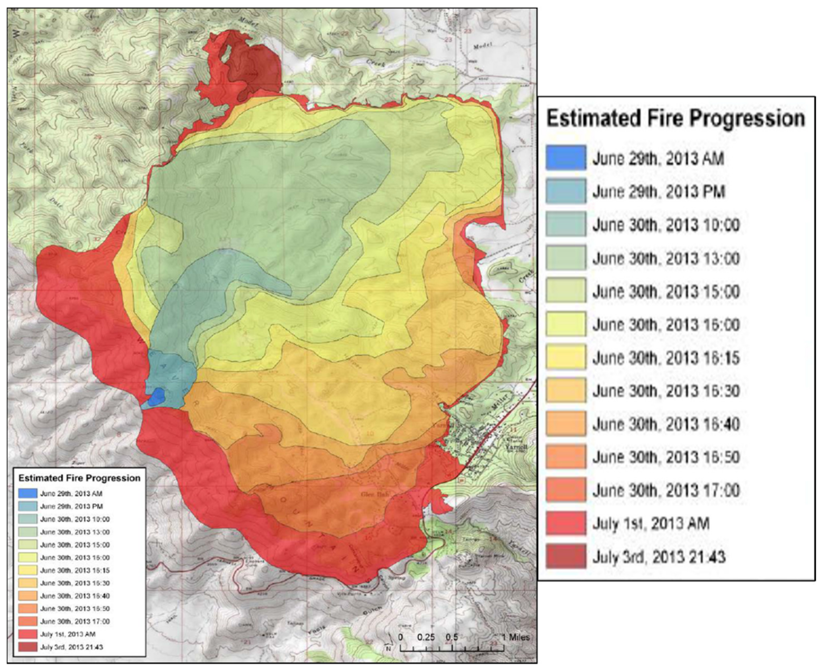
On Friday, 28 June 2013, a lightning strike from nearby convection triggered a small bush fire in west central Yavapai County, Arizona, just to the west of Yarnell, in a region known as the Yarnell Hills. A map of where Yarnell is located as shown in
Figure 1.
On Sunday, 30 June 2013, during the early afternoon hours, convection built up between Flagstaff and Prescott. By mid-afternoon, this convection had developed into a northwest-southeast oriented squall line near Dewey-Humboldt (~20 km southeast of Prescott). The squall line generated a density current, which over the next hour, raced southwestward toward Yarnell. By about 1630 MST (2330Z), the density current arrived at the Yarnell Hills region and created a sudden shift in the fire direction from moving eastward, then to the south, and then southwestward (
Figure 2 [
1]). This sudden shift in the fire direction overcame and trapped 19 firefighters (Granite Mountain hotshots) battling the flame on the western front, which led to their unfortunate demise. The fire environment at the time was exceptionally hot and dry. Fire danger was high to extreme because of extreme drought conditions during the transition to the southwest monsoon summer season. During this seasonal transition, temperatures are typically hot. The relative humidity values remain low but fluctuate as storms become more numerous. The winds are highly variable with the highest wind speeds occurring during thunderstorms. These storms can generate strong downdrafts, microbursts, outflows, and gust fronts, all of which can affect fire behavior.
Wind affects fire by removing moisture from the air, igniting new fires through firebrand transport, and increasing oxygen supply. The biggest effect of wind is on the change in fire spread direction and rate [
2] which many studies have examined [
3,
4,
5,
6,
7,
8]. Wind shifts affecting fire spread, such as in the Yarnell Hill Fire, were also observed in the Honey Fire that increased personnel risk and fire intensity [
9], and in the Bass River Fire which led to fatalities [
10]. Although not the focus in this study, synoptically induced severe downslope winds can affect fires near high elevations such as the Camp Fire [
11], Witch Fire [
12], and the Thomas Fire [
13]. The numerical modeling in these studies has had mixed results when compared to observations. In the Dude Fire, model results closely resembled the observed fire behavior, and in the Waldo Canyon Fire, the gust fronts were simulated but the timing was 2 h too early. In the burn over incident at the St. Sebastian River Preserve and in the Bass River Fire, the weather forecasts and numerical modeling did not predict the wind accurately when compared to observations. In the Camp Fire, models performed decently with some surface observations. However, non-standardized practices led to poor performance with two commercial weather stations. These studies have indicated that the unpredictability and poor understanding of fundamental dynamical processes at the complex terrain scale of local wind strength and direction makes the numerical prediction of these winds and wind surges challenging, especially on small time scales as in the Yarnell Hill Fire. Thus, it is critical to study more fires where the wind played a vital role to improve fire weather prediction, create increased public safety, and reduce loss of life and property. Previous studies involving the Yarnell Hill Fire have not focused on the role of the environmental physical processes such as the density current generation and it is strengthening/weakening. There have been studies that investigated human factors such as the chain of error [
14] and the decision-making process, communication, and dynamic flows of information, in which limitations of standard practices in the dangerous wildfire conditions were, discovered [
15]. A study from the University of Berkley has also looked at the Yarnell Fire in part to determine whether fire station infrastructure is suitably placed such that areas of the highest wildfire risk are protected using a Geographic Information Systems approach [
16].
Other studies have examined fire propagation and its complexity [
17] and developed a novel model for fire evolution [
18]. Neither study examined the thunderstorm outflow. Additional previous research on the Yarnell Hill Fire has focused on broader gust front characteristics through in situ observations with specific applications toward aviation [
19]. This study found that wind speed, relative humidity, turbulent kinetic energy, and vertical motion increased while temperature decreased as the gust front passed. However, this study did not investigate the origins of the Yarnell gust front nor how the environment enhanced the Yarnell gust front, and its implications toward the fire shift (direction and intensity).
A recent observational study of the Yarnell case [
20] analyzed the downscale organization of convection from the synoptic to meso-beta scale. However, our approach is unique because it employs model sensitivity studies at the meso-beta/gamma scale. Another study has researched cooling in a dry surface layer by looking at downdraft maximum available potential energy (DCAPE) and expanding this through a climatological analysis (seasonal and diurnal patterns) [
21]. Finally, another recent study has led to the development and implementation of a software tool that identifies and depicts convective outflow boundaries in high-resolution numerical weather prediction models to provide guidance for fire weather forecasting [
22]. For the DCAPE investigation, the focus is only on one aspect of the gust front and how it changes in the long term. For the software tool, while useful, the research does not directly investigate the outflow boundary interaction with other phenomena in complex terrain (like with the Yarnell Hill Fire) nor isolates the most important enhancement factors.
Prior research on Yarnell [
17,
18,
19,
20,
21,
22] has shown that the numerical prediction of wind surges remains challenging because of the lack of understanding of fundamental dynamical processes at the complex terrain scale. Improving the understanding of multi-scale atmospheric processes that control the motion and longevity of extreme fire events is vital. The study presented here will help answer questions such as: Which factors were the most important toward the density current generation and propagation? What impact, if any, did the isolated mountain to the southeast of Yarnell have on the density current direction and intensity? Can a fire index predict the change in the fire environment? Lastly, what role did evaporative cooling play?
Seldom has the Yarnell Hill Fire gust front, its origins, the strengthening/weakening factors, and the associated atmospheric processes been addressed in published literature. The research presented here focuses on filling this gap to better understand how the density current was organized by its environment, which includes the Yarnell Hill Fire.
A density current, or gravity current, is a region of dense fluid that moves into an environment of less dense fluid because of horizontal pressure gradient differences across a frontal surface [
23]. In some cases, this density difference has been found to be smoke-induced [
24]. There are different types of density currents that can exist depending on the environment. For example, density currents can occur with sea-breeze fronts [
25], cold fronts [
26], drylines [
27], and can also be associated with an outflow from a thunderstorm [
28,
29]. Researchers have studied thunderstorm outflow density currents in-depth and have found bore-like disturbances [
30,
31] as well as solitary waves [
32]. Others have looked at density currents in the scope of numerical modeling and have found that, for example, while shear decreases the horizontal convergence because of the downshear-propagating density current, it is nevertheless fundamental to the dynamical organization and depth of the density current [
33]. Dynamical models have also been employed focusing on the role of stably stratified flow and cooling in density current organization and motion [
34,
35].
In the sense of affecting the fire environment, a density current is fundamentally different from a severe downslope wind event such as the Santa Ana winds in California. This wind event is generated by high pressure over the southwest U.S desert that flows westward toward a low pressure off the coast of California. Santa Ana winds increase wildfire risk from the dryness and speed of the winds, which are amplified and heated by downslope adiabatic heating along the coastal mountain lee slopes [
36]. The time scale of the Santa Ana winds is on the order of days [
37] and can be predicted up to a week in advance [
38], whereas a density current is on the order of hours [
39] and can only be predicted minutes to hours in advance as it relies on the parent thunderstorm stage [
40].
In the Yarnell case, the density current moved from the northeast to the southwest into an environment with significant vertical wind direction shear. Near the fire, this created a sudden shift in wind direction and change in intensity (
Figure 2). The wind changed from moving east to south, and then southwest and increased from ~10 to ~20 ms
−1. The density current changed the direction and speed of the wind ahead of it.
Diurnal surface sensible heating is an important factor for the generation of thunderstorms over land. Significant diurnal variations can be found globally, particularly over land and during summer. Thunderstorms occur much more often during the late afternoon over land in all seasons. This is because solar radiative heating during the day on the ground generates a late-afternoon maximum of convective available potential energy (CAPE) that is favorable for late-afternoon moist convection [
41]. In July over Arizona, CAPE arises from a high moisture tongue that comes from either the Gulf of California, Mexico, or the Gulf of Mexico into the western United States, with maximum values in the late afternoon to early evening over much of the land area. The solar-driven cycle of surface pressure results in significant large-scale convergence over most of the western United States during the day, which includes Arizona. During the nighttime, the maximum thunderstorm activity occurs east of the Rockies, which is fueled by the eastward propagation of late afternoon thunderstorms generated in the west [
42]. It is hypothesized that diurnal heating (in the context of this research, referring to the diurnal heat flux) plays one of the most significant roles in the generation of the thunderstorm, and in extension the outflow/density current, that rushed through Yarnell.
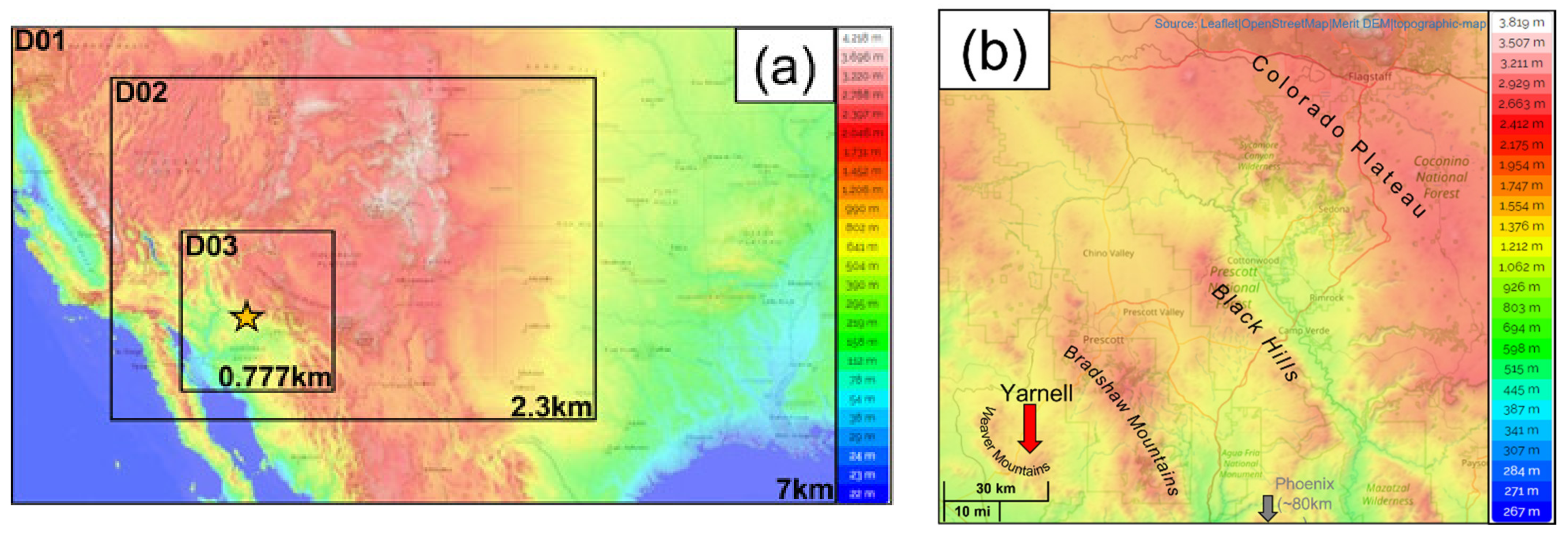
The North-Central Arizona terrain presents an excellent environment for studying atmospheric events [
43]. The terrain around the Yarnell Hills is complex, consisting of small mountains, valleys, and plateaus. The Yarnell region is elevated and Yarnell sits within a terrain “bowl”, surrounded to the west, south, and east by the Weaver Mountains. Yarnell sits at roughly 1400 m above mean sea level with the highest peak of the Weaver Mountains rising to 2000 m, creating an elevation difference of about 600 m. To the south immediately beyond the Weaver Mountains is an escarpment that drops 500 m (1400 m minus 900 m) vertically over a horizontal distance of 3500 m. Just beyond the Weaver Mountains to the east lies a northwest-southeast oriented valley at 1000 m above mean sea level. The terrain remains relatively flat toward the northeast up to the Bradshaw Mountains, and beyond lies the Verde Valley with an elevation minimum of about 1200 m. The Verde Valley borders the Black Hills to the northeast and is followed by the Mogollon Rim, which forms the southern edge of the Colorado Plateau (
Figure 1b).
Flow in and over complex terrain is multi-faceted. However, it has been found that surface flow characteristics are highly dependent on terrain slope, where the greatest difference in flow appears in regions behind the top of hills [
44]. For example, for winds with larger flow/magnitudes, forcefully channeled strong ambient wind will lead to local winds almost perpendicular to the ambient winds. For winds with smaller flow/magnitudes, thermal effects drive local winds [
45].
Additionally, thermo-topographic flows arise from differential heating [
46] and affect wind through speed-up over ridges, flow channeling in valleys, flow separation around terrain obstacles [
47], and generation of lee-side vortices parallel to mountain ridges [
48].
An isolated mountain can have different effects on the ambient wind. Thermal variations create small-scale wind circulations such as a valley breeze during the day and a mountain breeze at night [
49]. Additionally, wind increases with height and mountaintop winds are twice as high as surrounding low-altitude wind speeds [
50]. Other effects include blocking [
51] and strong downslope winds in the northern half of the lee of a ridge [
52]. It is hypothesized that the role of complex terrain may aid in the divergence and blocking of local wind.
In the following sections,
Section 2 will cover the model description and experimental design, which includes a discussion of the Hot-Dry-Windy index.
Section 3 will present the observational analysis and model validation, simulated density current generation and propagation, effects of diurnal heating and evaporative cooling, effects of complex terrain, and density current interaction.
Section 4 will conclude with a summary of the results and additional remarks including future work.
2. Model Description and Experimental Design
The Weather Research and Forecasting model version 4.0, which is also referred to as the WRF model in this study, is utilized for the numerical simulation sensitivity tests [
53]. The initial and largest domain lateral boundary conditions employ the European Centre for Medium-Range Weather Forecasts Reanalysis 5 dataset (ERA5). ERA5 is available every hour for most variables and has global coverage with a spatial resolution of approximately 30 km and 137 vertical levels from the surface up to a height of 80 km [
54]. Data are available from January 1, 1979, to the present date at the time of this writing.
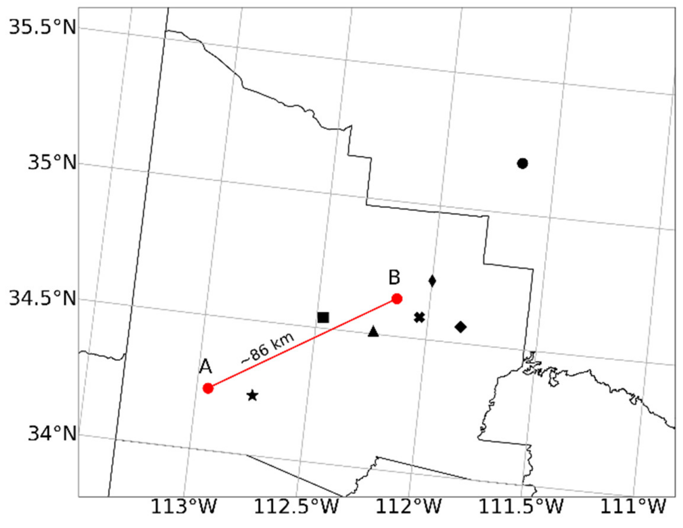
The domain was set up with a 3:1 ratio on a Lambert Conformal Map projection starting at a horizontal resolution of 7 × 7 km as the outermost domain (D01), then 2.3 × 2.3 km as domain 2 (D02), and 0.777 × 0.777 km as domain 3 (D03), as shown in
Figure 1a. D01 extends from California to Arkansas and from Wyoming to Texas. D02 extends from approximately Baja California to Central Texas and Utah to Central Texas. D03 covers most of the state of Arizona and is approximately centered over the Yarnell Hill Fire. D01 and D02 were extended toward the north and east of Arizona to capture the synoptic setup to allow for spin-up time and to capture the convection passing through the lateral boundaries. D01 starts on 29 June 2013, 1700 MST (30 June 2013, at 0000Z), and ends on 30 June 1700 MST (1 July 2013, at 0000Z), since that was when the Yarnell Hill Fire incident occurred. Each subsequent domain starts and ends on the same days but at later start times (0500 MST/1200Z for D02 and 0800 MST/1500Z for D03) and the same end time.
Table 1 summarizes the domain start/end times. For the vertical resolution, 50 stretched levels were used on all domains. Land use data are taken at 5 arcminutes (D01), 2 arcminutes (D02), and 30 arcseconds (D03) from the MODIS IGBP 21-category dataset. In meters, 5 arcminutes is about 7600 m, 2 arcminutes is about 3000 m, and 30 arcseconds is about 760 m, for a latitude of 34.22° N (Yarnell, AZ, USA). Output is written every 4 h (D01), 1 h (D02), and 15 min (D03).
The most important reason to employ the WRF with initialized, complete three-dimensional atmospheric structure is that the space-time continuity of the density current and supporting convection are resolved. Idealized modeling would likely miss key details of the horizontal variation of convection and its effects on density current organization and motion. Higher resolution simulations would benefit from employing the LES formulation to better resolve the structure of planetary boundary layer eddies that affect convective initiation and maintenance in the complex terrain.
Four simulations including three sensitivity tests were conducted to examine the density current generation, propagation, and interaction through the complex terrain. Initially, a control case (CNTL) was run for comparison, then the southeast Weaver Mountain (NSEM) was removed to study the blocking effects. Afterward, evaporative cooling was turned off (NEVP) to investigate the importance of latent heat change effects. Finally, the last sensitivity test involved turning off the diurnal surface sensible heating to examine the importance of convective instability building during the day (NDHT).
For the CNTL case, the microphysics used was the Purdue Lin scheme [
55]. For the surface, land-surface, and boundary layer physics schemes, the physics parameterizations were set to the Eta Similarity scheme [
56,
57,
58,
59], unified Noah land-surface model [
60], and Mellor–Yamada–Janjic (Eta) TKE [
57,
61]. The cumulus parameterization was set to the Grell–Freitas ensemble scheme [
62] only for the outermost domain (D01) since this scheme is scale sensitive for a horizontal domain resolution of 7 km. For all other domains, no cumulus parameterization scheme was used. These schemes are summarized in
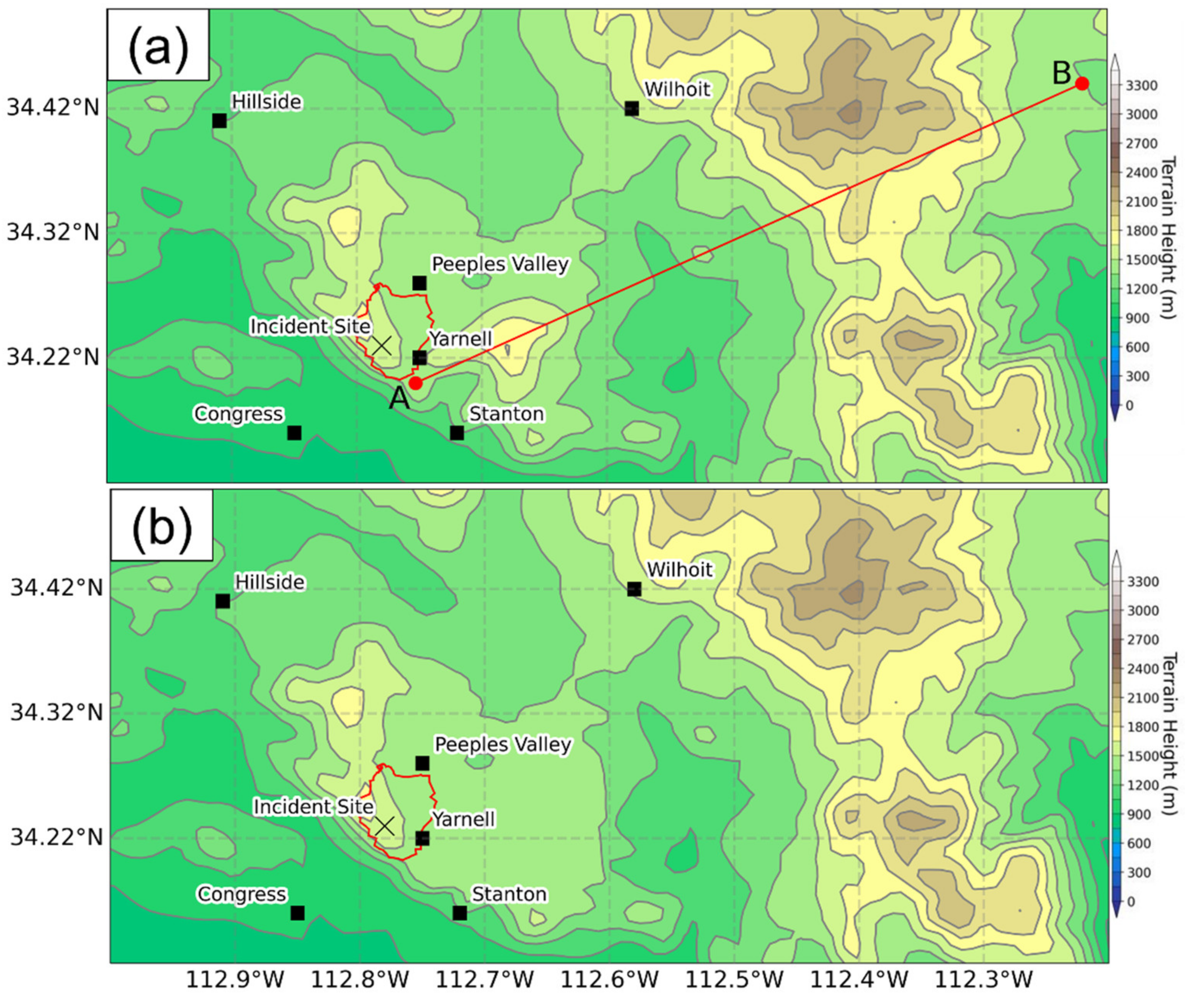
Table 2. These physics, in general, were chosen to include parameterizations that are not too computationally expensive but still representative for the convection and the wind event. The Purdue–Lin scheme was chosen because it is a five-class microphysics scheme that includes graupel and because of its ability to handle high-resolution domains. The Eta Similarity scheme was chosen because of the choice for the boundary layer physics scheme (paired), the unified Noah land-surface model because of its sophisticated vegetation modeling, and the Mellor–Yamada–Janjic (Eta) TKE scheme for its ability to handle thin layers. In the NSEM case, the only change was flattening the terrain of the isolated Weaver Mountain to that of the surrounding terrain (
Figure 3b). For the NEVP case, the evaporative cooling was turned off in the Lin microphysics module (to turn off the reset of potential temperature) and within the moist physics subroutine in the long time step utility code. Finally, for the NDHT case, the surface layer and boundary layer physics schemes were turned off. The following sections will focus on the results from D03, not from the ERA5 reanalysis, which is the initializing dataset.
The Hot-Dry-Windy (HDW) Index
Historically, fire prediction has been formulated with the lower atmosphere severity index, also called the Haines Index [
63]. The Haines Index is a fire index that computes the potential for wildfire based on the sum of a stability and a dryness term on a scale of 1–6. There are three variants of the Haines Index, a low, medium, and high variant. Despite its popularity, the Haines Index has been found to be problematic because it does not account for the wind factor which is often vital to any wildfire growth [
64]. A new index, the one used in this study, has recently been formulated called the Hot-Dry-Windy Index (HDW) that predicts the potential for fire using temperature, moisture, and wind, three parameters that are much more relevant to wildfire spread and growth [
65]. Srock et al. (2018) describe an operational variant of the HDW called the HDWI as well, where the “I” stands for index. The HDWI uses the Climate Forecast System Reanalysis (CFSR) as input data, which are provided at a lower spatial and temporal resolution than the ERA-5 dataset. Because of the lower resolutions, HDWI, as discussed in Srock et al. (2018), is not appropriate for predicting fine-scale weather (such as density currents) to affect fire behavior. Here, HDW is presented from the raw formulation rather than from the operational variant (HDWI) and for some theory and background. HDW Equation (1) is defined as per below:
In Equation (1), HDW is the product of the horizontal wind (U) and the vapor pressure deficiency (VPD) as a function of the temperature (T) in Kelvin and the mixing ratio (q). The VPD Equation (2) is the difference between the saturated vapor pressure () and the vapor pressure (), where and are measured in hectopascals (hPa). To obtain the saturated vapor pressure, the Clausius–Clapeyron Equation (3) can be used. Here, and are the latent heat of vaporization at 0 °C and the gas constant for water vapor and have constant values of 2.5 × 10⁶ J kg−1 and 461 J K−1 kg−1, respectively. To obtain the vapor pressure, the relative humidity (RH) is multiplied by the saturated vapor pressure, Equation (4). HDW is measured in hundreds and is nondimensional, where 100 is low and 800 is considered high. The interpolation of HDW is performed at 830 hPa as this level is closest to the ground without intersecting the ground (or a significant portion of mountains).
HDW has been proven effective for fires such as the Pagami Fire where HDW identified the specific day on which the fire was most difficult to manage, the Bastrop Fire where HDW identified days where an initiating fire may spread rapidly because of large-scale weather conditions, and the Double Trouble Fire where HDW identified days where fires can become difficult to manage [
65]. Climatologically, HDW provides insight into near-surface climatic conditions which can be used to determine temperature and humidity trends related to climate classification systems [
66]. This study will also attempt to examine the fire predictability for the Yarnell Hill Fire using HDW, not the HDWI formulation.
3. Results
This section will begin with an analysis of the general environment and radar for 30 June 2013, the day of the Yarnell Hill Fire incident, and a comparison to the CNTL case with justification. Afterward, an explanation of the initial density current generation and propagation will be presented. Then, an analysis of the NDHT, NEVP, and NSEM cases. The section will finish with an overview of HDW during the event for the CNTL simulation and a comparison to observations at Peeples Valley and Stanton, AZ, USA (employed to calculate HDW). Finally, a comparison will be performed between the simulated wind magnitude, wind direction, and the simulated relative humidity for the CNTL case, and the observed surface wind magnitude, wind direction, and relative humidity at Cherry, Peeples Valley, and Stanton, AZ, USA.
3.1. Observational Analysis and Model Validation
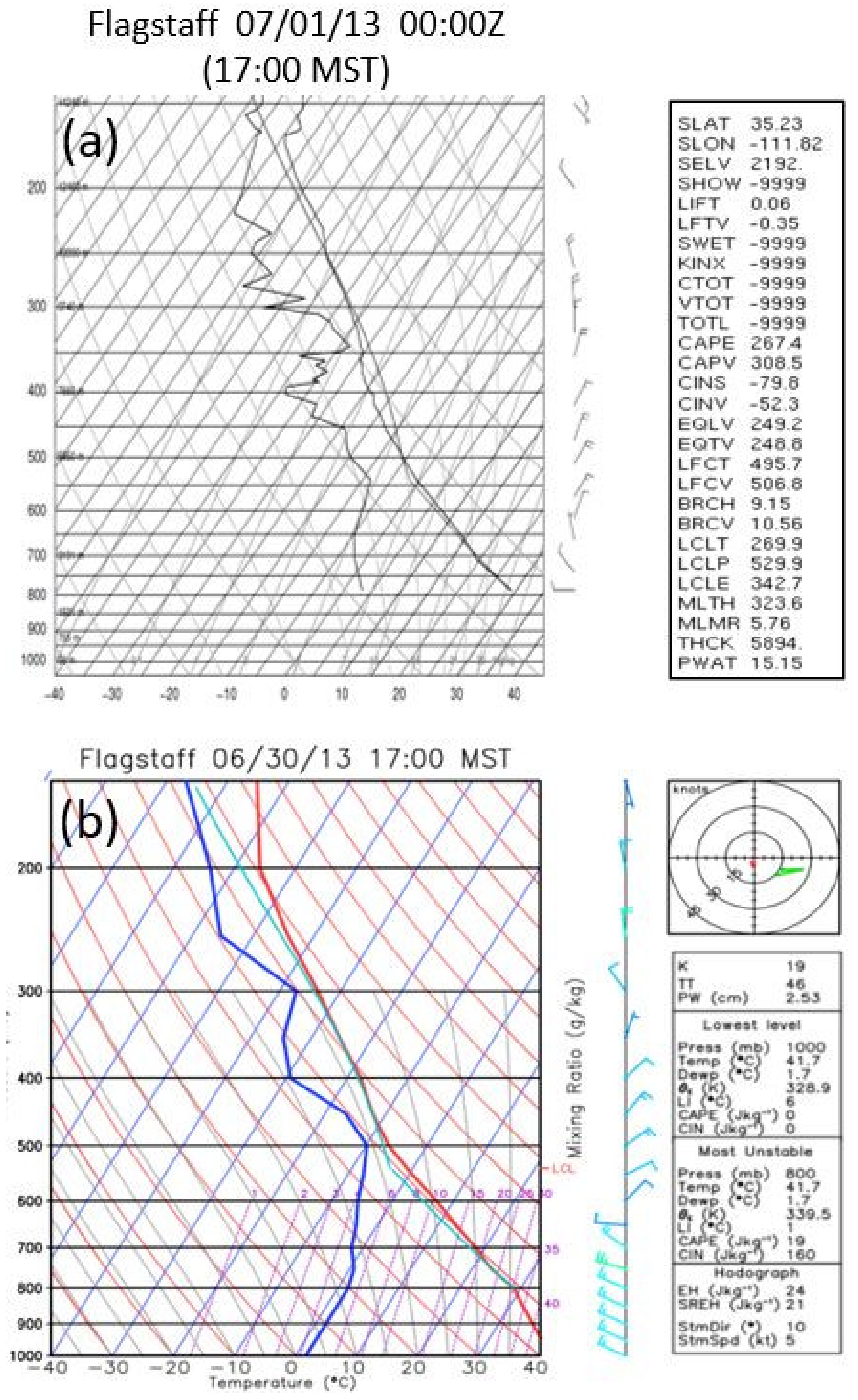
Figure 4 shows the observed and simulated soundings for the CNTL case at Flagstaff on 06/30/13 at 1700 MST (07/01/13, at 0000Z). The surface temperatures and dew points are in general agreement and show as approximately 25 and 2 °C, respectively. In the mid-troposphere, the soundings are in some disagreement. Specifically, the simulated sounding shows a slightly more saturated environment. Similarly, in the upper troposphere, the inversion found in the observed sounding is smaller than in the simulated sounding. Winds were also generally in agreement throughout the sounding. Overall, the soundings are similar and thus the simulation is representative of the observed environment.
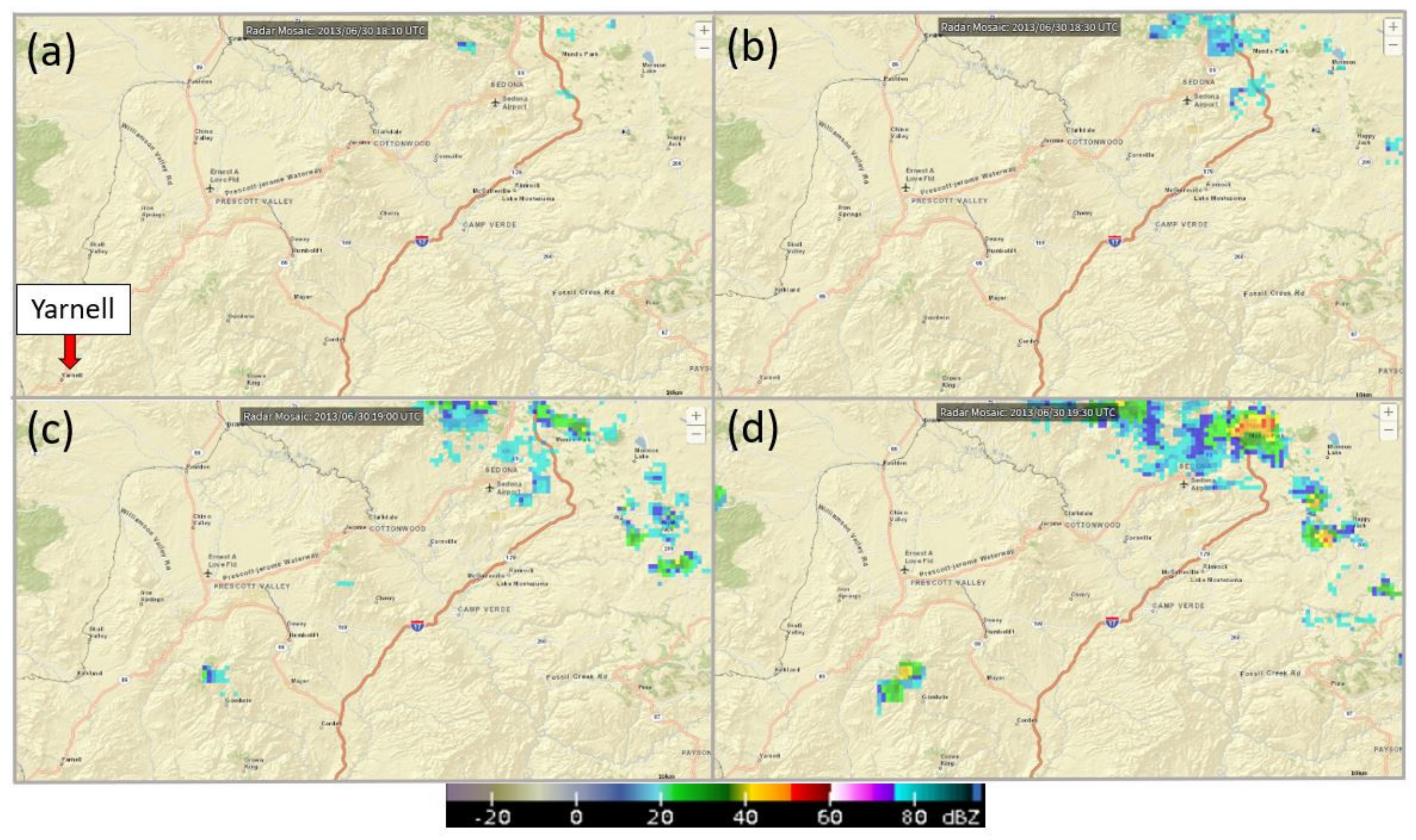
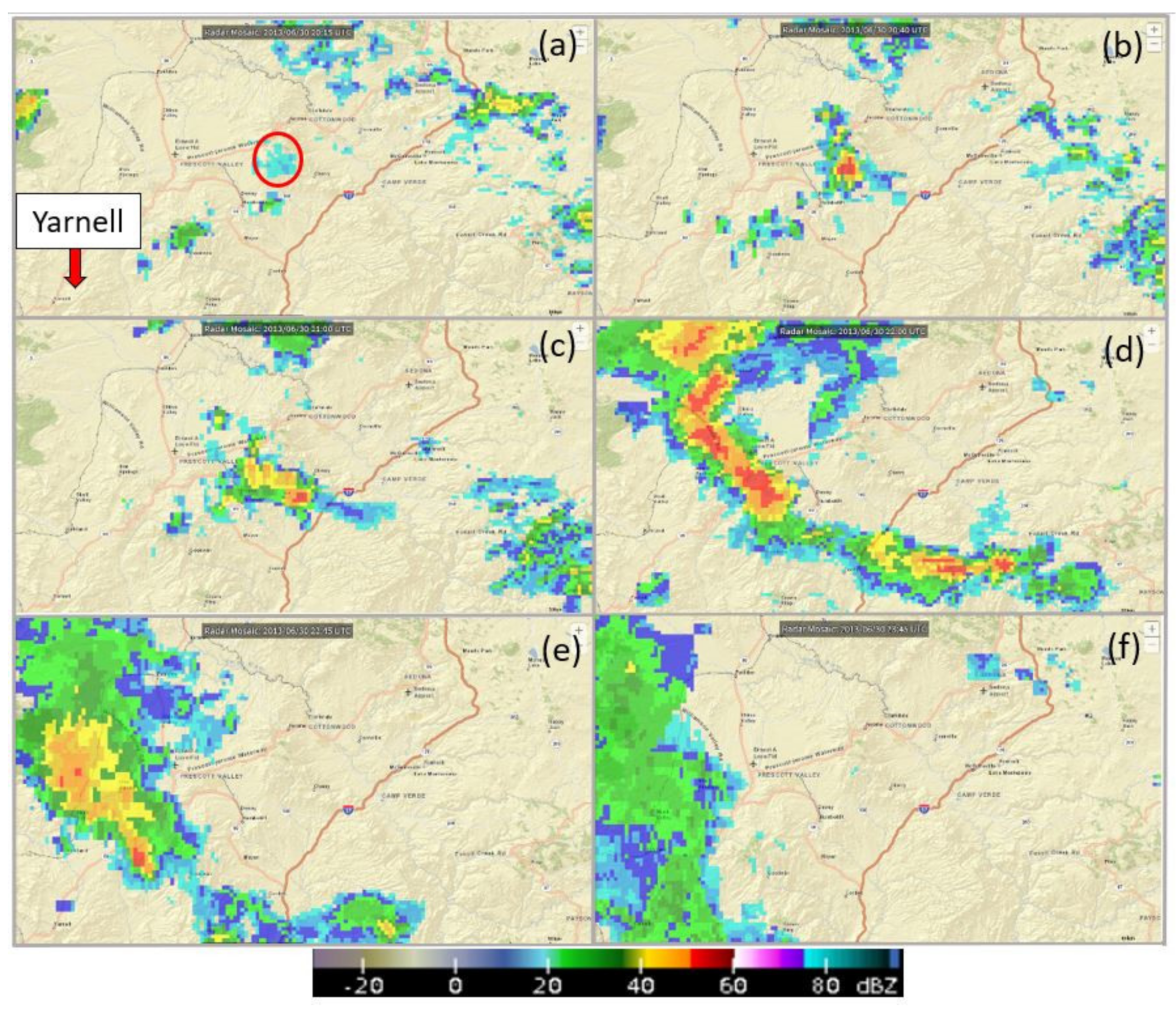
During the morning and early afternoon hours on 30 June 2013, there was scattered, generally unorganized, and localized convection over the center-west portion of Arizona, stretching from Yarnell to just southwest of Sedona with a focus near Sedona (
Figure 5). Throughout the afternoon (
Figure 6), the environment became more conducive to organized convection as temperatures began to rise and moisture was transported from the east and north. Both
Figure 5 and
Figure 6 show the reflectivity mosaic from NCEI on 30 June. By 1315 MST/2015Z, a small cell (
Figure 6a, red circle) had developed west of Cherry, AZ, USA (by the Black Hills (note
Figure 1)) and North of Dewey, AZ, USA. This served as the anchor point for later convection resulting from the air that was likely lifted by the Mountain–Plains Solenoid (MPS) circulation over the Black Hills that created the first ensemble of density currents. The cell remained relatively stationary and reached its maximum reflectivity (~50 dBZ) within 25 min. By 1400 MST (2100Z), a small-scale squall line had developed around the periphery, oriented northwest to southeast from Prescott Valley to just east of Interstate 17, and began to propagate toward the southwest. By 1500 MST, the squall line rapidly intensified as convection fired along the northwest and southeast sides stretching from Paulden, AZ, USA, to Pine, AZ, USA. The environment toward the northwest remained favorable for convection while the environment toward the center of the squall line remained less conducive to convection. By 1545 MST (2245Z), the squall line had become wider toward the northwest and began its transition past peak intensity and into stratiform precipitation. By 1645 MST, the entire system has transitioned to stratiform precipitation as it moved over the Yarnell Hill area.
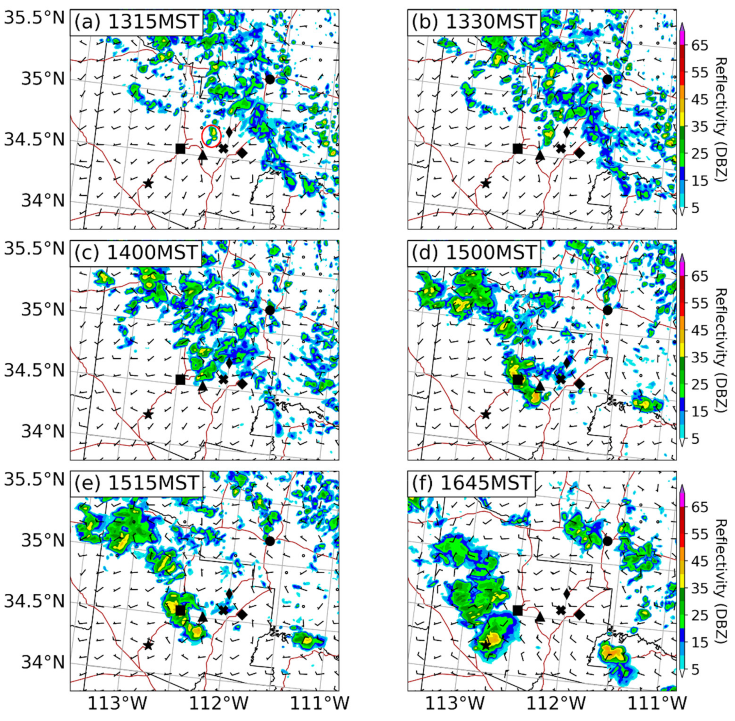
Comparing the observed radar to the CNTL case shows that the simulation is similar in convective structure, timing, and location (
Figure 7). In the CNTL case, by 1315 MST, there is convection toward the northeastern part of the domain, which is slightly more widespread than in the observations, with the convection extending slightly further toward the northwest and southeast. The squall line begins around the same time (1315 MST) and place (west of Cherry and north of Dewey-Humboldt) but is significantly stronger in the simulation. The squall line fully developed similarly in the simulation to the observed radar, at 1500 MST. However, the simulated squall line appears to be more northwest biased and does not initiate toward the south and east of Yarnell as in the observations. A transition into stratiform precipitation is seen later toward the end of the simulation starting at 1645 MST. Overall, the convection initialization and location for the analysis are generally in agreement but the buildup and break down time to maximum intensity and stratiform precipitation, respectively, take longer to reach in the CNTL simulation. Comparing the reflectivity at 1315 MST, 5 dBZ is depicted in the observed vs. nearly 40 dBZ in the simulation at the location where the squall line develops. About 30 min later, 50 dBZ is depicted in the observations vs. nearly 40 dBZ in the simulation, which is more inline. Since the CNTL case and the observations are generally in agreement, the analysis was conducted based on the input parameters from the CNTL case and the simulation modifications made where appropriate and are described more lately. It should be noted that, in the observations, the nearest weather radar is Flagstaff (KFLX), which is about 150 km toward the northeast, outside of the domain. The simulation depicts the maximum vertical column reflectivity, thus what the radar sees may not necessarily be the maximum reflectivity in the vertical column because of the beam angle by the time it reaches Yavapai County.
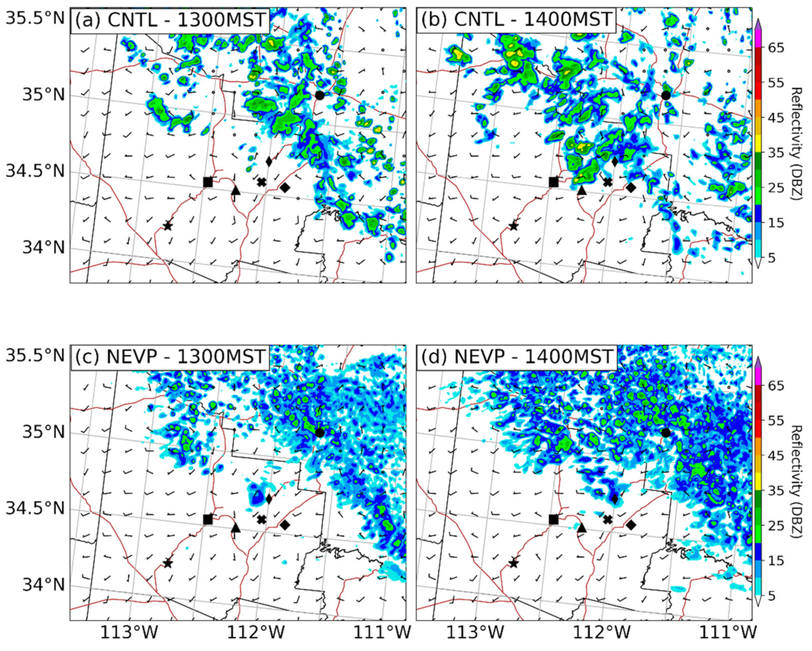
Figure 8 shows the simulated reflectivity between the CNTL and NEVP cases. From before, the CNTL case (a-b) agrees rather well with the observed reflectivity. In the simulation, the convection that initialized over the Black Hills is present but slightly further toward the north by 1300 MST (2000Z). By 1400 MST, the convection develops into a small squall line that is oriented northwest to the southeast that propagates southwestwards where the intensity is slightly less than what was observed. For the NEVP case, the convection initialization over the Black Hills is also seen at 1300 MST with a slight offset toward the north. However, the convection remains stationary and does not intensify by 1400 MST. In the NDHT case (not shown), little/no convection is present in either time since there is no surface sensible heating. There is only a small patch of extremely localized weak convection toward the eastern part of the domain, which results from other diabatic heating processes.
The Yarnell Hill environment on 30 June 2013 was exceptionally hot and dry with temperatures near 100 degrees Fahrenheit and relative humidity below 30% (in most cases, well below).
Table 3 shows the surface observations at Cherry, Peeples Valley (about 6 km to the north-northwest of Yarnell), and Stanton, AZ, USA (about 6 km to the southeast of Yarnell). The squall line that generated the density current that rushed through the Yarnell Hill Fire developed to the southwest of Cherry and propagated southwestward. The observed wind surge in Cherry is a weaker component of the density current that propagated northeastward. The portion of the density current toward the southwest propagated first through Peeples Valley at a velocity of nearly 8 ms
−1 during the late afternoon and then through Yarnell and Stanton shortly after at a velocity of nearly 13 ms
−1, according to the observed data. The passage of the density current is noted by an increase in wind speed, shift in wind direction, drop in temperatures, and an increase in relative humidity. How the simulated results compared to the observations will be evaluated at the end of this section. The next subsection will explore the density current and the role of the MPS, which explains the location and intensity of the convection over the Black Hills.
3.2. Simulated Density Current Generation and Propagation
Since the convection propagation was from the northeast toward the southwest on 30 June 2013, a cross-section parallel to this direction can be defined. Cross-section H (
Figure 9) is used and extends just west-southwest of Yarnell, AZ, USA, northeastwards to the Black Hills. For the MPS discussion, the cross-section is extended by about 20 km to the northeast to cover more of the Black Hills.
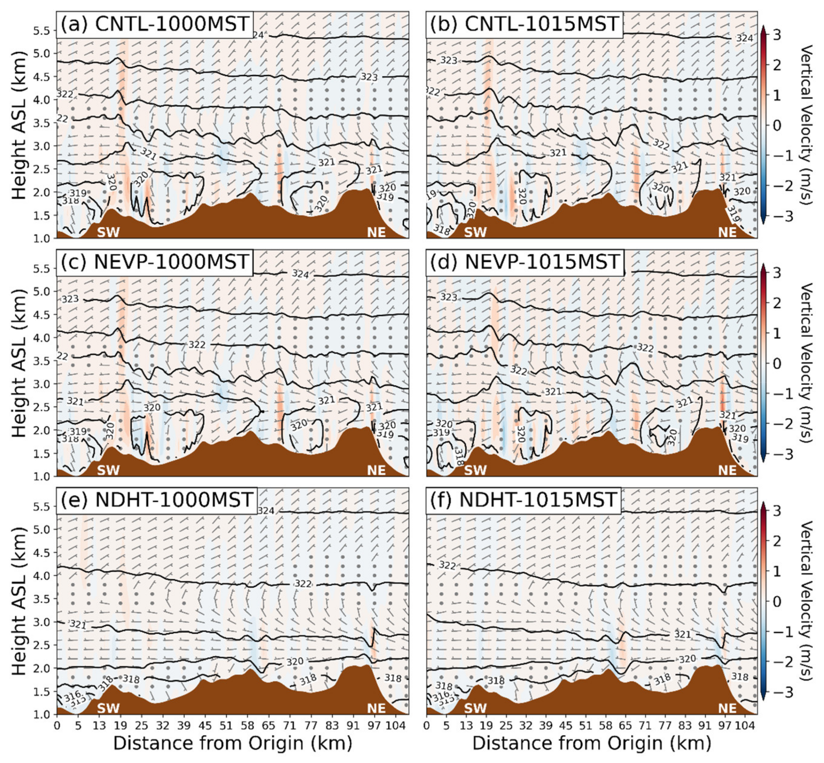
The formation of the density current is initialized from convection over the Black Hills. This convection is triggered by an MPS circulation that develops during the late morning in the CNTL simulation (
Figure 10). From the left column of
Figure 10 (panels a, c, and e), around 1000 MST, a cold pocket is present on the lee side of the Black Hills which is seen from the expanded isentropes. The cold pocket reaches from the bottom of the Verde Valley to the peak of the Black Hills in the cross-section. The origin of the cold pocket arises from a katabatic jet flow down the northeastern slope accompanying a nocturnal jet. When the sun rises, this nocturnal jet begins to slow which produces convergence that lifts the cold air, creating a stable core. After sunrise, the nocturnal katabatic flow is replaced by a mesoscale solenoidal circulation, in this case by 1000 MST, which is seen by the faint up/down vertical velocity couplet anchored to the lee slope. Upslope flow is produced from the horizontal pressure gradient force toward the slope because of the buoyancy associated with the surface sensible heating. The main upward flow is in a narrow zone above the slope, known as the leeside convergence zone (LCZ). The LCZ acts to lift air, which creates a cold core (upward kink in isentropes on the lee slope of Black Hills). This lifted air advects additional moisture into the atmosphere that provides the fuel for the convection that forms in the early afternoon which subsequently generates the density current resulting from evaporative cooling by the precipitation downdraft.
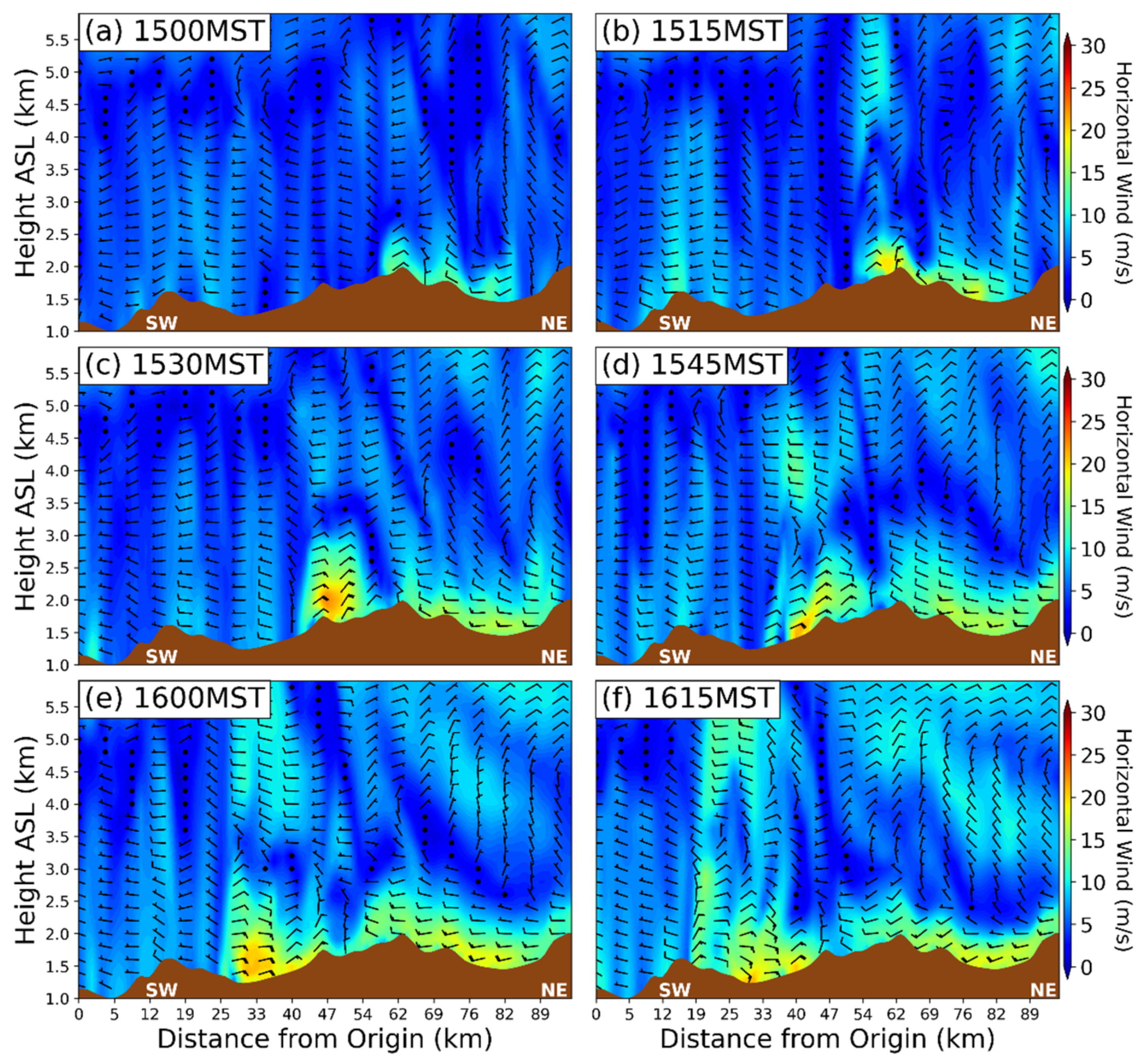
During the initiation of convection in the early afternoon, the density current (henceforth denoted as D0) propagated southwestwards from the Mogollon Rim through the Verde Valley and approached the Black Hills. D0 encountered the region of MPS-initiated convection developing southeastwards along the Black Hills. The convection strengthened and radiated three additional density currents that emanated around the periphery of the Black Hills, denoted D1a, D1b, and D1c. D1a propagated northeastwards back toward the northwestern Verde Valley, D1b intensifies in the Verde Valley and southeast side of the Black Hills with significant momentum as cold air flowed down the Black Hills southeastern side, and D1c developed on the leeside of the Black Hills and propagated southwestwards first toward the Bradshaw Mountains and then toward Peeples Valley and Yarnell. The heating above the Black Hills and northeasterly flow from D0 in the Verde Valley were catalysts for the convection. In the CNTL case (
Figure 11), the formation of a density current begins by 1500 MST near the Black Hills to the northeast. D1c propagated toward and flowed over the Bradshaw Mountains, where the model downscaled into another density current after the convective outflow moved over the region centered on Mount Union (near 34.4° N, 112.4° W) around 1515 MST (2215Z). Here, the density current cloud line was virtually centered on Mount Union near the crest of the Bradshaw Mountains above 7900 feet MSL. Acceleration of its motion occurs on the lee slopes to about 14.4 ms
−1 [(54 − 42) km/(15 min × 60 s/min)] and by 1530 MST it increased to a magnitude of about 22 ms
−1. By 1600 MST, the density current began to slow down as it reached the base of the Bradshaw Mountains and approached the Yarnell area. However, the magnitude remained at nearly its strongest value of 20 ms
−1 as it approached Peeples Valley, Stanton, and finally Yarnell (
Figure 12). The wind surge moved rapidly through Yarnell, over and down the lee side of the Weaver Mountains, from 1600 to 1630 MST. A second momentum surge at 1645 MST rushed through Yarnell as well. The combination of these two surges rapidly shifted the fire motion from moving east to south and then southwest, trapping the 19 firefighters. The surges are examined further in
Section 3.4.
The MPS-initiated convection builds from the Black Hills over Prescott Valley and then maintains enough continuity over the Bradshaw Mountains to create a distinct line with the help of the downslope forcing of its outflow. Upslope flow around the Weaver Mountains triggered weak convection that rapidly stratiformed-out while the northeasterly flow from D1c (evident most strongly at Stanton) accelerated through the firefighter’s location. The outflow boundary originating from a line of thunderstorms to the north-northeast swept over the fire area approximately between 1618 and 1630 MST. The outflow boundary moved from north to south affecting the fire area near Peeples Valley first. The effect on the fire was immediate and significant. The primary fire spread direction was forced to make a rapid south-southwesterly shift toward the firefighters’ location; fire intensities and resulting flame lengths doubled while rates of spread tripled. What had been problematic fire behavior became extremely dangerous.
3.3. Effects of Diurnal Heating and Evaporative Cooling
Based on the factors studied, diurnal surface sensible heating was the second-most important factor for modifying the density current generation and propagation dynamics in time moving southwestward from the Black Hills. The Black Hills’ MPS signature is opposite to the other cases and weak for the NDHT case shown in
Figure 10e,f. When the diurnal heating is turned off, no surface sensible heating is present. Without any surface sensible heating, no buoyancy is present, the horizontal pressure gradient is reduced, and upslope flow (which is a critical feature to the MPS circulation) is reduced/removed. The organizing mechanism for the MPS is turned off and moist convection is suppressed over the Black Hills. A density current is not generated since there is no moist convection that would create the evaporative cooling needed for the density current formation. The MPS-like signature does not evolve past the transitional stage into the developing stage in which flow fully reverses from downslope to upslope, which would be conducive for convection. Thus, an MPS solenoidal circulation is not seen.
The environment without diurnal surface sensible heating (NDHT) generates no simulated reflectivity and little to no vertical velocity (not shown). The potential temperature remains constant as well near the surface at 312 K at 1.5 km above ground level (AGL), increasing to 320 K by 2.5 km AGL. The relative humidity within the first 2 km AGL is between 30 and 40% and drops to 20–30% from 2 to 3.5 km, thus further indicating the environmental uniformity. The horizontal wind near the surface was seen to be from the south, averaging 5 ms−1 and reaching a maximum of 15 ms−1 in the valley southwest of Yarnell. The horizontal wind transitions from being from the north-northwest just above the surface, averaging 5–10 ms−1 and reaching a maximum of 10 ms−1 above the lee slope of the Bradshaw Mountains, to being from the east-northeast aloft, averaging 5 ms−1 with no clear maximum throughout the time frame.
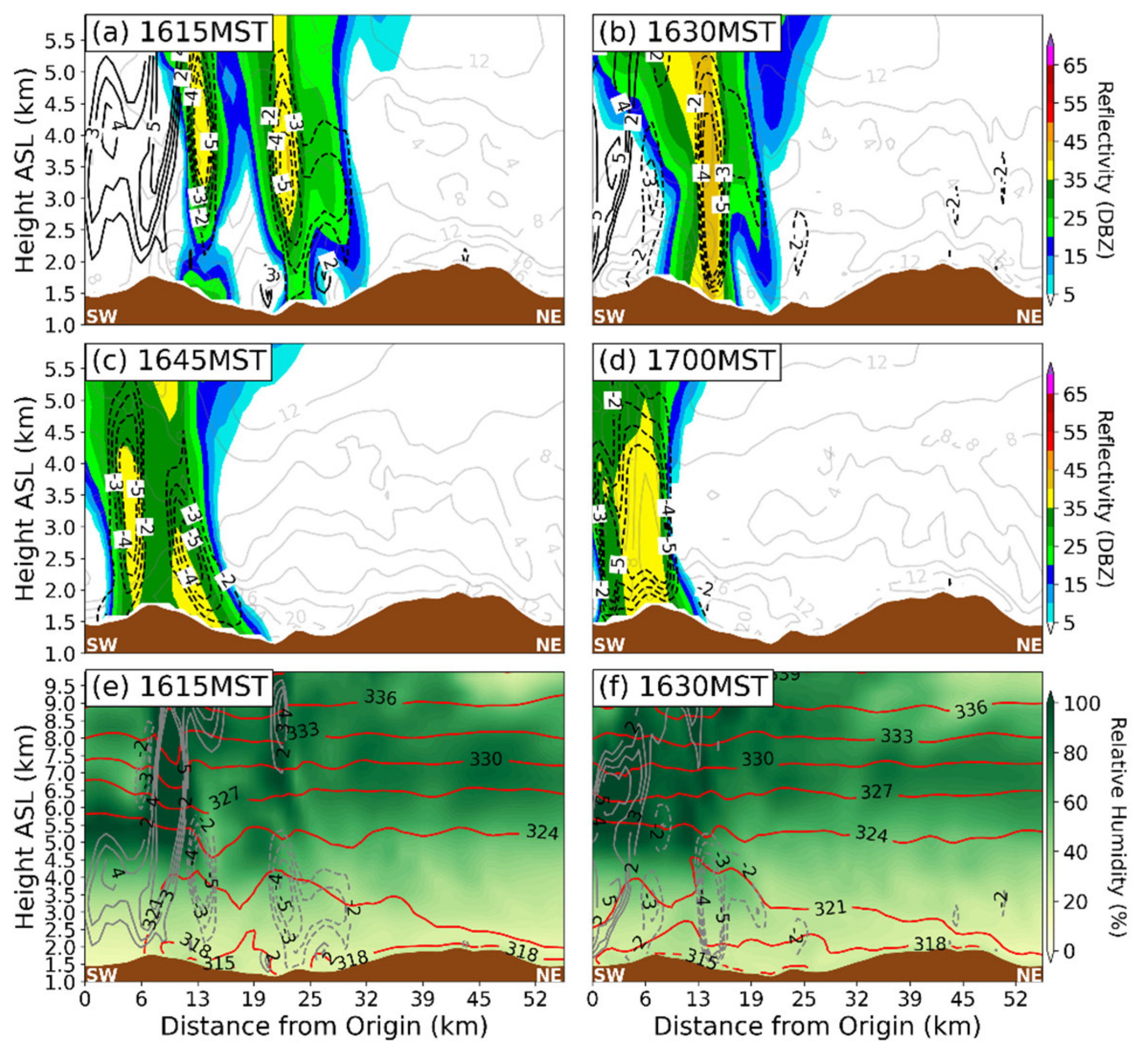
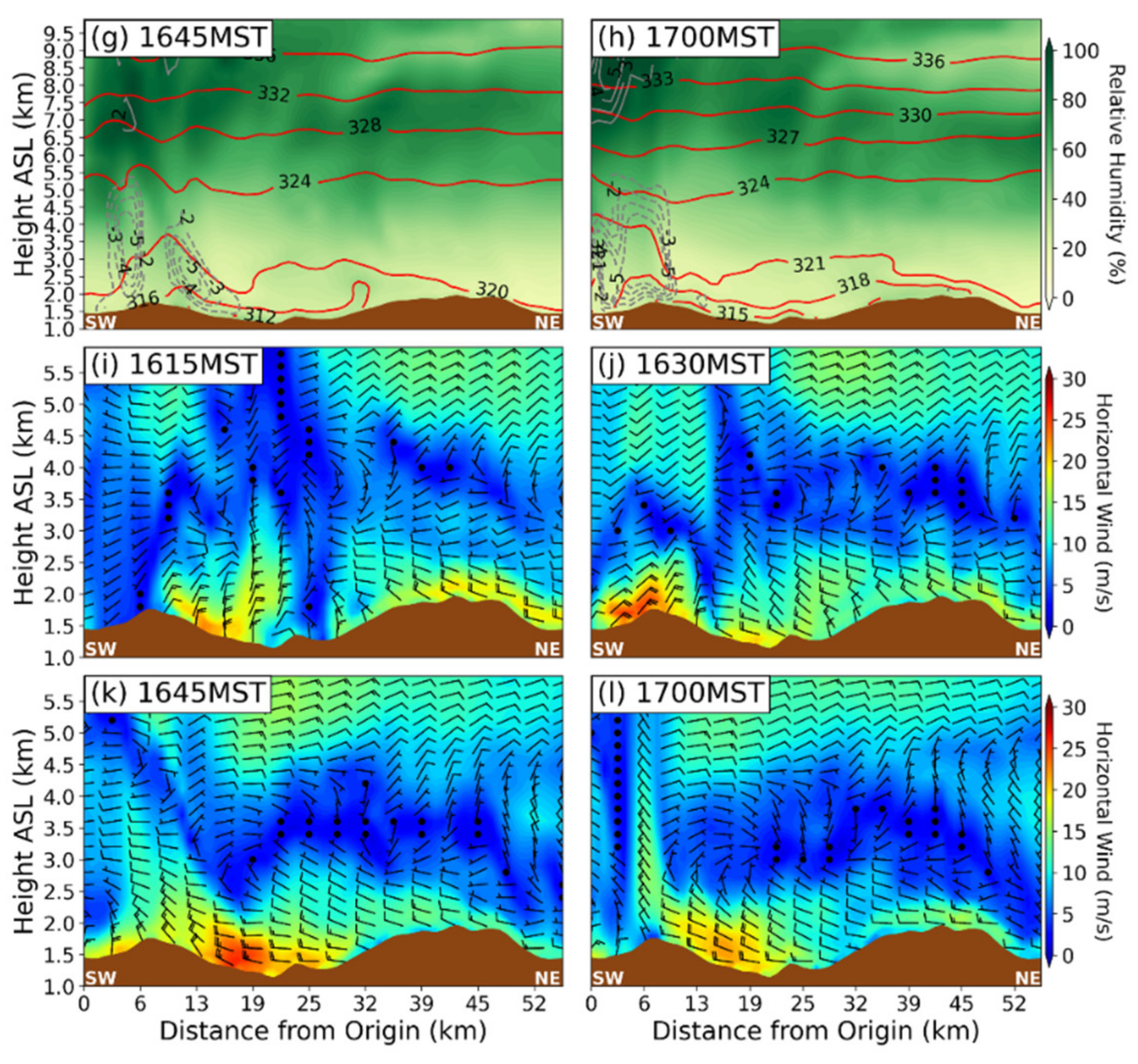
The evaporative cooling (generated by the evaporation of precipitation from the storm) played a role in initializing the density current and, to a lesser extent, the convection. This arises from the generation of a cold pool, which then initialized more convection. Thus, by turning off the evaporative cooling, no subsequent convection is initialized. From
Figure 10c,d, when evaporative cooling (NEVP) is turned off, the MPS signature is still present. Just as in the CNTL case, the MPS develops during the late morning around 1000 MST. A cold pocket also develops on the lee side of the Black Hills which is seen from the isentropic expansion. The cold pocket has a similar extent, reaching from the bottom of the Verde Valley to the peak of the Black Hills. After sunrise, the nocturnal katabatic flow begins to be replaced by the mesoscale solenoidal circulation, in this case by 1000 MST. Upslope flow is produced from the horizontal pressure gradient force toward the slope with the main upward flow in the LCZ. The MPS lifts moisture which cools and forms clouds over the Black Hills. However, any convection remains constrained far above the surface (~5 km) since the evaporative cooling process cannot act to moisten and cool the lower levels for the precipitation (and cool air) to reach the surface. Thus, no convective downburst or density current is generated.
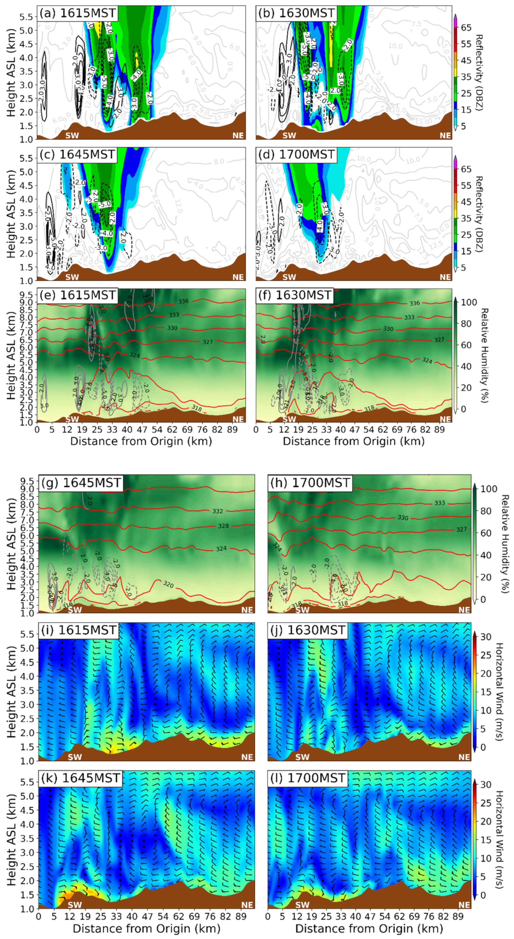
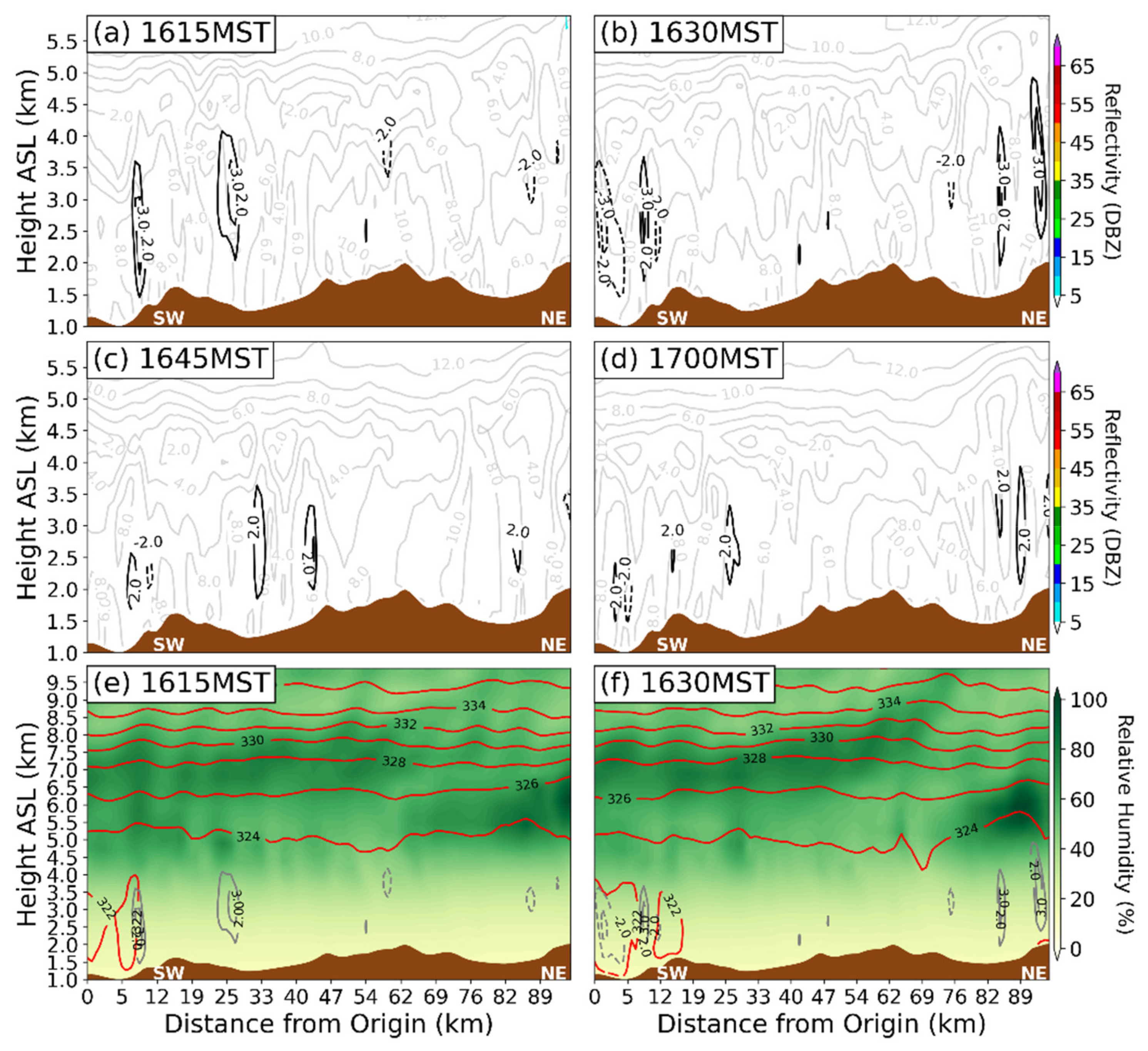
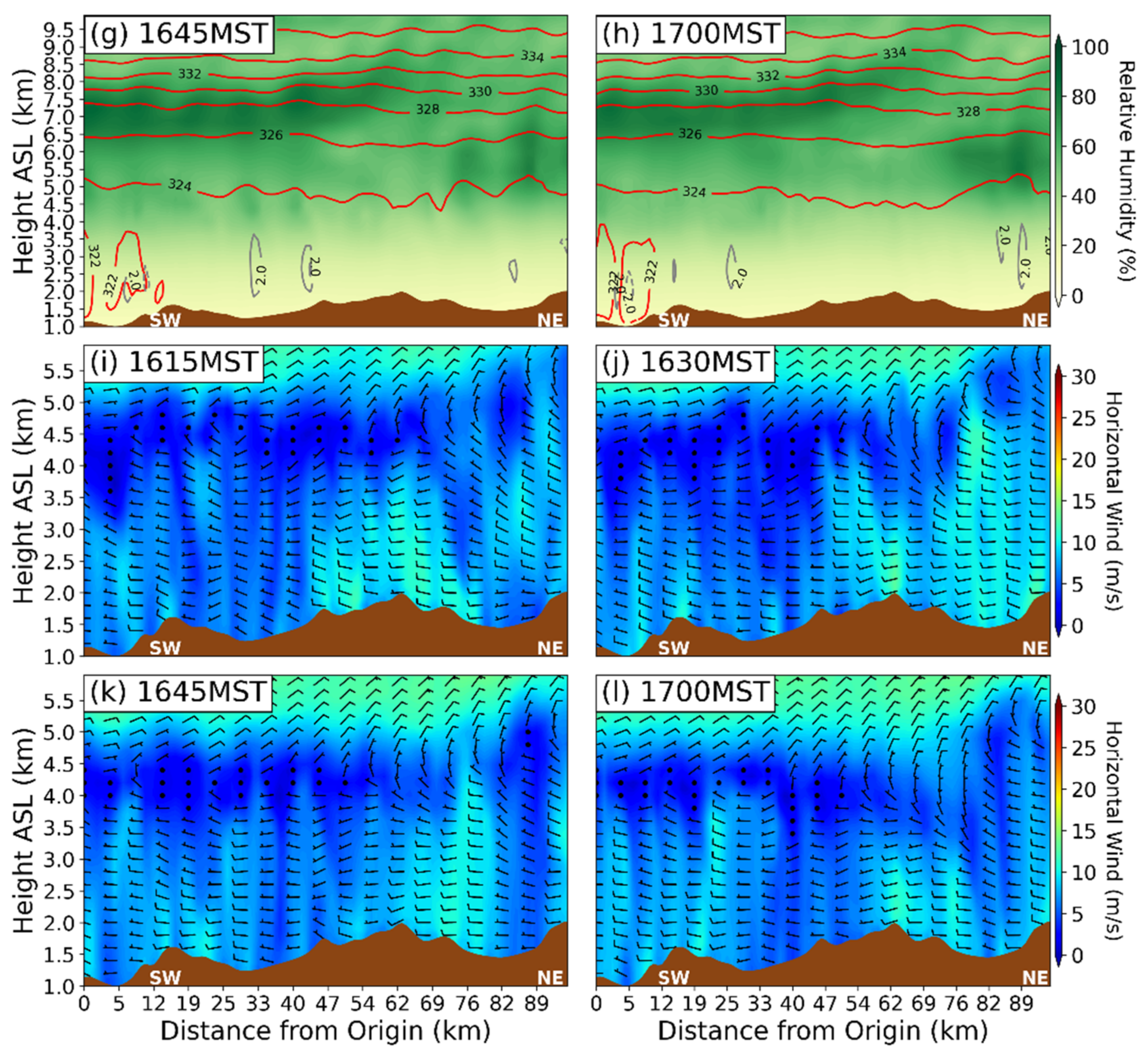
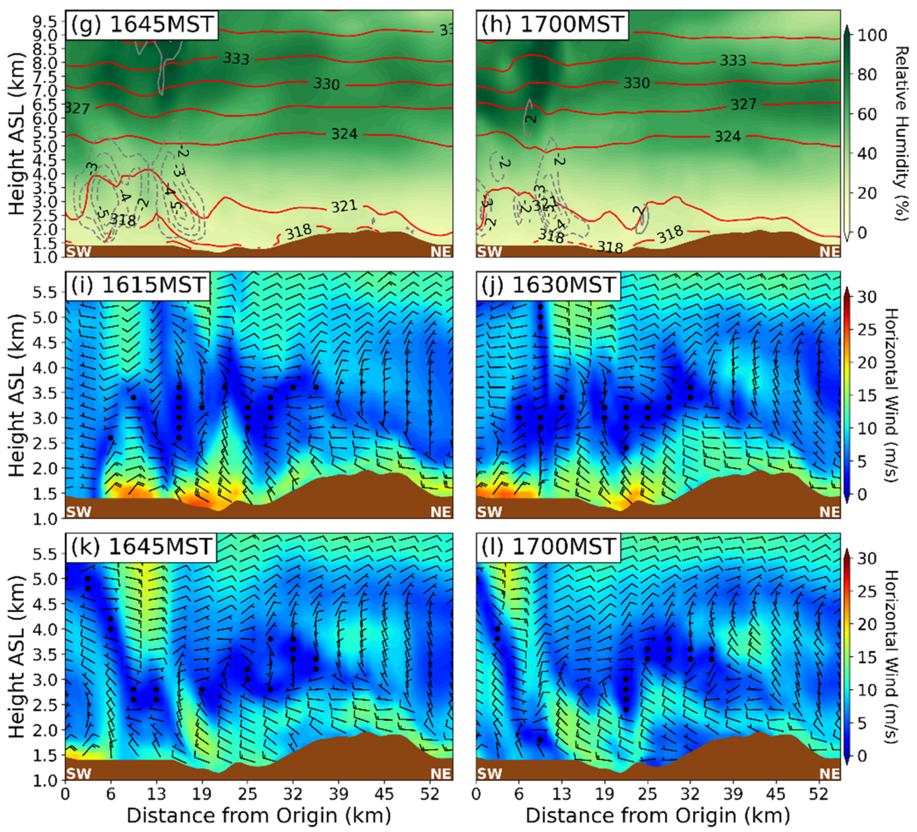
Figure 13 shows the simulated reflectivity and horizontal wind and w, theta and relative humidity and w, and horizontal wind from 1615 to 1700 MST for the NEVP case. During this time frame, no density current is generated. However, vertical motion is still present, unlike in the NDHT case. The horizontal wind is also stronger, reaching a maximum just above the surface near the peak of the Bradshaw Mountains by 1630 MST. At 6 km AGL, the horizontal wind is consistently stronger than in the NDHT case. Wind direction is slightly less uniform than in the NDHT case, which results from a repressed vertical velocity, but more uniform than in the CNTL case because of the lack of the density current. Similar conclusions can be reached for the potential temperature. When comparing the relative humidity and simulated reflectivity between cases to the CNTL case, the relative humidity is more uniform at 3 km and higher for the NEVP case and even more so for the NDHT case. The simulated reflectivity is vastly different in both the NEVP and NDHT cases compared to the CNTL case.
3.4. Effects of Complex Terrain
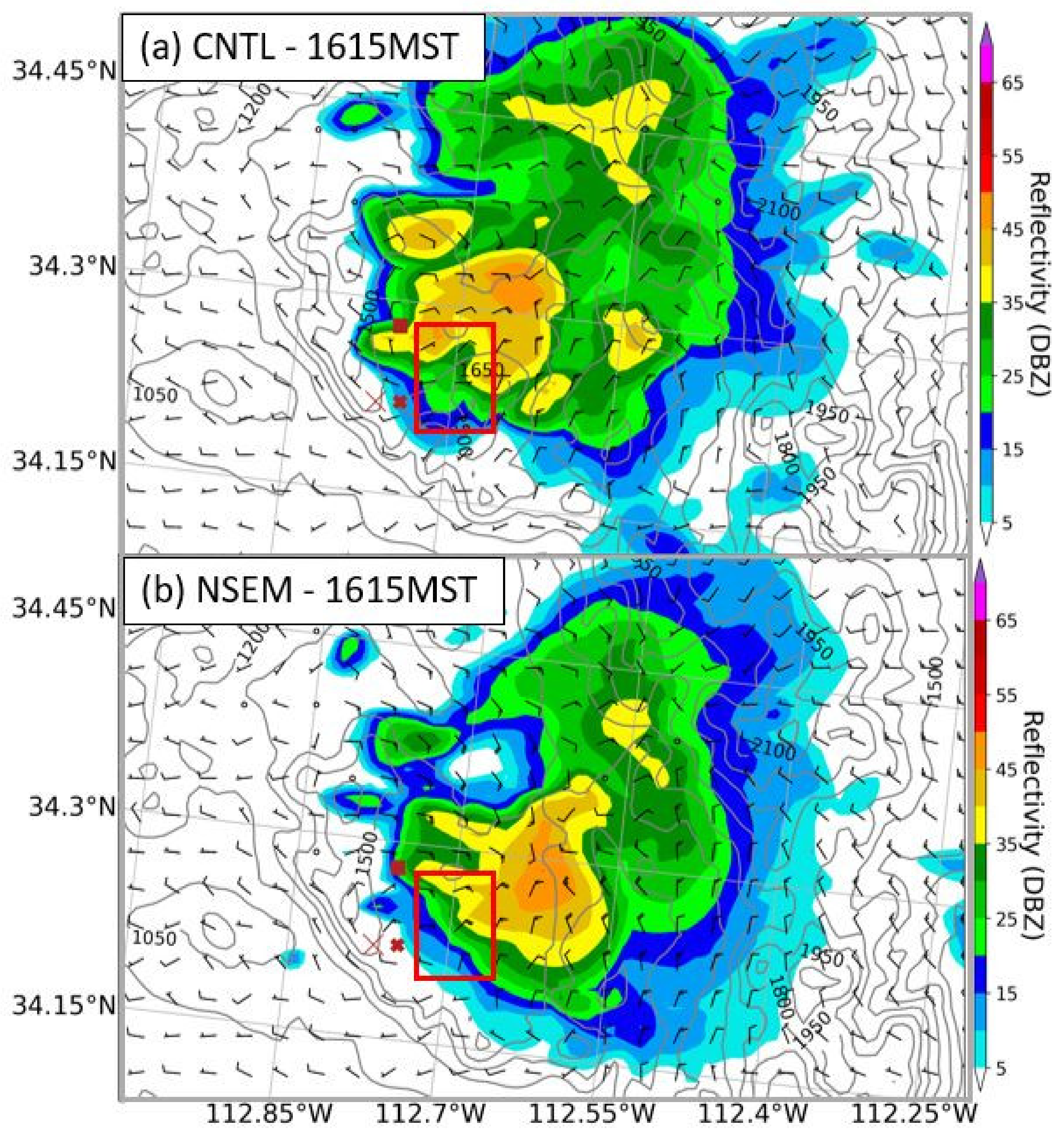
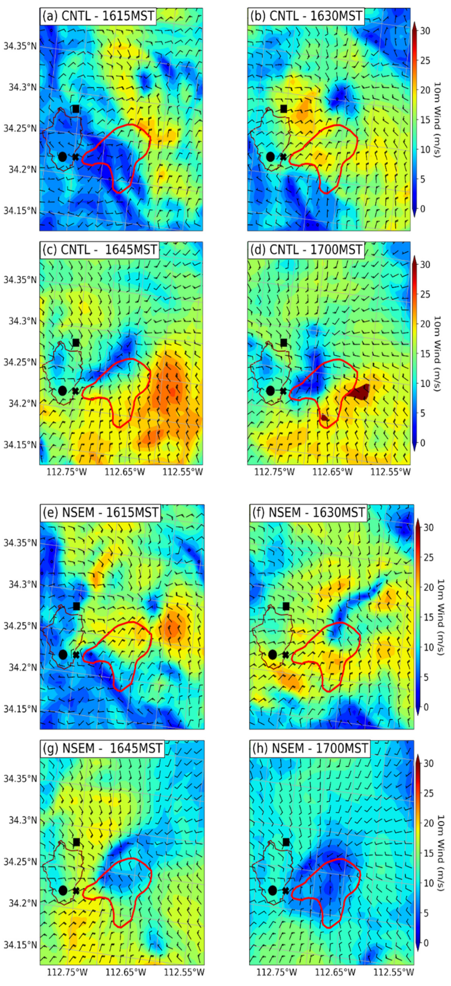
Examining the simulated reflectivity and 10 m winds (
Figure 14a), an outflow is shown that developed from convection just northeast of Yarnell (bold x) by 1615 MST. This convective cell generates two surges of momentum that divert to the south and west as the outflow encounters the isolated Weaver Mountain to the east of Yarnell. The southward-directed surge rushed into the eastern valley while the westward-directed surge rushed into the gap between the western and southeastern Weaver Mountains with velocities of 10–20 ms
−1 at 10 m above the ground. Examining the NSEM simulated reflectivity and 10 m winds (
Figure 14b), the same outflow is shown developing to the east-northeast of Yarnell around the same time, 1615 MST. However, without the influence of the southeast isolated Weaver Mountain, the flow does not divert as in the CNTL case and, instead, a broader fanning of momentum occurs which is stronger (15–20 ms
−1) but smoother (shown by the red square for the CNTL case and the NSEM case in
Figure 14) that rushes west, southwest, and south, toward and through the Granite Mountain Hotshots’ location just west of Yarnell (indicated by the thin x immediately west of Yarnell).
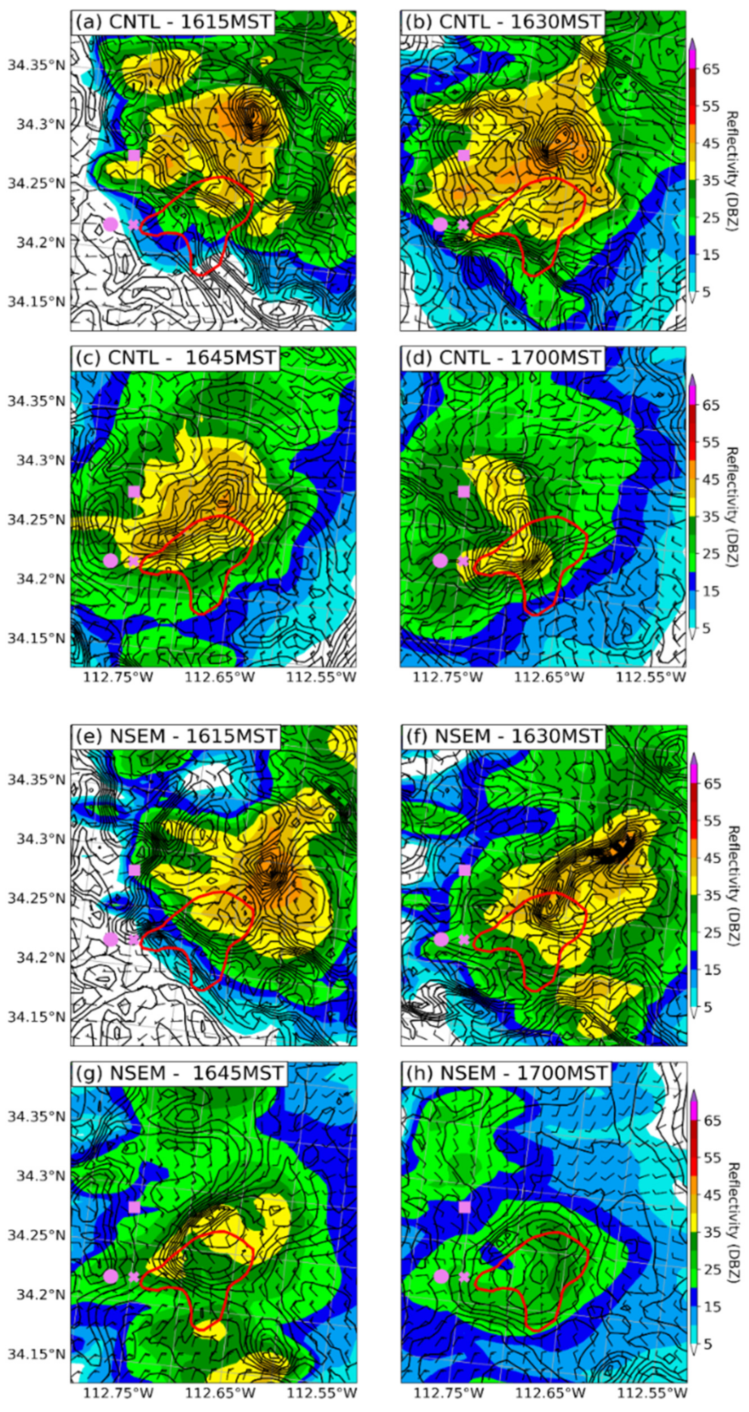
Figure 15 and
Figure 16 show the reflectivity and 10 m winds as contours, wind barbs, and shaded depictions and break down the outflow for the CNTL (a–d) and NSEM (e–h) cases from 1615 to 1700 MST. In the CNTL case, the outflow was generated near 34.33° N, 112.64° W. At 1615 MST, the eastern portion of the outflow is deflected into the eastern valley while it is being strengthened by the density current rushing through from the northeast (NEDC). By 1615–1630 MST, the head of the NEDC (first surge) rushes through the Hotshots’ location (circle), while right behind, to the northeast near Peeples Valley (square), the western part of the outflow (at 34.33° N, 112.64° W) also strengthens and merges with the remains of the NEDC from the northeast. The small portion of the outflow that makes it over the isolated Weaver Mountain, moves southwest over the terrain, and weakens. By 1630–1645 MST, the second surge (NEDC remains combined with the western portion of the outflow) moves through and past the Hotshots’ location with a more easterly component, as compared to the first surge of just the NEDC, which had a more northeasterly component.
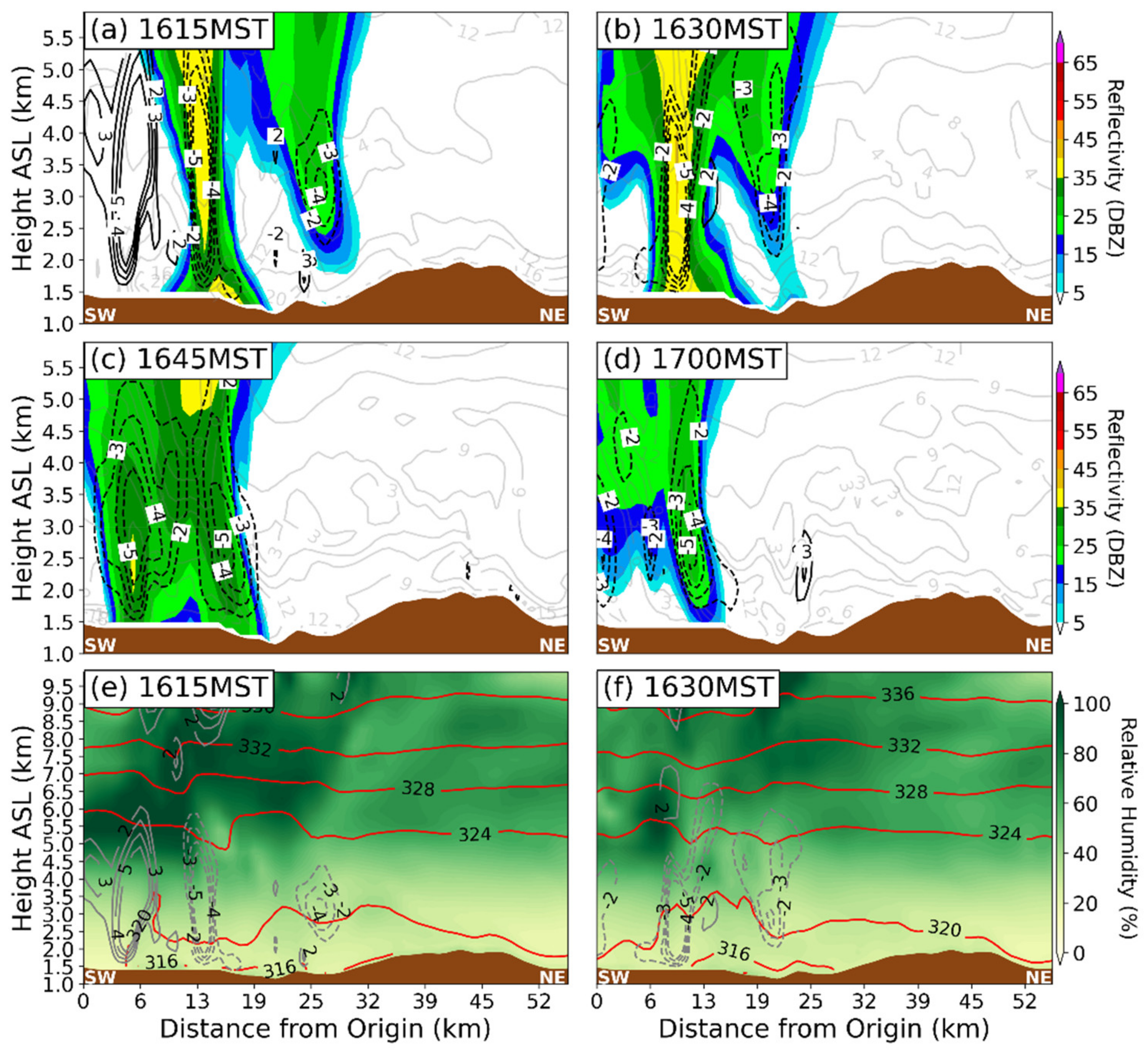
The cross-section used for the next CNTL and NSEM comparisons extending from Yarnell to just past the Bradshaw Mountains is denoted in
Figure 3a. In the CNTL case (
Figure 17), there is a speed reduction from 1630 to 1645 MST where the energy of the NEDC splits west and south as it encounters the isolated Weaver Mountain and merges with the outflow. The energy is more concentrated vertically than horizontally. The NSEM case (
Figure 18) shows the outflow with the density current from the northeast with little to no reduction in speed as it passes over the location of the southeast isolated Weaver Mountain. Despite more precipitation in the CNTL case, the density current is simulated to be stronger in the NSEM case, which also explains the stronger surges of the NEDC and the outflow near Peeples Valley.
The southeast isolated Weaver Mountain acts to weaken the momentum surges that move through the Hotshots’ locations. The first surge, the NEDC, splits and moves through that location from the northeast while an outflow is simultaneously generated further northeast which then merges with the remains of the NEDC and rushes through about 15 min later, with a more easterly component (second surge). The hypothesized splitting pattern was the motivation behind running the NSEM simulation to see the impact of the southeast isolated Weaver Mountain on the density current strength and propagation. From the reflectivity and winds (from
Figure 15 and
Figure 16), the origins of the second surge have a resemblance to a traveling microburst signature. This leads to suggest that the surge origins were not two density currents but rather a density current and a microburst outflow.
In the NSEM case, the outflow is generated in a similar location but more south (close to (34.3° N, 112.65° W)). Likewise, the outflow strengthens with the NEDC on the eastern side of the isolated Mountain by 1615 MST. From 1615 to 1630 MST, the head of the NEDC (first surge) rushes through the Hotshots’ location but slightly earlier than in the CNTL case. There is slightly less strengthening of the outflow on the western side near Peeples Valley as it merges with the remains of the NEDC, but the combination of flows ultimately becomes stronger than in the CNTL case. The portion of the outflow that moves to where the isolated Weaver Mountain would be exhibits less weakening and is maintained longer as it moves southwestward. From 1630 to 1645 MST, the second surge (again, remains of NEDC combined with the western portion of the outflow) moves through and past the Hotshots’ location with a more easterly (but stronger) component as well.
3.5. Interaction of Density Currents and Its Impacts on the Yarnell Hill Fire
This density current that affected the Yarnell Hill Fire on 30 June 2013 originated from convective storms toward the northeast over the Black Hills and propagated southwestwards. By the time the density current reached Peeples Valley, a smaller outflow originating from a small cell near Peeples Valley merged with the density current from the northeast. The resultant density current strengthened and propagated toward and over Yarnell and the fire environment (about 1645 MST in the observations and about 1615 MST in the case of the CNTL). The isolated southeast Weaver Mountain acts to deflect the density current into two components which move south and west. Without this deflection, the density current that shifted the Yarnell Hill Fire, first southeast then south, and then southwest, would have been much stronger in total momentum but perhaps not stronger exclusively in its westerly component and anticyclonic rotational structure. Two other major factors help to generate the density current, evaporative cooling and diurnal heating. The evaporative cooling helps to form the density current while diurnal heating helps to generate wind and pressure differences for the convection that spawned the density current. The presence of the isolated southeast Weaver Mountain (NSEM) helps to dampen the density current. The next section will cover HDW effects.
3.6. HDW Effects on the Yarnell Hill Fire
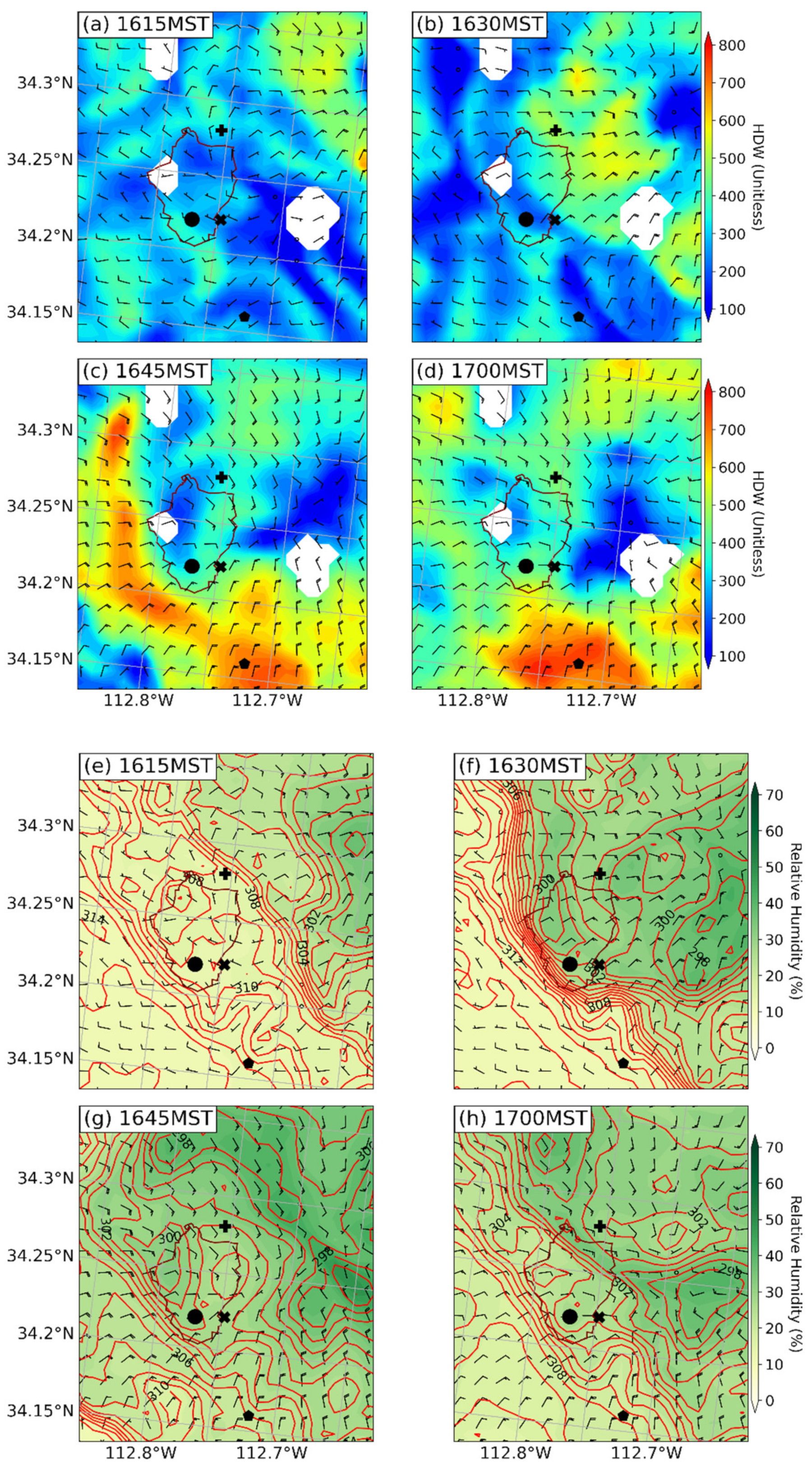
Figure 19 shows the calculated HDW (shaded contours) during the time of the fire incident as well as the 2 m relative humidity and temperature (red contours) and the 10 m horizontal wind (barbs), i.e., components of HDW, for the CNTL case from 1615 to 1700 MST. In the CNTL case, at the beginning of the time frame (at 1615 MST), HDW (a–d) over the fire environment is relatively low at about 200–350, with higher values toward the south. When the density current passes the region of interest, HDW rises to 400–500 starting at the northeastern portion of the fire by 1630 MST and moving south-southeast over the incident site. The entire fire environment is affected by larger HDW values except for the western portion, where the western Weaver Mountains are located since the maximum value there only reaches about 300. Surprisingly, the highest HDW values in the viewing region are not at the fire but rather toward the south and southwest, in the valley.
Breaking down HDW into its individual components reveals that not all the components need to drastically increase for HDW to be high. For example, in the case of the CNTL, from 1630 to 1645 MST, at the incident site the 2 m temperature slightly decreases by ~0.1 K while the dryness increases by about 5%, which lead to an increase in HDW. The most significant factor is the wind factor which creates the largest HDW increase from 1645 to 1700 MST.
HDW can also be compared to the observations. From
Table 4, the peak HDW, during the event, at Peeples Valley, occurs around 1725 MST with a value of 265, shortly after the last time frame in the simulations conducted in this study. The higher values from 1509 to 1539 MST can be explained by a quick wind shift, not from a density current, from WSW to SW that briefly advected hotter temperatures and reduced the moisture content which increased HDW for a short time (less than a 20-min period) which was not sustained long enough for significant fire effects. In
Table 5, at Stanton, the peak HDW occurs by 1701 MST reaching a value of about 570. Comparatively, the calculated HDW based on observations is lower by approximately 230 for Peeples Valley and for Stanton based on the maximum value obtained in the CNTL case. This difference can be explained by the larger simulated wind (7 ms
−1 observed, ~12 ms
−1 simulated) for Peeples Valley as well as Stanton (11 ms
−1 observed, ~12/s simulated). The simulation may represent the observed wind speed worse; however, this still indicates that the wind component seems to be the most sensitive to a change in HDW. For both locations, HDW rises from 1615 to 1700 MST in both the observations and in the CNTL simulation.
In reviewing the simulated wind speed and comparing it to observations, the CNTL simulation performed reasonably well in terms of wind direction and timing. However, for the wind magnitudes, an overall high bias was seen which was associated with weaker observed winds. The simulated winds in the CNTL case were higher than in the observations showing about 10–15 ms
−1 near Cherry, AZ, USA, in the simulation (near the surface on the right of
Figure 11e) but only about 5 ms
−1 in the observations (
Table 3). For Peeples Valley, the simulated wind magnitude showed about 12 ms
−1 (
Figure 16d) which was also higher than in the observations (
Table 3) which indicate only about 8 ms
−1. For Stanton, the simulated wind showed about 12 ms
−1 in both the CNTL simulation (
Figure 17d) and the observations (
Table 3). The timing and wind direction agreed between the CNTL simulation (
Figure 17) and the surface observations (
Table 3). The findings for the wind magnitude are similar to those found in the Dude Fire [
5] which had winds of 20 mph (9 m/s) for about 30 min. The high bias may arise out of too coarse of a grid spacing within the WRF model, since the WRF model has higher uncertainty depending on how the model is configured [
53]. This high bias could be resolved with an increased resolution. Although the highest resolution of this study (i.e., 0.777 km) may still not be fine enough to fully resolve the wind magnitudes, it does provide enough detail to resolve the density current and MPS signatures, two main factors of this study.
In reviewing the simulated relative humidity and comparing to observations, the results are in alignment. The simulated relative humidity (near the surface on the right of
Figure 13e) is near 20% at the approximate location of Cherry which agrees with the observations from the mid to late afternoon (
Table 3). For Peeples Valley, the simulated relative humidity (
Figure 19h) shows values near 25% which also agrees with the observations (
Table 3). For Stanton, the simulated relative humidity (
Figure 19h) shows low relative humidity values of 10–20%, which, once again are in agreement with the observations (
Table 3).
4. Conclusions and Discussions
This study has investigated factors that contributed to the generation of the density current and its wind shifts that suddenly redirected the Yarnell Hill Fire near Yarnell, Arizona, during the late afternoon of 30 June 2013. Four sensitivity tests were conducted using the Weather Research and Forecasting model with a minimum grid spacing of 0.777 km (D03). The four cases conducted were a control case (CNTL) for comparison, a case with the southeast isolated Weaver Mountain removed (NSEM) to study blocking effects, a case with evaporative cooling turned off (NEVP) to study the density current generation, and a case with the diurnal heating turned off (NDHT) to investigate the importance of daytime thermals to the generation of convection that leads to the density current.
The results have shown the remarkable similarity in convective initiation between the CNTL case and the observed radar reflectivity, where it was most vital. Nonetheless, the CNTL case still appears to be northwest biased overall in convective triggering with little to no convection toward the southeast. Fortunately, this has not significantly affected the analysis since the area of interest was relevant to the central part of the squall line that developed over central Yavapai County, AZ, USA. In the NEVP case, convection is also similarly initialized but the intensity remains weak, and the system remains stationary at the initiation location, resulting in an overall mismatch to the observed radar reflectivity. In the NDHT case, essentially no convection is generated since there is no surface sensible heating. Unsurprisingly, this case matches the least with the observed radar reflectivity.
The density current that was generated from the convection does not appear in the NEVP and NDHT cases. The convection that triggered the density current was strongly influenced by the MPS over the Black Hills which lifted moist air into the environment that spawned the thunderstorm complex and explains the origin of the convective initiation, at least for the CNTL case and the NEVP case. The MPS signature relies on surface sensible heating and the density current relies on evaporative cooling to be present. Thus, when turning off the evaporative cooling, the MPS is still present, but any convection remains constrained far above the surface since the lower levels cannot be cooled and moistened for precipitation to reach the surface. When turning off the surface sensible heating (diurnal heating), the MPS disappears. Thus, no convection is initialized over the Black Hills which means that no evaporative cooling was present to spawn the density current.
The Yarnell Hill Fire was affected by a sudden wind shift that rapidly redirected the fire front from moving east to south and then southwest which trapped and killed 19 firefighters. The wind shift originated from at least one density current by a thunderstorm complex that formed over the Black Hills. The wind shift origin and strength were affected by terrain and atmospheric processes. Overall, the results indicate that the effects of the evaporative cooling, which induced the pressure perturbation that generated the density current, played the most significant role in the density current generation. The effects of diurnal heating played the second-most significant role in the generation of the density current. Removing the diurnal heating removed the thunderstorm and, in extension, the density current, showing that the density current was not smoke induced nor from a front nor dryline. The effects of the southeast isolated Weaver Mountain played a role in reducing the strong mesoscale momentum and weakening the fire wind shift.
When the results were compared to the observations at Cherry, Peeples Valley, and Stanton, AZ, USA, the simulated wind magnitudes were higher than in the surface observations. The wind direction and timing, however, aligned well. The simulated and observed relative humidity at the three locations also aligned with the surface observations.
In addition to the sensitivity tests discussed, we also examined the role of HDW as a predictive tool for the fire. HDW was only explored for the CNTL case since cases NEVP and NDHT did not produce realistic wind shifts. The results have shown that HDW does predict the change in the fire environment since HDW values increase with the passing of the density current; however, a further study is needed to explore more fire-specific aspects using the WRF-Fire variant as part of the WRF model.
It is our goal in this manuscript to focus solely on the role of the environmental physical processes in causing the convectively induced rapid wind shifts that changed the environmental forcing surrounding the Yarnell Hill Fire. While we are not, in this manuscript, concerned about the feedback from explicit fire heating and related physical processes caused directly by the fire on the larger surrounding environment, the WRF-Fire version of the model would also help us understand the interaction of fire fuel and the atmospheric environment, if it is represented or parameterized in the model. We are focusing on the downscale environmental forcing of the fire and solely that. Additionally, the physical processes we are focusing on, while not every planetary boundary layer process, are what we consider to be the most significant elements in the low-level physical environment. Along this line of downscale modeling with a horizontal resolution of 0.777 km, it is important to mention that a further decrease in horizontal resolution will require large-eddy simulations (LES). Here, the vertical fluxes of moisture and momentum are no longer dominative; thus, the grid resolutions in the horizontal should be comparable to that in the vertical. Additionally, the PBL parameterizations in the WRF model would be less representative of the actual PBL processes.


