
Machine Learning to Predict Area Fugitive Emission Fluxes of GHGs from Open-Pit Mines


Abstract
:1. Introduction
1.1. Measurement Techniques to Quantify Emission Fluxes
1.2. Modeling Techniques to Quantify Emission Fluxes
1.3. Research Gaps and Objectives
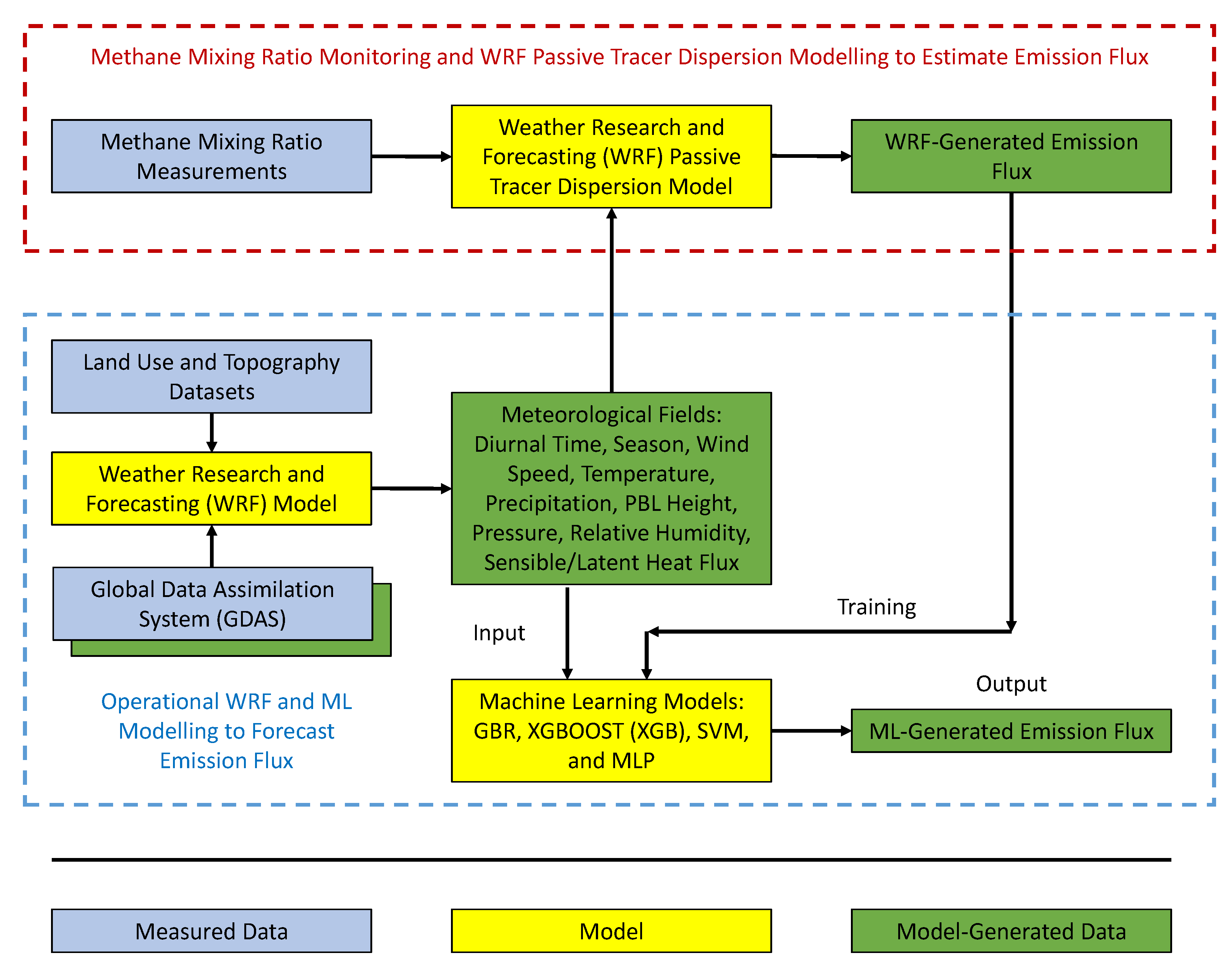
2. Methodology
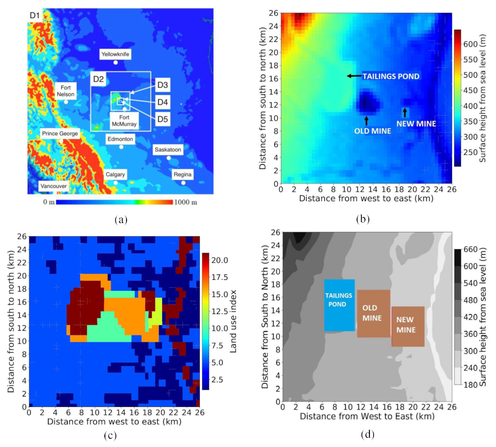
2.1. Open-Pit Mining Site
2.2. Weather Research and Forecasting Model
2.2.1. Model Configurations
2.2.2. Methane Transport and Flux Calculation
2.2.3. Uncertainty in WRF Estimate of the Methane Emission Flux
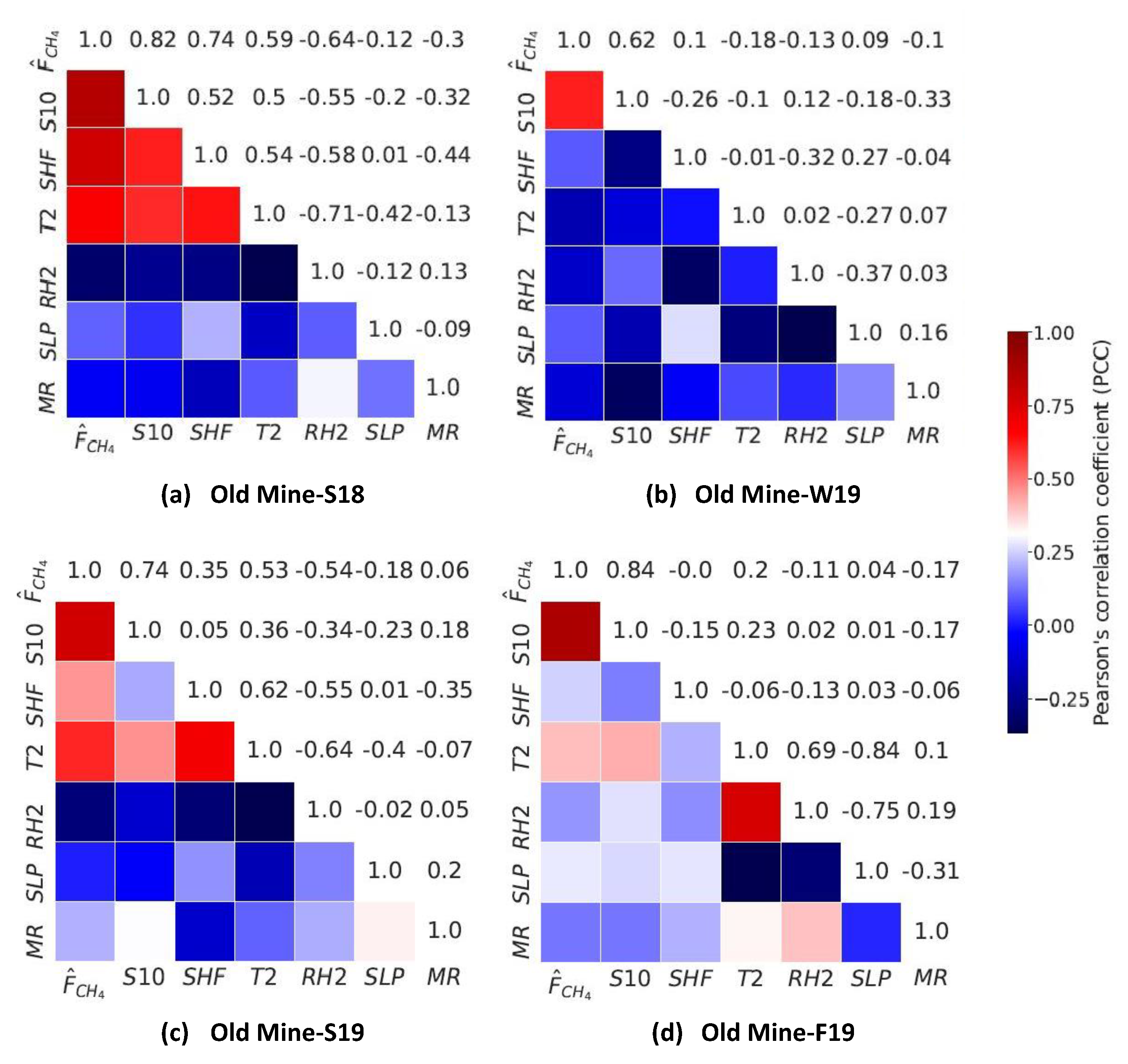
2.3. Machine Learning Model and Statistical Analysis
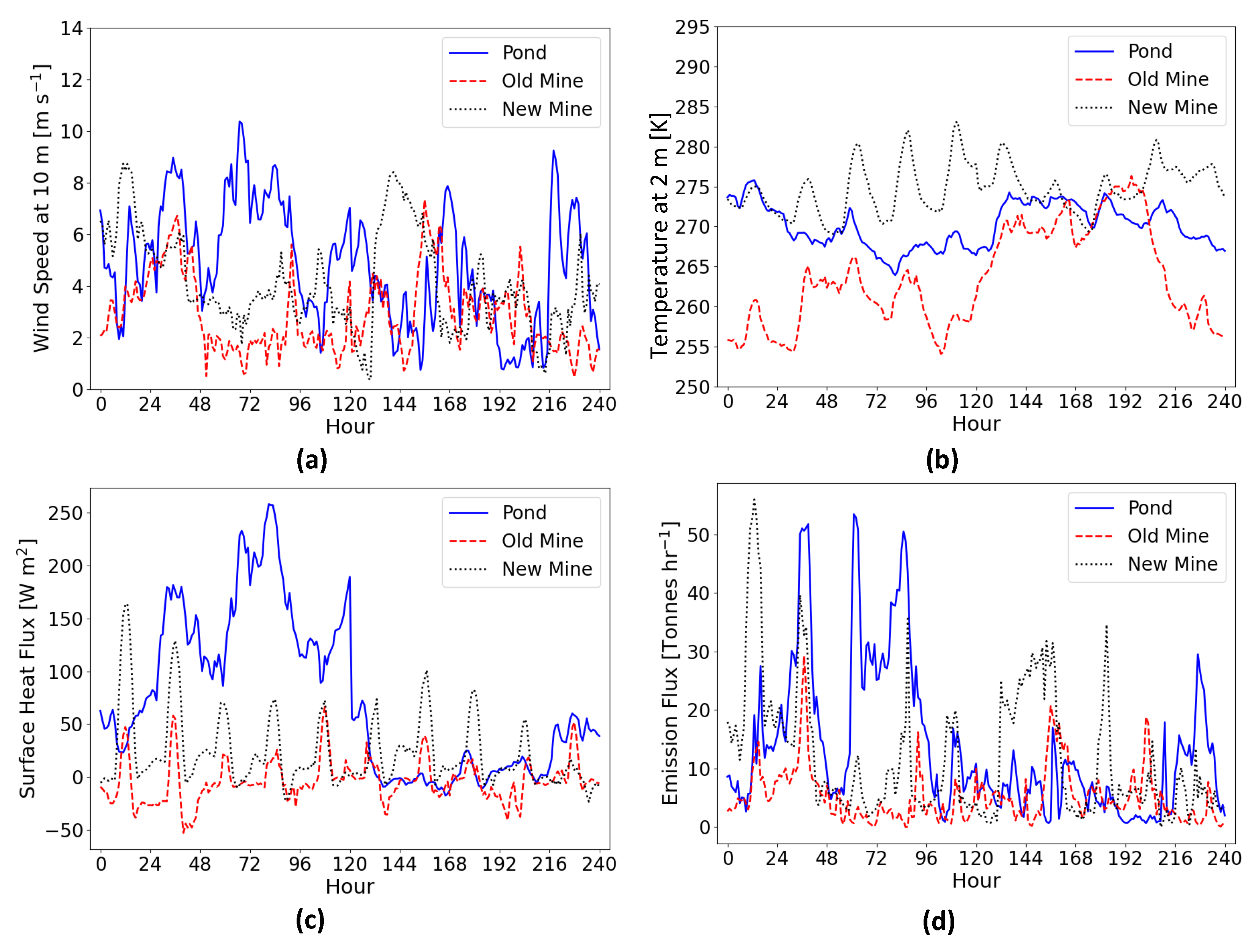
3. Results and Discussion
4. Conclusions and Recommendations
Author Contributions
Funding
Institutional Review Board Statement
Informed Consent Statement
Data Availability Statement
Acknowledgments
Conflicts of Interest
Nomenclature
| ΔA: | Area element (m2) |
| Bias: | Bias of emission flux (Tonne h−1) |
| F: | Emission flux (Tonne h−1) |
| M: | Modeled emission flux (Tonne h−1) |
| MR: | Methane mixing ratio (ppm) |
| n: | Sample size (-) |
| O: | Reference emission flux (Tonne h−1) |
| PCC: | Pearson’s correlation coefficient (-) |
| R2: | Coefficient of determination (-) |
| RH2: | Relative humidity at 2 m (%) |
| RMSE: | Root mean square error of emission flux (Tonne h−1) |
| : | Concentration of passive tracer (μg m−3) |
| SHF: | Surface Heat Flux (W m−2) |
| S10: | Wind speed at 10 m (m s−1) |
| SLP: | Sea level pressure (Pa) |
| T2: | Temperature at 2 m (K) |
| : | Average wind velocity along x direction (m s−1) |
| : | Average wind velocity along y direction (m s−1) |
| : | Average wind velocity along z direction (m s−1) |
Abbreviations
| ABL: | Atmospheric Boundary Layer |
| CALPUFF: | CALifornia PUFF Model |
| FCs: | Flux Chambers |
| GTOPO 30s: | Global 30 Arc-Second |
| GDAS: | Global Data Assimilation System |
| GBR: | Gradient Boosting |
| GHG: | Greenhouse Gas |
| IDM: | Inverse Dispersion Modelling |
| LS: | Land Surface |
| LSTM: | Long Short-Term Memory |
| LGR: | Los Gatos Research |
| ML: | Machine Learning |
| MODIS: | Moderate Resolution Imaging Spectroradiometer |
| MLP: | Multi-Layer Perceptron |
| NCEP: | National Centers for Environmental Prediction |
| PBL: | Planetary Boundary Layer |
| SRTM: | Shuttle Radar Topography Mission |
| SVM: | Support Vector Machines |
| SL: | Surface Layer |
| TKE: | Turbulence Kinetic Energy |
| WRF: | Weather Research and Forecasting |
| XGB: | XGBOOST |
References
- Betancourt-Torcat, A.; Elkamel, A.; Ricardez-Sandoval, L. A modeling study of the effect of carbon dioxide mitigation strategies, natural gas prices and steam consumption on the Canadian Oil Sands operations. Energy 2012, 45, 1018–1033. [Google Scholar] [CrossRef]
- Rahman, M.M.; Canter, C.; Kumar, A. Greenhouse gas emissions from recovery of various North American conventional crudes. Energy 2014, 74, 607–617. [Google Scholar] [CrossRef]
- Lan, X.; Talbot, R.; Laine, P.; Torres, A. Characterizing Fugitive Methane Emissions in the Barnett Shale Area Using a Mobile Laboratory. Environ. Sci. Technol. 2015, 49, 8139–8146. [Google Scholar] [CrossRef] [PubMed]
- Hendrick, M.F.; Ackley, R.; Sanaie-Movahed, B.; Tang, X.; Phillips, N.G. Fugitive methane emissions from leak-prone natural gas distribution infrastructure in urban environments. Environ. Pollut. 2016, 213, 710–716. [Google Scholar] [CrossRef] [PubMed] [Green Version]
- Ocko, I.B.; Hamburg, S.P.; Jacob, D.J.; Keith, D.W.; Keohane, N.O.; Oppenheimer, M.; Roy-Mayhew, J.D.; Schrag, D.P.; Pacala, S.W. Unmask temporal trade-offs in climate policy debates. Science 2017, 356, 492–493. [Google Scholar] [CrossRef]
- Höglund-Isaksson, L. Global anthropogenic methane emissions 2005-2030: Technical mitigation potentials and costs. Atmos. Chem. Phys. 2012, 12, 9079–9096. [Google Scholar] [CrossRef] [Green Version]
- Shindell, D.; Kuylenstierna, J.C.I.; Vignati, E.; van Dingenen, R.; Amann, M.; Klimont, Z.; Anenberg, S.C.; Muller, N.; Janssens-Maenhout, G.; Raes, F.; et al. Simultaneously Mitigating Near-Term Climate Change and Improving Human Health and Food Security. Science 2012, 335, 183–189. [Google Scholar] [CrossRef] [Green Version]
- Zhang, Y.; Gautam, R.; Pandey, S.; Omara, M.; Maasakkers, J.D.; Sadavarte, P.; Lyon, D.; Nesser, H.; Sulprizio, M.P.; Varon, D.J.; et al. Quantifying methane emissions from the largest oil-producing basin in the United States from space. Sci. Adv. 2020, 6. [Google Scholar] [CrossRef] [Green Version]
- Janzen, R.; Davis, M.; Kumar, A. Evaluating long-term greenhouse gas mitigation opportunities through carbon capture, utilization, and storage in the oil sands. Energy 2020, 209, 118364. [Google Scholar] [CrossRef]
- Nimana, B.; Canter, C.; Kumar, A. Life cycle assessment of greenhouse gas emissions from Canada’s oil sands-derived transportation fuels. Energy 2015, 88, 544–554. [Google Scholar] [CrossRef]
- Di Lullo, G.; Zhang, H.; Kumar, A. Uncertainty in well-to-tank with combustion greenhouse gas emissions of transportation fuels derived from North American crudes. Energy 2017, 128, 475–486. [Google Scholar] [CrossRef]
- Hmiel, B.; Petrenko, V.V.; Dyonisius, M.N.; Buizert, C.; Smith, A.M.; Place, P.F.; Harth, C.; Beaudette, R.; Hua, Q.; Yang, B.; et al. Preindustrial 14CH4 indicates greater anthropogenic fossil CH4 emissions. Nature 2020, 578, 409–412. [Google Scholar] [CrossRef] [PubMed]
- Hempel, S.; Adolphs, J.; Landwehr, N.; Willink, D.; Janke, D.; Amon, T. Supervised Machine Learning to Assess Methane Emissions of a Dairy Building with Natural Ventilation. Appl. Sci. 2020, 10, 6938. [Google Scholar] [CrossRef]
- Alvarez, R.A.; Zavala-Araiza, D.; Lyon, D.R.; Allen, D.T.; Barkley, Z.R.; Brandt, A.R.; Davis, K.J.; Herndon, S.C.; Jacob, D.J.; Karion, A.; et al. Assessment of methane emissions from the U.S. oil and gas supply chain. Science 2018, 361, 186–188. [Google Scholar] [CrossRef] [PubMed]
- Rotach, M.W.; Zardi, D. On the boundary-layer structure over highly complex terrain: Key findings from MAP. Q. J. R. Meteor. Soc. 2007, 133, 937–948. [Google Scholar] [CrossRef]
- Medeiros, L.E.; Fitzjarrald, D.R. Stable boundary layer in complex Terrain. Part I: Linking fluxes and intermittency to an average stability index. J. Appl. Meteorol. Clim. 2014, 53, 2196–2215. [Google Scholar] [CrossRef]
- Medeiros, L.E.; Fitzjarrald, D.R. Stable boundary layer in complex terrain. Part II: Geometrical and sheltering effects on mixing. J. Appl. Meteorol. Clim. 2015, 54, 170–188. [Google Scholar] [CrossRef]
- Soiket, M.I.; Oni, A.; Kumar, A. The development of a process simulation model for energy consumption and greenhouse gas emissions of a vapor solvent-based oil sands extraction and recovery process. Energy 2019, 173, 799–808. [Google Scholar] [CrossRef]
- Byerlay, R.A.E.; Nambiar, M.K.; Nazem, A.; Nahian, M.R.; Biglarbegian, M.; Aliabadi, A.A. Measurement of land surface temperature from oblique angle airborne thermal camera observations. Int. J. Remote Sens. 2020, 41, 3119–3146. [Google Scholar] [CrossRef]
- Nahian, M.R.; Nazem, A.; Nambiar, M.K.; Byerlay, R.; Mahmud, S.; Seguin, A.M.; Robe, F.R.; Ravenhill, J.; Aliabadi, A.A. Complex meteorology over a complex mining facility: Assessment of topography, land use, and grid spacing modifications in WRF. J. Appl. Meteorol. Clim. 2020, 59, 769–789. [Google Scholar] [CrossRef]
- Nambiar, M.K.; Byerlay, R.A.E.; Nazem, A.; Nahian, M.R.; Moradi, M.; Aliabadi, A.A. A Tethered Air Blimp (TAB) for observing the microclimate over a complex terrain. Geosci. Instrum. Meth. 2020, 9, 193–211. [Google Scholar] [CrossRef]
- Nambiar, M.K.; Robe, F.R.; Seguin, A.M.; Endsin, M.; Aliabadi, A.A. Diurnal and Seasonal Variation of Area-Fugitive Methane Advective Flux from an Open-Pit Mining Facility in Northern Canada Using WRF. Atmosphere 2020, 11, 1227. [Google Scholar] [CrossRef]
- Kia, S.; Flesch, T.K.; Freeman, B.S.; Aliabadi, A.A. Atmospheric transport over open-pit mines: The effects of thermal stability and mine depth. J. Wind Eng. Ind. Aerod. 2021, 214, 104677. [Google Scholar] [CrossRef]
- Kelly, E.N.; Schindler, D.W.; Hodson, P.V.; Short, J.W.; Radmanovich, R.; Nielsen, C.C. Oil sands development contributes elements toxic at low concentrations to the Athabasca River and its tributaries. Proc. Natl. Acad. Sci. USA 2010, 107, 16178–16183. [Google Scholar] [CrossRef] [PubMed] [Green Version]
- Small, C.C.; Cho, S.; Hashisho, Z.; Ulrich, A.C. Emissions from oil sands tailings ponds: Review of tailings pond parameters and emission estimates. J. Petrol. Sci. Eng. 2015, 127, 490–501. [Google Scholar] [CrossRef]
- Simpson, I.J.; Blake, N.J.; Barletta, B.; Diskin, G.S.; Fuelberg, H.E.; Gorham, K.; Huey, L.G.; Meinardi, S.; Rowland, F.S.; Vay, S.A.; et al. Characterization of trace gases measured over Alberta oil sands mining operations: 76 speciated C2–C10 volatile organic compounds (VOCs), CO2, CH4, CO, NO, NO2, NOy, O3 and SO2. Atmos. Chem. Phys. 2010, 10, 11931–11954. [Google Scholar] [CrossRef] [Green Version]
- Clements, C.B.; Whiteman, C.D.; Horel, J.D. Cold-Air-Pool Structure and Evolution in a Mountain Basin: Peter Sinks, Utah. J. Appl. Meteorol. 2003, 42, 752–768. [Google Scholar] [CrossRef]
- Whiteman, C.D.; Haiden, T.; Pospichal, B.; Eisenbach, S.; Steinacker, R. Minimum Temperatures, Diurnal Temperature Ranges, and Temperature Inversions in Limestone Sinkholes of Different Sizes and Shapes. J. Appl. Meteorol. 2004, 43, 1224–1236. [Google Scholar] [CrossRef]
- Bhowmick, T.; Bandopadhyay, S.; Ghosh, T. Three-dimensional CFD modeling approach to approximate air pollution conditions in high-latitude open-pit mines. WIT Trans. Built. Environ. 2015, 168, 741–753. [Google Scholar] [CrossRef] [Green Version]
- Silvester, S.A.; Lowndes, I.S.; Hargreaves, D.M. A computational study of particulate emissions from an open pit quarry under neutral atmospheric conditions. Atmos. Environ. 2009, 43, 6415–6424. [Google Scholar] [CrossRef]
- Liggio, J.; Li, S.M.; Staebler, R.M.; Hayden, K.; Darlington, A.; Mittermeier, R.L.; O’Brien, J.; McLaren, R.; Wolde, M.; Worthy, D.; et al. Measured Canadian oil sands CO2 emissions are higher than estimates made using internationally recommended methods. Nat. Commun. 2019, 10, 1863. [Google Scholar] [CrossRef] [PubMed]
- Rochette, P.; Eriksen-Hamel, N.S. Chamber measurements of soil Nitrous Oxide flux: Are absolute values reliable? Soil Sci. Soc. Am. J. 2008, 72, 331–342. [Google Scholar] [CrossRef]
- Bai, M.; Suter, H.; Lam, S.K.; Flesch, T.K.; Chen, D. Comparison of slant open-path flux gradient and static closed chamber techniques to measure soil N2O emissions. Atmos. Meas. Tech. 2019, 12, 1095–1102. [Google Scholar] [CrossRef] [Green Version]
- Meyers, T.P.; Hall, M.E.; Lindberg, S.E.; Kim, K. Use of the modified Bowen-ratio technique to measure fluxes of trace gases. Atmos. Environ. 1996, 30, 3321–3329. [Google Scholar] [CrossRef]
- Foken, T.; Leuning, R.; Oncley, S.R.; Mauder, M.; Aubinet, M. Eddy Covariance. In Eddy Covariance; Aubinet, M., Vesala, T., Papale, D., Eds.; Springer: Dordrecht, The Netherlands, 2012. [Google Scholar] [CrossRef]
- You, Y.; Staebler, R.M.; Moussa, S.G.; Beck, J.; Mittermeier, R.L. Methane emissions from an oil sands tailings pond: A quantitative comparison of fluxes derived by different methods. Atmos. Meas. Tech. 2021, 14, 1879–1892. [Google Scholar] [CrossRef]
- Gordon, M.; Li, S.M.; Staebler, R.; Darlington, A.; Hayden, K.; O’Brien, J.; Wolde, M. Determining air pollutant emission rates based on mass balance using airborne measurement data over the Alberta oil sands operations. Atmos. Meas. Tech. 2015, 8, 3745–3765. [Google Scholar] [CrossRef] [Green Version]
- Conley, S.; Faloona, I.; Mehrotra, S.; Suard, M.; Lenschow, D.H.; Sweeney, C.; Herndon, S.; Schwietzke, S.; Pétron, G.; Pifer, J.; et al. Application of Gauss’s theorem to quantify localized surface emissions from airborne measurements of wind and trace gases. Atmos. Meas. Tech. 2017, 10, 3345–3358. [Google Scholar] [CrossRef] [Green Version]
- Baray, S.; Darlington, A.; Gordon, M.; Hayden, K.L.; Leithead, A.; Li, S.M.; Liu, P.S.K.; Mittermeier, R.L.; Moussa, S.G.; O’Brien, J.; et al. Quantification of methane sources in the Athabasca Oil Sands Region of Alberta by aircraft mass balance. Atmos. Chem. Phys. 2018, 18, 7361–7378. [Google Scholar] [CrossRef] [Green Version]
- Flesch, T.K.; Wilson, J.D.; Harper, L.A.; Crenna, B.P. Estimating gas emissions from a farm with an inverse-dispersion technique. Atmos. Environ. 2005, 39, 4863–4874. [Google Scholar] [CrossRef]
- Pernini, T.G.; Zaccheo, T.S.; Dobler, J.; Blume, N. Estimating oil sands emissions using horizontal path-integrated column measurements. Atmos. Meas. Tech. 2022, 15, 225–240. [Google Scholar] [CrossRef]
- Scire, J.S.; Strimaitis, D.G.; Yamartino, R.J. A User’s Guide for the CALPUFF Dispersion Model (Version 5); Technical Report; Earth Tech, Inc.: Concord, MA, USA, 2000. [Google Scholar]
- Jittra, N.; Pinthong, N.; Thepanondh, S. Performance evaluation of AERMOD and CALPUFF air dispersion models in industrial complex area. Air Soil Water Res. 2015, 8, ASWR–S32781. [Google Scholar] [CrossRef] [Green Version]
- Arregocés, H.; Rojano, R.; Restrepo, G.; Angulo, L. Using CALPUFF to determine the environmental impact of a coal mine open pit. WIT Trans. Ecol. Environ. 2016, 207, 55–66. [Google Scholar] [CrossRef] [Green Version]
- Holnicki, P.; Kałuszko, A.; Nahorski, Z.; Stankiewicz, K.; Trapp, W. Air quality modeling for Warsaw agglomeration. Arch. Environ. Prot. 2017, 43, 48–64. [Google Scholar] [CrossRef] [Green Version]
- Oleniacz, R.; Rzeszutek, M. Intercomparison of the CALMET/CALPUFF modeling system for selected horizontal grid resolutions at a local scale: A case study of the MSWI Plant in Krakow, Poland. Appl. Sci. 2018, 8, 2301. [Google Scholar] [CrossRef] [Green Version]
- Rzeszutek, M. Parameterization and evaluation of the CALMET/CALPUFF model system in near-field and complex terrain-Terrain data, grid resolution and terrain adjustment method. Sci. Total Environ. 2019, 689, 31–46. [Google Scholar] [CrossRef]
- Sówka, I.; Paciorek, M.; Skotak, K.; Kobus, D.; Zathey, M.; Klejnowski, K. The Analysis of the Effectiveness of Implementing Emission Reduction Measures in Improving Air Quality and Health of the Residents of a Selected Area of the Lower Silesian Voivodship. Energies 2020, 13, 4001. [Google Scholar] [CrossRef]
- Cox, R.M.; Sontowski, J.; Dougherty, C.M. An evaluation of three diagnostic wind models (CALMET, MCSCIPUF, and SWIFT) with wind data from the Dipole Pride 26 field experiments. Meteorol. Appl. 2005, 12, 329–341. [Google Scholar] [CrossRef]
- Cui, H.; Yao, R.; Chen, L.; Lv, M.; Xin, C.; Wu, Q. Field study of atmospheric boundary layer observation in a hilly Gobi Desert region and comparison with the CALMET/CALPUFF model. Atmos. Environ. 2020, 235, 117576. [Google Scholar] [CrossRef]
- Wang, W.; Shaw, W.J.; Seiple, T.E.; Rishel, J.P.; Xie, Y. An evaluation of a diagnostic wind model (CALMET). J. Appl. Meteorol. Clim. 2008, 47, 1739–1756. [Google Scholar] [CrossRef]
- Qiu, X.; Cheng, I.; Yang, F.; Horb, E.; Zhang, L.; Harner, T. Emissions databases for polycyclic aromatic compounds in the Canadian Athabasca oil sands region—Development using current knowledge and evaluation with passive sampling and air dispersion modelling data. Atmos. Chem. Phys. 2018, 18, 3457–3467. [Google Scholar] [CrossRef] [Green Version]
- Gilliam, R.C.; Pleim, J.E. Performance assessment of new land surface and planetary boundary layer physics in the WRF-ARW. J. Appl. Meteorol. Clim. 2010, 49, 760–774. [Google Scholar] [CrossRef]
- Nossent, J.; Elsen, P.; Bauwens, W. Sobol’ sensitivity analysis of a complex environmental model. Environ. Modell. Softw. 2011, 26, 1515–1525. [Google Scholar] [CrossRef]
- Jiménez, P.A.; Dudhia, J. Improving the representation of resolved and unresolved topographic effects on surface wind in the WRF model. J. Appl. Meteorol. Clim. 2012, 51, 300–316. [Google Scholar] [CrossRef] [Green Version]
- Lorente-Plazas, R.; Jiménez, P.A.; Dudhia, J.; Montávez, J.P. Evaluating and improving the impact of the atmospheric stability and orography on surface winds in the WRF model. Mon. Weather Rev. 2016, 144, 2685–2693. [Google Scholar] [CrossRef]
- Cerlini, P.B.; Emanuel, K.A.; Todini, E. Orographic effects on convective precipitation and space-time rainfall variability: Preliminary results. Hydrol. Earth Syst. Sci. 2005, 9, 285–299. [Google Scholar] [CrossRef]
- Rong, Z.; Dahai, X. Multi-scale turbulent planetary boundary layer parameterization in mesoscale numerical simulation. J. Appl. Meteorol. Sci. 2004, 15, 543–555. [Google Scholar]
- Houze, R.A., Jr. Orographic effects on precipitating clouds. Rev. Geophys. 2012, 50, RG1001. [Google Scholar] [CrossRef]
- Yáñez-Morroni, G.; Gironás, J.; Caneo, M.; Delgado, R.; Garreaud, R. Using the Weather Research and Forecasting (WRF) model for precipitation forecasting in an Andean region with complex topography. Atmosphere 2018, 9, 304. [Google Scholar] [CrossRef] [Green Version]
- Taylor, C.M.; Lambin, E.F.; Stephenne, N.; Harding, R.J.; Essery, R.L. The influence of land use change on climate in the Sahel. J. Clim. 2002, 15, 3615–3629. [Google Scholar] [CrossRef]
- De Meij, A.; Vinuesa, J. Impact of SRTM and Corine Land Cover data on meteorological parameters using WRF. Atmos. Res. 2014, 143, 351–370. [Google Scholar] [CrossRef]
- Zhang, C.; Lin, H.; Chen, M.; Yang, L. Scale matching of multiscale digital elevation model (DEM) data and the Weather Research and Forecasting (WRF) model: A case study of meteorological simulation in Hong Kong. Arab. J. Geosci. 2014, 7, 2215–2223. [Google Scholar] [CrossRef]
- Blaylock, B.K.; Horel, J.D.; Crosman, E.T. Impact of Lake Breezes on Summer Ozone Concentrations in the Salt Lake Valley. J. Appl. Meteorol. Climatol. 2017, 56, 353–370. [Google Scholar] [CrossRef]
- Bhimireddy, S.R.; Bhaganagar, K. Short-term passive tracer plume dispersion in convective boundary layer using a high-resolution WRF-ARW model. Atmos. Pollut. Res. 2018, 9, 901–911. [Google Scholar] [CrossRef]
- Grell, G.A.; Peckham, S.E.; Schmitz, R.; McKeen, S.A.; Frost, G.; Skamarock, W.C.; Eder, B. Fully coupled online chemistry within the WRF model. Atmos. Environ. 2005, 39, 6957–6975. [Google Scholar] [CrossRef]
- Beck, V.; Gerbig, C.; Koch, T.; Bela, M.M.; Longo, K.M.; Freitas, S.R.; Kaplan, J.O.; Prigent, C.; Bergamaschi, P.; Heimann, M. WRF-Chem simulations in the Amazon region during wet and dry season transitions: Evaluation of methane models and wetland inundation maps. Atmos. Chem. Phys. 2013, 13, 7961–7982. [Google Scholar] [CrossRef] [Green Version]
- Ahmadov, R.; McKeen, S.; Trainer, M.; Banta, R.; Brewer, A.; Brown, S.; Edwards, P.M.; de Gouw, J.A.; Frost, G.J.; Gilman, J.; et al. Understanding high wintertime ozone pollution events in an oil- and natural gas-producing region of the western US. Atmos. Chem. Phys. 2015, 15, 411–429. [Google Scholar] [CrossRef] [Green Version]
- Barkley, Z.R.; Lauvaux, T.; Davis, K.J.; Deng, A.; Miles, N.L.; Richardson, S.J.; Cao, Y.; Sweeney, C.; Karion, A.; Smith, M.; et al. Quantifying methane emissions from natural gas production in north-eastern Pennsylvania. Atmos. Chem. Phys. 2017, 17, 13941–13966. [Google Scholar] [CrossRef] [Green Version]
- Leukauf, D.; Gohm, A.; Rotach, M.W. Quantifying horizontal and vertical tracer mass fluxes in an idealized valley during daytime. Atmos. Chem. Phys. 2016, 16, 13049–13066. [Google Scholar] [CrossRef] [Green Version]
- Karion, A.; Lauvaux, T.; Lopez Coto, I.; Sweeney, C.; Mueller, K.; Gourdji, S.; Angevine, W.; Barkley, Z.; Deng, A.; Andrews, A.; et al. Intercomparison of atmospheric trace gas dispersion models: Barnett Shale case study. Atmos. Chem. Phys. 2019, 19, 2561–2576. [Google Scholar] [CrossRef] [Green Version]
- Zhao, X.; Marshall, J.; Hachinger, S.; Gerbig, C.; Frey, M.; Hase, F.; Chen, J. Analysis of total column CO2 and CH4 measurements in Berlin with WRF-GHG. Atmos. Chem. Phys. 2019, 19, 11279–11302. [Google Scholar] [CrossRef] [Green Version]
- Cortes, C.; Vapnik, V. Support-vector networks. Mach. Learn. 1995, 20, 273–297. [Google Scholar] [CrossRef]
- Maier, H.R.; Dandy, G.C. The use of artificial neural networks for the prediction of water quality parameters. Water Resour. Res. 1996, 32, 1013–1022. [Google Scholar] [CrossRef]
- Piryonesi, S.M.; El-Diraby, T.E. Data analytics in asset management: Cost-effective prediction of the pavement condition index. J. Infrastruct. Syst. 2020, 26, 04019036. [Google Scholar] [CrossRef]
- Hochreiter, S.; Schmidhuber, J. Long short-term memory. Neural Comput. 1997, 9, 1735–1780. [Google Scholar] [CrossRef] [PubMed]
- Freeman, B.S.; Taylor, G.; Gharabaghi, B.; Thé, J. Forecasting air quality time series using deep learning. J. Air Waste Manag. 2018, 68, 866–886. [Google Scholar] [CrossRef]
- Tabrizi, S.E.; Xiao, K.; Van Griensven, J.; Saad, M.; Farghaly, H.; Yang, S.X.; Gharabaghi, B. Hourly Road Pavement Surface Temperature Forecasting Using Deep Learning Modelsa. J. Hydrol. 2021, 603, 126877. [Google Scholar] [CrossRef]
- Skrobek, D.; Krzywanski, J.; Sosnowski, M.; Kulakowska, A.; Zylka, A.; Grabowska, K.; Ciesielska, K.; Nowak, W. Prediction of Sorption Processes Using the Deep Learning Methods (Long Short-Term Memory). Energies 2020, 13, 6601. [Google Scholar] [CrossRef]
- Ashraf, W.M.; Uddin, G.M.; Arafat, S.M.; Krzywanski, J.; Xiaonan, W. Strategic-level performance enhancement of a 660 MWe supercritical power plant and emissions reduction by AI approach. Energy Convers. Manag. 2021, 250, 114913. [Google Scholar] [CrossRef]
- Ashraf, W.M.; Uddin, G.M.; Farooq, M.; Riaz, F.; Ahmad, H.A.; Kamal, A.H.; Anwar, S.; El-Sherbeeny, A.M.; Khan, M.H.; Hafeez, N.; et al. Construction of Operational Data-Driven Power Curve of a Generator by Industry 4.0 Data Analytics. Energies 2021, 14, 1227. [Google Scholar] [CrossRef]
- Powers, J.G.; Klemp, J.B.; Skamarock, W.C.; Davis, C.A.; Dudhia, J.; Gill, D.O.; Coen, J.L.; Gochis, D.J.; Ahmadov, R.; Peckham, S.E.; et al. The weather research and forecasting model: Overview, system efforts, and future directions. B. Am. Meteorol. Soc. 2017, 98, 1717–1737. [Google Scholar] [CrossRef]
- Janjić, Z.I. The Step-Mountain Eta Coordinate Model: Further Developments of the Convection, Viscous Sublayer, and Turbulence Closure Schemes. Mon. Weather Rev. 1994, 122, 927–945. [Google Scholar] [CrossRef] [Green Version]
- Thompson, G.; Field, P.R.; Rasmussen, R.M.; Hall, W.D. Explicit Forecasts of Winter Precipitation Using an Improved Bulk Microphysics Scheme. Part II: Implementation of a New Snow Parameterization. Mon. Weather Rev. 2008, 136, 5095–5115. [Google Scholar] [CrossRef]
- Iacono, M.J.; Delamere, J.S.; Mlawer, E.J.; Shephard, M.W.; Clough, S.A.; Collins, W.D. Radiative forcing by long-lived greenhouse gases: Calculations with the AER radiative transfer models. J. Geophys. Res. Atmos. 2008, 113, D13103. [Google Scholar] [CrossRef]
- Zhang, C.; Wang, Y.; Hamilton, K. Improved Representation of Boundary Layer Clouds over the Southeast Pacific in ARW-WRF Using a Modified Tiedtke Cumulus Parameterization Scheme. Mon. Weather Rev. 2011, 139, 3489–3513. [Google Scholar] [CrossRef] [Green Version]
- Lupaşcu, A.; Iriza, A.; Dumitrache, R. Using a high resolution topographic data set and analysis of the impact on the forecast of meteorological parameters. Rom. Rep. Phys. 2015, 67, 653–664. [Google Scholar]
- Friedl, M.A.; Sulla-Menashe, D.; Tan, B.; Schneider, A.; Ramankutty, N.; Sibley, A.; Huanga, X. MODIS Collection 5 global land cover: Algorithm refinements and characterization of new datasets. Remote Sens. Environ. 2010, 114, 168–182. [Google Scholar] [CrossRef]
- Subin, Z.M.; Riley, W.J.; Mironov, D. An improved lake model for climate simulations: Model structure, evaluation, and sensitivity analyses in CESM1. J. Adv. Model. Earth Syst. 2012, 4, M02001. [Google Scholar] [CrossRef]
- Gu, H.; Jin, J.; Wu, Y.; Ek, M.B.; Subin, Z.M. Calibration and validation of lake surface temperature simulations with the coupled WRF-lake model. Clim. Chang. 2015, 129, 471–483. [Google Scholar] [CrossRef]
- Allen, G.; Hollingsworth, P.; Kabbabe, K.; Pitt, J.R.; Mead, M.I.; Illingworth, S.; Roberts, G.; Bourn, M.; Shallcross, D.E.; Percival, C.J. The development and trial of an unmanned aerial system for the measurement of methane flux from landfill and greenhouse gas emission hotspots. Waste Manag. 2019, 87, 883–892. [Google Scholar] [CrossRef]
- Gibbs, J.A.; Fedorovich, E.; van Eijk, A.M.J. Evaluating Weather Research and Forecasting (WRF) Model Predictions of Turbulent Flow Parameters in a Dry Convective Boundary Layer. J. Appl. Meteorol. Climatol. 2011, 50, 2429–2444. [Google Scholar] [CrossRef]
- Xue, L.; Chu, X.; Rasmussen, R.; Breed, D.; Boe, B.; Geerts, B. The Dispersion of Silver Iodide Particles from Ground-Based Generators over Complex Terrain. Part II: WRF Large-Eddy Simulations versus Observations. J. Appl. Meteorol. Climatol. 2014, 53, 1342–1361. [Google Scholar] [CrossRef] [Green Version]
- Oertel, C.; Matschullat, J.; Zurba, K.; Zimmermann, F.; Erasmi, S. Greenhouse gas emissions from soils—A review. Geochemistry 2016, 76, 327–352. [Google Scholar] [CrossRef] [Green Version]
- Hunter, J.D. Matplotlib: A 2D graphics environment. Comput. Sci. Eng. 2007, 9, 90–95. [Google Scholar] [CrossRef]
- Waskom, M.L. seaborn: Statistical data visualization. J. Open Source Softw. 2021, 6, 3021. [Google Scholar] [CrossRef]
- Pedregosa, F.; Varoquaux, G.; Gramfort, A.; Michel, V.; Thirion, B.; Grisel, O.; Blondel, M.; Prettenhofer, P.; Weiss, R.; Dubourg, V.; et al. Scikit-learn: Machine Learning in Python. J. Mach. Learn. Res. 2011, 12, 2825–2830. [Google Scholar]
- Buitinck, L.; Louppe, G.; Blondel, M.; Pedregosa, F.; Mueller, A.; Grisel, O.; Niculae, V.; Prettenhofer, P.; Gramfort, A.; Grobler, J.; et al. API design for machine learning software: Experiences from the scikit-learn project. In Proceedings of the European Conference on Machine Learning and Principles and Practice of Knowledge Discovery In Databases: Languages for Data Mining and Machine Learning, Prague, Czech Republic, 23–27 September 2013; pp. 108–122. [Google Scholar]
- Chen, T.; Guestrin, C. XGBoost: A Scalable Tree Boosting System. In Proceedings of the 22nd ACM SIGKDD International Conference on Knowledge Discovery and Data Mining, San Francisco, CA, USA, 13–17 August 2016; pp. 785–794. [Google Scholar] [CrossRef] [Green Version]


| Campaign | Year | Tailings Pond | Old Mine | New Mine |
|---|---|---|---|---|
| S18 | 2018 | 1 May–11 May | 18 May–28 May | - |
| W19 | 2019 | 14 February–24 February | 16 March–26 March | - |
| S19 | 2019 | 9 July–19 July | 29 July–8 August | 12 August–22 August |
| F19 | 2019 | 25 October–4 November | 10 November–20 November | 8 October–18 October |
| Physics | Parameterization |
|---|---|
| Planetary Boundary Layer (PBL) | Mellor-Yamada-Janić [83] |
| Microphysics | Thompson Parameterization [84] (D1, D2, and D3 only) |
| Longwave Radiation | Rapid Radiative Transfer Model [85] |
| Shortwave Radiation | Rapid Radiative Transfer Model [85] |
| Cumulus Parameterization | Tiedtke Parameterization [86] (D1, D2, and D3 only) |
| Surface Layer (SL) | Monin-Obukhov Eta Similarity Parameterization [83] |
| Land Surface (LS) | Noah Land Surface Parameterization |
| Old Mine (S18, W19, S19, F19) | New Mine (S19, F19) | Pond (S18, W19, S19, F19) | |||||
|---|---|---|---|---|---|---|---|
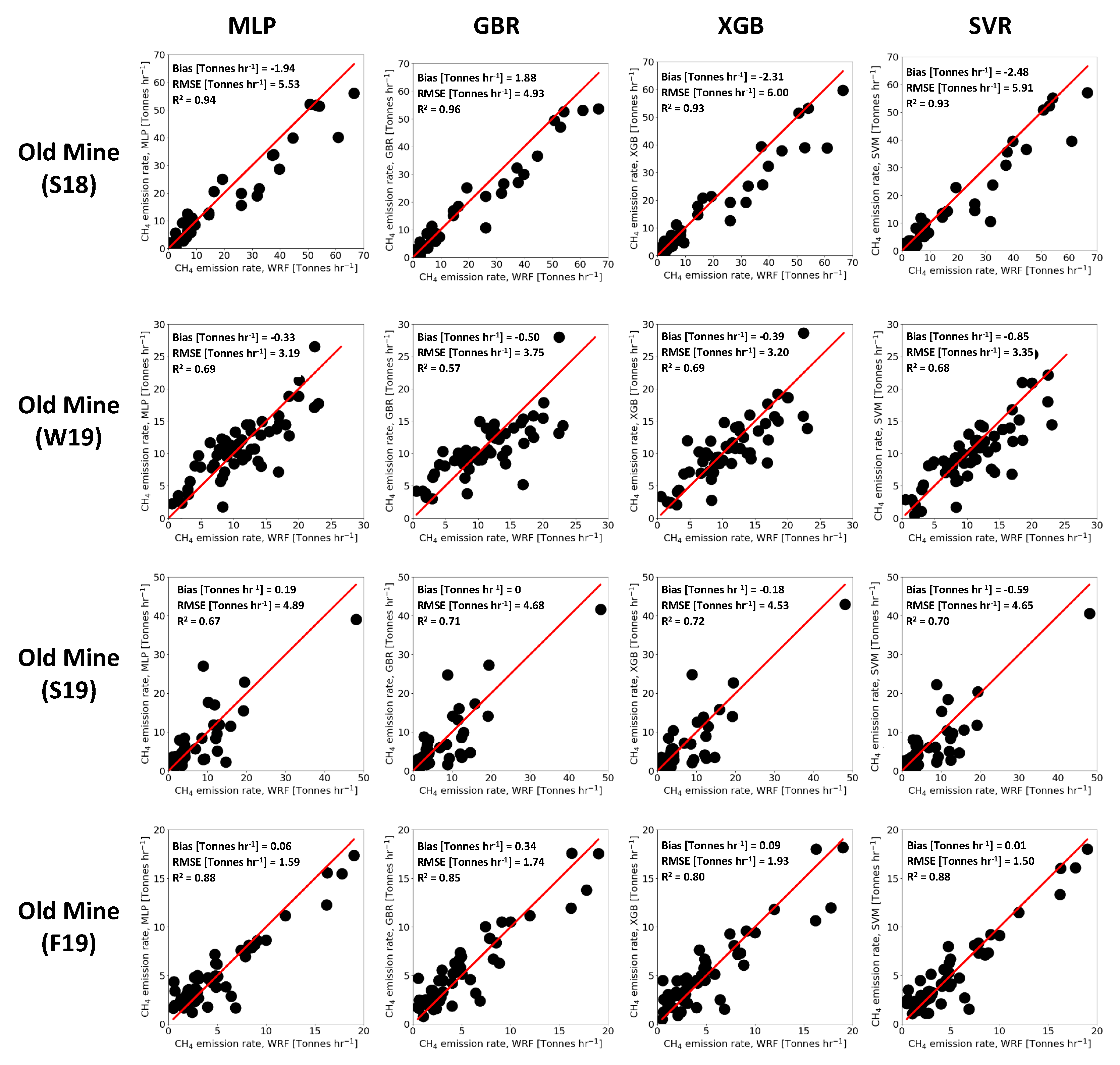
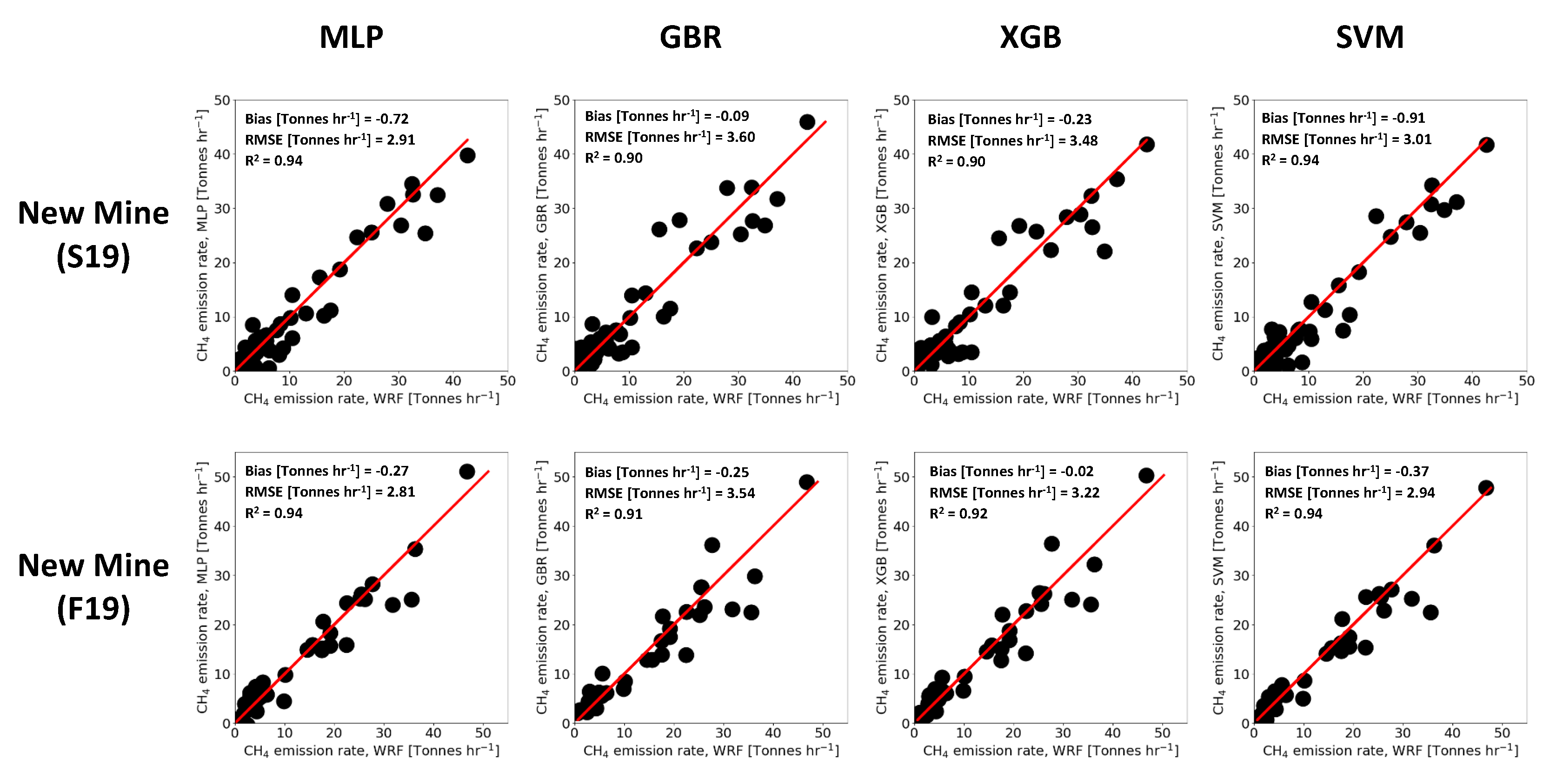
| Bias (Tonnes h) | MLP | −0.47 | Average = −0.62 | −0.51 | Average = −0.37 | 0.25 | Average = 0.03 |
| GBR | −0.46 | −0.17 | 0.11 | ||||
| XGB | −0.63 | −0.13 | −0.06 | ||||
| SVM | −0.91 | −0.65 | −0.20 | ||||
| RMSE (Tonnes h) | MLP | 3.93 | Average = 3.96 | 2.87 | Average = 3.20 | 3.75 | Average = 3.73 |
| GBR | 3.85 | 3.57 | 3.96 | ||||
| XGB | 4.04 | 3.36 | 3.81 | ||||
| SVM | 4.02 | 2.98 | 3.38 | ||||
| R (-) | MLP | 0.89 | Average = 0.89 | 0.94 | Average = 0.92 | 0.85 | Average = 0.85 |
| GBR | 0.89 | 0.90 | 0.83 | ||||
| XGB | 0.88 | 0.91 | 0.84 | ||||
| SVM | 0.89 | 0.94 | 0.88 | ||||
Publisher’s Note: MDPI stays neutral with regard to jurisdictional claims in published maps and institutional affiliations. |
© 2022 by the authors. Licensee MDPI, Basel, Switzerland. This article is an open access article distributed under the terms and conditions of the Creative Commons Attribution (CC BY) license (https://creativecommons.org/licenses/by/4.0/).
Share and Cite
Kia, S.; Nambiar, M.K.; Thé, J.; Gharabaghi, B.; Aliabadi, A.A. Machine Learning to Predict Area Fugitive Emission Fluxes of GHGs from Open-Pit Mines. Atmosphere 2022, 13, 210. https://doi.org/10.3390/atmos13020210
Kia S, Nambiar MK, Thé J, Gharabaghi B, Aliabadi AA. Machine Learning to Predict Area Fugitive Emission Fluxes of GHGs from Open-Pit Mines. Atmosphere. 2022; 13(2):210. https://doi.org/10.3390/atmos13020210
Chicago/Turabian StyleKia, Seyedahmad, Manoj K. Nambiar, Jesse Thé, Bahram Gharabaghi, and Amir A. Aliabadi. 2022. "Machine Learning to Predict Area Fugitive Emission Fluxes of GHGs from Open-Pit Mines" Atmosphere 13, no. 2: 210. https://doi.org/10.3390/atmos13020210