Severe Precipitation Phenomena in Crimea in Relation to Atmospheric Circulation

Abstract

The increase in the frequency and intensity of hazardous hydrometeorological phenomena is one of the most dangerous consequences of climate instability. In this study, we summarize the data on severe weather phenomena using the data from 23 meteorological stations in Crimea from 1976 to 2020. Particular attention was paid to the precipitation phenomena descriptions. For the last 45 years, a significant positive trend of interannual variability of the annual occurrence of severe weather phenomena was estimated to be +2.7 cases per decade. The trend for severe precipitation phenomena was estimated to be +1.3 cases per decade. The probable maximum annual daily precipitation as a quantitative indicator of hazardous events was estimated for each station by using both the stationary and the non-stationary GEV models. For at least half of the meteorological stations, a non-stationary GEV model was more appropriate for the estimation of the precipitation extremes. An analysis of the main synoptic processes that drive severe weather phenomena of precipitation was carried out. The greatest contribution to the formation of severe precipitation was made by Mediterranean–Black Sea cyclones. At the same time, half of all of the cases of extreme precipitation were caused by cyclones generated over the Black Sea only, in all seasons apart from winter. In the mid-troposphere, four types of meridional circulation were identified depending on the location of troughs and ridges, with respect to the Black Sea region. More than 42% of severe precipitation phenomena were accompanied by an isolated high-altitude cyclone in the mid-troposphere over the Black Sea region. The main recommendation that can be drawn from this study is that long-term climatic non-stationarity should be taken into account whenever the risk assessment or hazard analysis is to be carried out. The results can also favor the designing of drainage and sewerage systems in urban areas. The findings of atmospheric patterns can be used for the improvement of extreme precipitation forecasts.

1. Introduction

Today, weather and climate have a high impact on the sustainable development of a society. The social sphere and economics are believed to be vulnerable under the influence of extreme weather conditions [1]. The increase in the frequency and intensity of hazardous hydrometeorological phenomena is one of the most dangerous consequences of climate instability. The total land area that is affected by synoptic-scale anomalies (e.g., heat waves) is believed to increase in the future if Earth’s climate continues to warm up [2]. The frequency and the magnitude of the anomalies is likely to be amplified due to more frequent soil droughts (which are a consequence of positive soil–climate feedback) [3], change in atmosphere circulation and a reduction in cloudiness [4], and the influence of adjacent sea areas [5]. The latter has diverse regional aspects [5]. The frequency of temperature anomalies (e.g., heat waves) has been constantly increasing over the past decades, hitting vast territories on a global scale [6]. Both natural variability and anthropogenic impact stand behind this phenomenon [7].

Recently, climatologists have turned their attention to the issue of climate-extremes mitigation in urban areas where the high air temperature extremes are believed to increase substantially across the globe [8]. On the contrary, the frequency of precipitation extremes in urban areas have been increasing in only about 10% of urban areas [8]. It is an evidence-based fact that daily extreme precipitation intensities increase with the global warming. Overall, the rate of increase has been shown to be around 7% per degree of global warming [9]. Another issue concerns the mutual occurrence of hot and wet extremes. In [10], it was evidenced that precipitation extremes could be amplified by a preceding heatwave, carrying greater flash-flood risks. For instance, in Crimea, extreme precipitation often causes the flooding of rivers, the formation of mudflows, soil erosion, and so forth. A striking example is heavy rain hitting the east and south of the Crimean Peninsula from 17 June until the night of 18 June 2021. As a result, more than 600 houses and 18 socially significant objects were flooded and there were disruptions in water, electricity, and gas supplies; rescuers evacuated almost 1.8 thousand people, 1 man fell victim, 1 woman went missing, and 58 people were injured. The cities of Kerch and Yalta were hit the hardest. The damages were estimated to be around RUB 12.5 billion. The heavy rainfall was caused by a locally generated cyclone that formed on 16 June over the Black Sea basin (over Kuban), followed by its shift to the Crimean areas. Changes in the atmospheric precipitation climate may lead to changes in extreme precipitation occurrence, especially those of low exceedance probability. For the Black Sea region, similar effects are already evident in the wind and wave climate, which are influenced by a long-term change [11].

In the list of global risks ranked by probability and published by the World Economic Forum extreme weather impacts took the second position in the top ten global risks [12]. Over the past 20 years, its frequency has increased significantly, bringing weather–climatic risks to regional economics and society. The estimation of the projected intensification of extremes in the 21st century has led to a conclusion of enhanced socioeconomic global consequences in the future [13,14]. The risk of heatwave intensification in the future may cause the wet-bulb globe temperature to exceed the theoretical limits of human tolerance by the middle of the 21st century. At least in South Asia, the changes in the population exposure (person-hours) and the GDP exposure (PPP $-hour) with respect to heat stress are considered to depend mostly on climate change [13]; similar conclusions were recently drawn for Africa [15]. On the other hand, the anticipated changes in the population and the GDP exposures to precipitation extremes are unlikely to be related to the climate change factor [14]. Considering the scale of losses in society that are associated with hydrometeorological factors, the world community pays great attention to the monitoring and research of extreme events. The information about severe weather phenomena (SWP) is summarized herein in order to ease the reduction in its consequences and to refine the forecasts of these phenomena and their impacts.

The main goal of the present study is to analyze the climate of extreme weather and synoptic processes that triggered these phenomena in Crimea. In the region, the key factor of climate variability is the large-scale processes of atmospheric circulation over the Atlantic–European sector, with strongly pronounced seasonal differences. In summer, the Black Sea is affected by the ridge of the subtropical (Azores) high that results in long periods of hot, dry weather. In the cold half-year, the high activity of atmospheric processes can be observed, which is associated, as a rule, with intense cyclonic activity over the Mediterranean basin, coupled with intense anticyclogenesis over the southeast of the European part of Russia and Ukraine.

This paper is organized as follows: The data that are used in the study, the geographic domain, as well as methods of calculation, are described in Section 2. Section 3 describes the hazardous meteorological events in Crimea, with a particular focus on the precipitation events. The statistical analysis of the maximum annual daily precipitation using a non-stationary model is presented in Section 4. In Section 5, the atmospheric processes that drive the SWP of precipitation (SWPp) to occur are presented. Finally, the conclusions and recommendations are highlighted in Section 6.

2. Study Area, Data, and Methods

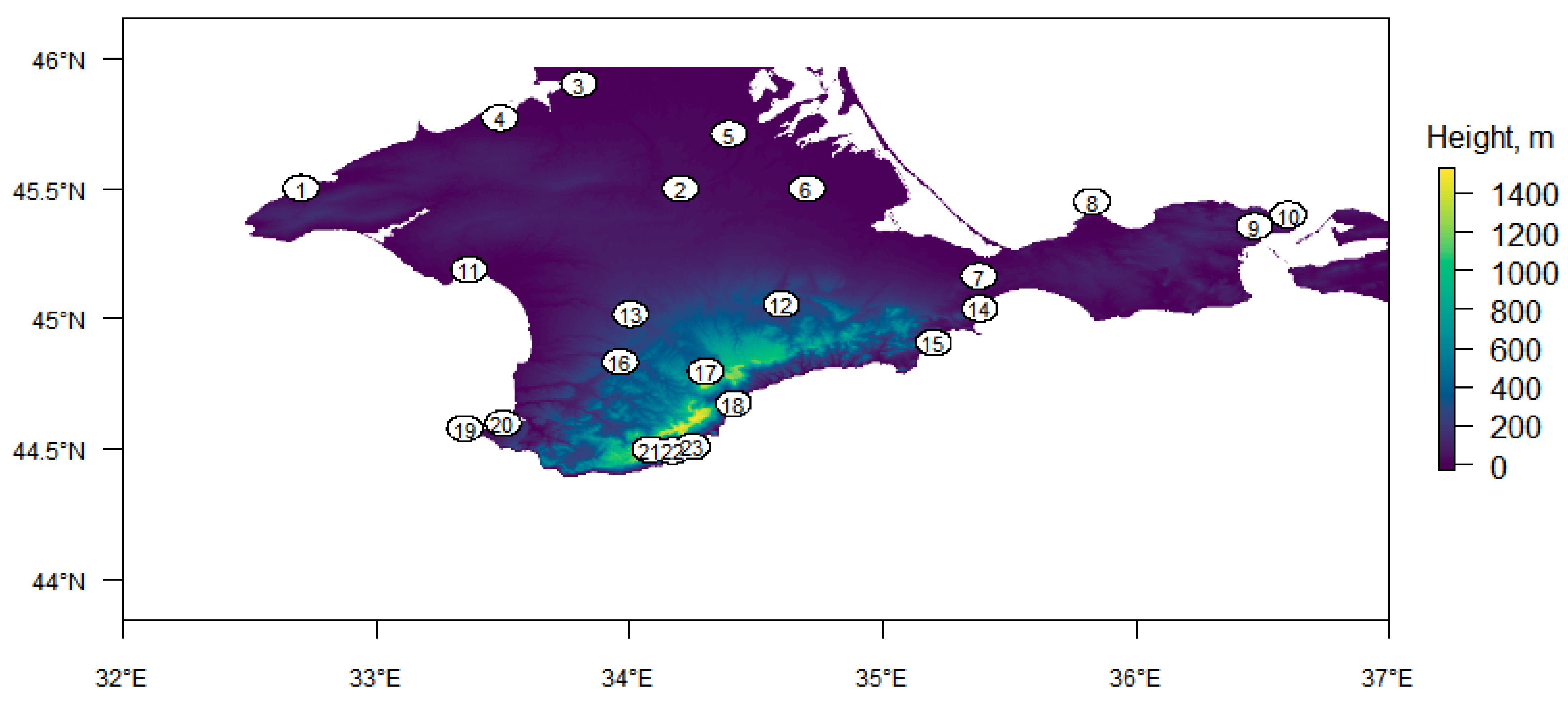
2.1. Study Area and Data

Crimea is situated to the north of the Black Sea region (between 32.3° E and 36.6° E in longitude and 44.35° N and 46.0° N in latitude). The region of Crimea is characterized by variety of terrain and landscapes and, hence, by pronounced meso- and micro-climatic features of hydrometeorological regime. The adjoining sea water area exerts a considerable influence on the climate in the coastal areas of Crimea and can be considered as one the main meso-climatic factors.

When studying SWP, it is crucial to choose an objective criterion for a meteorological phenomenon that poses a threat to citizens and/or a risk of damage within a region. When selecting criteria, the following conditions should be taken into account:

• The critical value of hydrometeorological quantity or intensity of the phenomenon must be rare for a given territory or time of year;
• The recurrence probability of the meteorological value associated with SWP should be no more than 10%.

Implementing these conditions implies the setting of thresholds for the meteorological values associated with SWP. The moment when the meteorological value starts to exceed the threshold is the beginning of SWP. The time interval of the threshold exceeding the meteorological value is the SWP duration. Data on the characteristics of SWP (SWP type and duration) at 23 meteorological stations in Crimea for the period 1976–2020 were used for the calculations (see

Table 1. List of meteorological stations of the Crimean region.

No.	Station Name	Code	Longitude, °	Latitude, °	Height, m	Data Available From
1	Chernomorskoe	4553270	32.703	45.502	9	1936
2	Klepinino	4553420	34.2	45.5	37	1936
3	Ishun	4593380	33.8	45.9	3	1959
4	Razdolnoe	4583350	33.487	45.77	16	1976
5	Dzhankoj	4573440	34.392	45.709	6	1944
6	Nizhnegorsk	4553470	34.7	45.5	19	1936
7	Vladislavovka	4523540	35.378	45.164	35	1959
8	Mysovoe	4553580	35.825	45.45	15	1936
9	Kerch	4543640	36.4673	45.3562	46	1955
10	Opasnoe	4543660	36.6	45.4	0	1955
11	Evpatoriya	4523340	33.366	45.19	2	1936
12	Belogorsk	4513460	34.599	45.057	205	1966
13	Simferopol	4503400	34.003	45.019	180	1936
14	Feodosiya	4503540	35.382	45.04	22	1936
15	Karadag	4493520	35.2	44.91	42	1937
16	Pochtovoe	4483390	33.963	44.836	172	1936
17	Angarskij pereval	4483430	34.3	44.8	765	1963
18	Alushta	4473440	34.41	44.6763	3	1936
19	Hersonesskij mayak	4463340	33.35	44.581	2	1936
20	Sevastopol	4463350	33.5	44.6	7	1936
21	Aj-Petri	4453410	34.1	44.5	1180	1936
22	Yalta	4453420	34.17	44.495	66	1936
23	Nikitskij sad	4453430	34.24	44.511	207	1936

and the geographical location in Figure 1). The period before 1976 was not taken into account due to heterogeneity (possible climatological heterogeneity [16] caused by the SWP observation method changing). Since 1976, the observations of SWP have been carried out between adjacent terms (0, 3, 6, 9, 12, 15, 18, and 21 h). On the contrary, before 1976, SWP were registered only in observational terms. The SWP dataset was subjected to a consistence check, which included procedures of intercomparison of the SWP record with records of relevant meteorological value. For example, SWP on precipitation must have coincided with high amounts of precipitation registered by a rain gauge.

SWP are a rather rare and intense phenomena evolution that is largely determined by local orography features. The methodology for studying SWP is limited by its rareness of occurrence and by substantial variability in time and space, which prevents a reliable assessment of SWP and its long-term variability [17]. Therefore, it is not recommended to carried out station-wise SWP analysis. Instead, one should make a report on SWP monitoring data aggregated for territories that are defined by physical-geographical, meso-climatic, or administrative features. We use the whole-region aggregation procedure to estimate the temporal variations of potential risks for regional economics arising from SWP. That is why station-scale data were preliminary aggregated into regional-scale data by attributing SWPs simultaneously occurring on a number of meteorological stations to one event of a regional SWP. Still, the reliability of the results of the method may remain debatable. In order to confirm the main conclusions of SWP analysis, we conducted a statistical estimation of extreme precipitation using non-stationary models (see Section 2.3). Statistical samples were formed from the maximum annual daily precipitation for each station in Table 1. Fifteen stations had quite long data series (since 1936–1937); for seven stations, data were available from 1950 to 1960. The exception was the Razdolnoe station, which has been operating since 1976. There are four stations in the Crimean Mountains and foothills viz. Aj-Petri, Angarskij pereval, Belogorsk, and Nikitskij sad.

The analysis of the synoptic processes of heavy precipitation indicated as SWP was carried out using an array of expert-prepared maps of a baric system’s features, enabling one to summarize the evolution and trajectories of near-surface cyclones and anticyclones for a long period. In addition, the analysis of large-scale atmospheric processes in the mid-troposphere (500 hPa) was carried out using the NCEP–NCAR Reanalysis 1 data set [18].

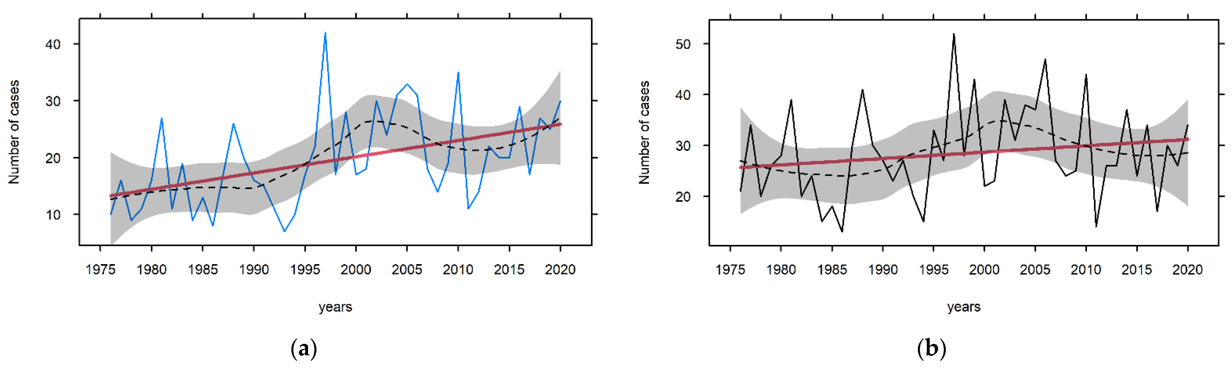
2.2. Time Series Analysis

A spectral analysis of time series was performed using the standard Daniell method [19]. The spectrum was calculated using the Tukey spectral window with effective degrees of freedom (df) of 6. Before the spectral analysis, the polynomial trend of the 2nd order was preliminary removed from the time series.

In the present study, the calculation of non-linear trends of interannual variability in the frequency of SWP was performed. The search for parametric regression y = X^Tβ can be considered as a classical problem of empirical risk minimization [20]. The optimal regression parameters β can be found using the following condition:

$$\widehat{\beta }=\underset{\beta ϵR^d}{\arg \min }{{\displaystyle \sum }}_{i=1}^{n}l\left(u_i,\beta \right)$$

where l(.) is the loss function (non-negative function with a single minimum), and u is the residual $u_i=y_i-x_i^T\beta$ between the value of the regression function and the empirical value of the dependent variable y_i. The least squares method (LSM) considers the loss function to be l(u) = u², and β characterizes the change in the average values y. This method can be used to estimate simple polynomial trends in hydrometeorological timeseries; however, if the trend function is complex and unknown in advance, the local polynomial regression method may be applied. The main idea here is that the trend function can be locally approximated by the polynomial of the p-th degree, using the Taylor series expansion in the vicinity of a local point x. When constructing a local polynomial, the following optimization problem is imposed [21]:

$$\underset{\beta ϵR^d}{\arg \min }{{\displaystyle \sum }}_{i=1}^n{\omega }_i\left(x\right)l\left(y_i-{\tilde{x}}_i^T\beta \right)$$

(1)

where ${\tilde{x}}_i^T=\left(1,\left(x_i-x\right),{\left(x_i-x\right)}^2,\dots ,{\left(x_i-x\right)}^p\right)$ and $\beta ={\left({\beta }_0,{\beta }_1,\dots ,{\beta }_p\right)}^T$ are related to local derivatives of the trend function at point x (corollary of the Taylor expansion). The greatest $\beta$ value is the coefficient β₀ standing for the value of the trend function at point x. Obtaining a set of β₀ values is a goal of local polynomial regression. The key component of Equation (1) is a limited kernel smoothing function $\omega \left(x\right)=K\left(x_i-x/h\right)$ with parameter h standing for the smoothing window width. In this paper, we have used symmetric Gaussian function as the kernel with the window width h = 5 years. Parameter h, along with a type of polynomial, describes the degree of smoothness of the trend function. Since the main objective of the study was to assess the long-term trends in meteorological timeseries, the h value was selected, not due to the objective criteria (e.g., randomness and independence of the regression residuals), but for filtering the high-frequency components of the climate series. A second-degree polynomial smoothing function was used, which is believed to reflect the non-linear structure of variability.

2.3. Statistical Estimation of Extremes

The study of statistical features of extreme precipitation was carried out using the block maxima method. As a rule, the block method uses annual maxima, the distribution of which, for large samples, follows one of three asymptotic distributions—Gumbel, Weibull, or Fréchet. In general, a probability function depends on the type and the parameters of the initial distribution of the meteorological value. However, if the probability distribution function is unknown, then it is recommended to use the generalized extreme value distribution function (GEV), as follows:

$$F_{GEV}\left(x\right)=Pr\left\{X\le x\right\}=exp\left[-{\left(1+\xi \cdot \frac{x-\mu }{\sigma }\right)}^{-\frac{1}{\xi }}\right]$$

(2)

where ξ, σ, and μ are the shape, scale, and location parameters, respectively. In order to estimate the parameters θ = (μ, ξ, σ), one can use the maximum likelihood method (MLM) [22] by maximizing the likelihood function $L\left(\theta ,y\right)={\displaystyle \prod }_{i=1}^{n}f\left(y_i|\theta \right)$, where $f\left(y_i|\theta \right)$ is the probability density function.

As a rule, the calculations are carried out under the assumption of constant θ. However, the non-stationarity of the time series that are used to extract the sample of extrema results in the time-dependence of the vector of parameters. This dependence can be approximated by the linear functions of covariant variables as follows:

$$\{\begin{array}{l}{\mu }_t={\displaystyle \sum }_{i=1}^k{\alpha }_i{U}_i\left(t\right)\\ \log {\sigma }_t={\displaystyle \sum }_{i=1}^k{\delta }_i{V}_i\left(t\right)\\ {\xi }_t={\displaystyle \sum }_{i=1}^k{\gamma }_i{W}_i\left(t\right)\end{array}$$

where U = (U₁, U₂, …, U_k), V = (V₁, V₂, …, V_k), and W = (W₁, W₂, …, W_k)—covariant variables, which in turn can be functions of time; α_i, δ_i, γ_i—hyperparameters; I = 1, …, k, k—number of covariates. The logarithm of σ was introduced to preserve positive values of the scale parameter, which plays the role of standard deviation.

In the non-stationary case, the likelihood function is represented as follows:

$$L_n={{\displaystyle \prod }}_{t=1}^n{f}_{GEV}\left(x_t|{\mu }_t,{\sigma }_t,{\xi }_t\right)$$

from which one can estimate the hyper-parameters of the distribution function.

However, it has been previously shown that the standard MLM is unstable on small samples (the most frequent case in practice) [23]. A more stable method is called the generalized maximum likelihood method (GMLM), which was also recommended in [23]. Stability is achieved by a priori parametrization of the distribution of the ξ parameter by beta function ${\pi }_{\xi }\left(\xi \right)=Beta\left(u=6, v=9\right)$. The parameters of the beta function were determined previously by treating a large array of geophysical data. In the framework of the GMLM, hyper-parameter estimates are the solution to the following optimization problem:

$$\{\begin{array}{l}\underset{\theta }{\max }{L}_n\left(x;\theta \right)\\ \xi ~Beta\left(u,v\right)\end{array}$$

which is equivalent to the maximization of the posterior distribution of hyper-parameters that are defined on an empirical sample by using $\pi \left(\theta |x\right)\propto L_n\left(x|\theta \right){\pi }_{\xi }\left(\xi \right)$. The search for the mode of this distribution and the corresponding parameter estimates can be performed by the gradient method, e.g., the Newton–Raphson method. All calculations were performed within the statistical programming environment R [24].

3. Hazard Meteorological Events in Crimea

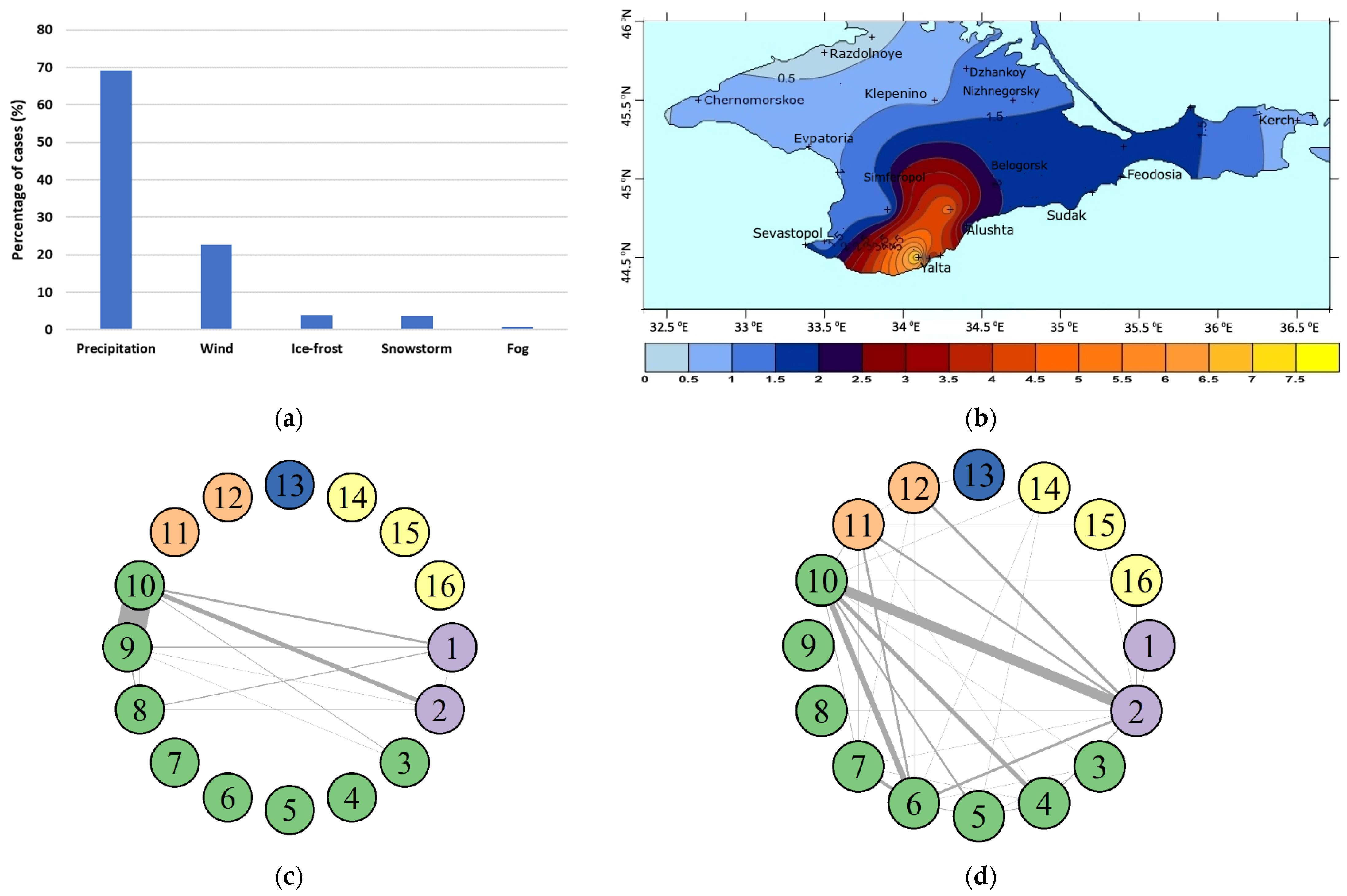
3.1. SWP of All Types on the Crimean Peninsula

The total amount of meteorological phenomena that reached the SWP criterion at one or more observational sites for 1976–2020 was 1254 events. These events were divided into 16 types of SWP, as follows: squall, strong wind, continuous heavy rain, sleet shower, sleet, snow shower, snow, hailstorm, torrential rain, heavy rain, general snowstorm (blizzard, snowstorm, drifting snow), blowing snow, fog, complex deposits, rime ice, and glaze ice. In order to simplify the presentation of the results, all of the types of SWP were combined into macrogroups called “precipitation”, “wind”, “ice-frost phenomena”, “snowstorm”, and “fog”.

The distribution of the number of cases for each type of SWP is depicted in Figure 2. In the Crimea macrogroup “precipitation” dominates in terms of the total proportion of cases of SWP (864 cases or ~69%). The SWP of strong wind also has a substantial contribution to the number of phenomena (22.4%), while other types of SWP have much less share; ice-frost phenomena account for 3.7% of SWP cases and snowstorms account for 4.4%. There were only eight cases of strong fog for the period 1976–2020. More frequently, SWPs were observed in the regions of the Crimean Mountains and the Southern Coast of Crimea (SCC). SWP are rare events in the steppe part of the Crimean Peninsula (Figure 2b). An obvious factor for the spatial distribution of SWP occurrence is the physical and geographical features of Crimea and the striking differences in the various forms of relief.

Regardless of the SWP type, their annual occurrence in Crimea is 27 events per year. A large group of SWPs is strongly related to a certain season (i.e., winter SWPs, such as blizzards, ice-frost phenomena, hail, snow, etc.). More frequently, SWPs are registered in summer (35.1%) and winter (33.7%); however, in autumn (18.1%) and spring (13.1%) such phenomena are observed much less frequently (Table 1). The maximum number of cases of SWP was registered in the summer of 1997 (27 cases) and in spring (13 cases). The largest number of SWPs in the winter season was registered in 2004 (19 cases), while autumn of 1981 turned out to be an “extreme” season (11 cases of SWPs).

The study of SWP of different types occurring at meteorological stations simultaneously that are triggered by the same synoptic process is of great scientific and practical interest. The analysis of the frequency of simultaneous SWPs has revealed that, in the majority of cases (about 84%), only one type of SWP was observed. In other cases, a complex of two to five SWPs of different types was recorded. The complex also included the cases when different types of SWP were observed at different stations. The SWP complex was observed in all months except April. The biggest group of SWPs (with different solid and liquid precipitation during a blizzard) was simultaneously registered on 2 January 1988; in the warm half-year it was on 29 August 2006 when convective phenomenon broke out, which were accompanied by heavy rain and strong wind. It should be noted that the above-mentioned combinations of the SWP types may occur only in certain half-years. Figure 2c,d illustrate half-year-dependent combinations of SWP as a result of SWP analysis for the whole period of 1976–2020. The thickness of the edges between the two vertices indicates a frequency of occurrence of a given combination. From Figure 2c,d one can draw a conclusion that “heavy rain/torrential rain” is more frequently combined with “strong wind/squall” SWPs in the warm half-year, while in the cold half-year, a combination of “rain/snow” with “strong wind” is more typical. In more than 5% of all of the SWPs events, heavy precipitation was indeed accompanied by an increase in wind speed up to the SWP criterion values, and most often this happened in the winter season. In summer, as a rule, short-term amplifications (of less than one hour) of wind (squall) occur during convective phenomena, which are accompanied by thunderstorm or/and hail. During complex “rain/wind” SWP phenomena, winds of southern and south-western directions were registered in the vast majority of cases (53% of cases of simultaneous SWP occurrence). From a synoptic viewpoint, this was probably due to the movement of the frontal boundary in front of a trough. For comparison, the predominant direction for all of the cases of very strong winds on the Crimean Peninsula is the northwest. According to Figure 2d, there are a number of cases of a “strong wind/snowstorm” combination. Only 7.2% of all of the SWPs of strong wind were accompanied by snowstorms, which at some sites reached the SWP criterion. Most often, this happened in January, with the prevailing northwestern wind direction.

3.2. SWP of Precipitation in Crimea

The SWP of precipitation consists of eight types of phenomena, which can be ranked by occurrence as follows: “heavy rain” (45.0%), “torrential rain” (9.2%), “hailstorm” (1.4%), “snow” (1.1%), “snow shower” (8.8%), “sleet” (1.0%), “sleet shower” (1.6%), and “continuous heavy rain” (0.3%). On average, about 19 cases of SWPp per year occur within the current climate period. SWPp are more likely to occur in the warm half-year (about 62%); however, in certain years, the SWPp occurrence in the cold half-year was higher (see

Table 2. Long-term averaged characteristics of SWP on the Crimean Peninsula using data of meteorological network for the period 1976–2020.

SWP Group	Month												Year
	January	February	March	April	May	June	July	August	September	October	November	December
Number of cases
Precipitation	71	53	34	14	48	128	133	133	70	52	39	69	844
Wind	51	43	32	15	6	14	9	10	8	19	26	44	277
Ice-frost phenomena	18	12	3	0	0	0	0	0	0	0	4	9	46
Blizzard	16	16	6	0	0	0	0	0	0	0	1	5	44
Fog	2	0	1	0	1	0	0	0	0	1	0	3	8
Average duration (time)
Precipitation	10.5	11.0	10.6	10.2	6.4	6.2	4.3	4.8	6.8	9.7	9.8	10.3	8.4
Wind	6.3	6.0	5.4	2.6	6.4	0.6	0.7	1.0	4.8	4.2	7.2	4.8	4.2
Ice-frost phenomena	40.6	45.9	9.9								26.3	48.1	34.2
Blizzard	21.6	22.1	19.7								18.2	20.4	20.4
Fog	38.1		25.0		20.2					21.1		24.6	27.0
Maximum duration (time)
Wind	35.2	26.9	26.8	6.1	12.0	17.5	2.8	3.3	12.5	13.6	34.0	23.6	35.2
Ice-frost phenomena	105.0	147.9	20.0								50.7	170.8	170.8
Blizzard	40.0	54.3	22.0								18.2	23.0	54.3
Fog	54.1		25.0		20.2					21.1		37.4	54.1

). In the summer, SWPp were observed twice as often as in the winter or the autumn; these events occur extremely rarely in the spring. The mean duration of SWPp was more than eight hours, though it has seasonal features. During the warmer months, the SWPp mean duration is shorter (minimum 4.3 h in July) while during the colder months it increases up to 11 h (Table 2). A few cases of super-intensive rainfall were registered, for example, in Klepinino on 18 September 2016, 33 mm of rain fell in just 22 min and in Belogorsk on 15 July 2006, 36.1 mm fell in 26 min.

In 63.6% of cases, SWPp were only registered at one of the monitoring sites in Crimea, in 20.9% of cases at two sites, and in 9.3% at three sites. SWPp registering at three or more sites at the same time is highly likely to occur in the summer or autumn. There were two extraordinary events when SWPp were recorded at 8 and 11 sites simultaneously—on 16 September 2002 and 23 September 2014, respectively.

Significantly more frequently, SWPp are observed in mountainous region of Crimea (224 cases in Aj-Petri) and SCC (106 cases in Yalta); however, precipitation is observed in the steppe region of the peninsula extremely rarely (only seven cases in Razdolnoe). One can put such a contrast in the number of cases of SWPs down to an influence of terrain relief on precipitation formation [25,26]. In particular, the precipitation depends on the height of the slopes, the horizontal dimensions of the uplands, the orientation, and the openness in relation to the moisture-carrying flow and general conditions of weathering. The Crimean Mountains contribute to the strengthening of the ascending air movements and the development of convection activating frontal boundary that is followed by intense torrential rain, thunderstorms, and strong wind.

In the mountainous region and SCC, the maximum of SWPp occurrence falls in the winter season (37% of cases in Yalta and more than 47% in Aj-Petri); however, for other regions of the Crimea, the maximum of SWPp occurrence is associated with the summer season. In summer, SWPp are caused by local fast-developing atmospheric processes that are associated with the formation of small but active convection cells. SWPp are the reason for river floods, landslides, and soil erosion. SWPp may be followed by hail, squall, and tornado, which can be dangerous for agricultural crops. It was on 5 June 2019 when similar unfavorable weather conditions were formed, inducing heavy rain and hail that damaged 3.5 thousand hectares of farmland.

Current climatology concerns the assessment of the sensitivity of extreme hydrometeorological phenomena to climate change—an issue that is of fundamental and practical interest [27]. The monotonous climatic trends in climate variables are believed to impose disproportionate “shifts” in the frequency and intensity of hazardous phenomena [28]. In order to assess the corresponding risks for Crimea, it is necessary to analyze the interannual variability in the frequency of SWPp.

The long-term variability of SWPp frequency has a significant (p-value < 1%) positive trend of 2.7 cases per decade (Figure 3). The trend in the annual frequency of SWPp also contributes to the long-term variability of SWP (with the positive trend being 1.3 cases per decade). It is worth noting that occurrence of other types of SWP does not significantly change the trend of SWP variability. The SWP annual frequency varies from 13 cases (1986) to 52 cases (1997). In order to characterize the variability in the SWP frequency, the coefficient of variation C_V was computed. For SWP, the C_V was 0.3 and for SWPp it was estimated to be 0.4. Such values of C_V indicate a moderate degree of variability of the SWP annual frequency. The smoothing of the time series by the local polynomial smoothing method enables one to conclude that the highest frequency of SWPp (or SWP) was observed in 1997–2007. Nevertheless, the interannual variability of SWPp (or SWP) annual frequency is irregular and features quasi-periodicity (Figure 3). The spectral analysis of the time series revealed the dominating fluctuations of SWPp annual frequency to have periods of four years and seven to nine years. The spectral structure of the SWP frequency time series is governed by the dynamics of SWPp, i.e., for the interannual variability of SWP, spectral peaks have been found to associate with the same time periods.

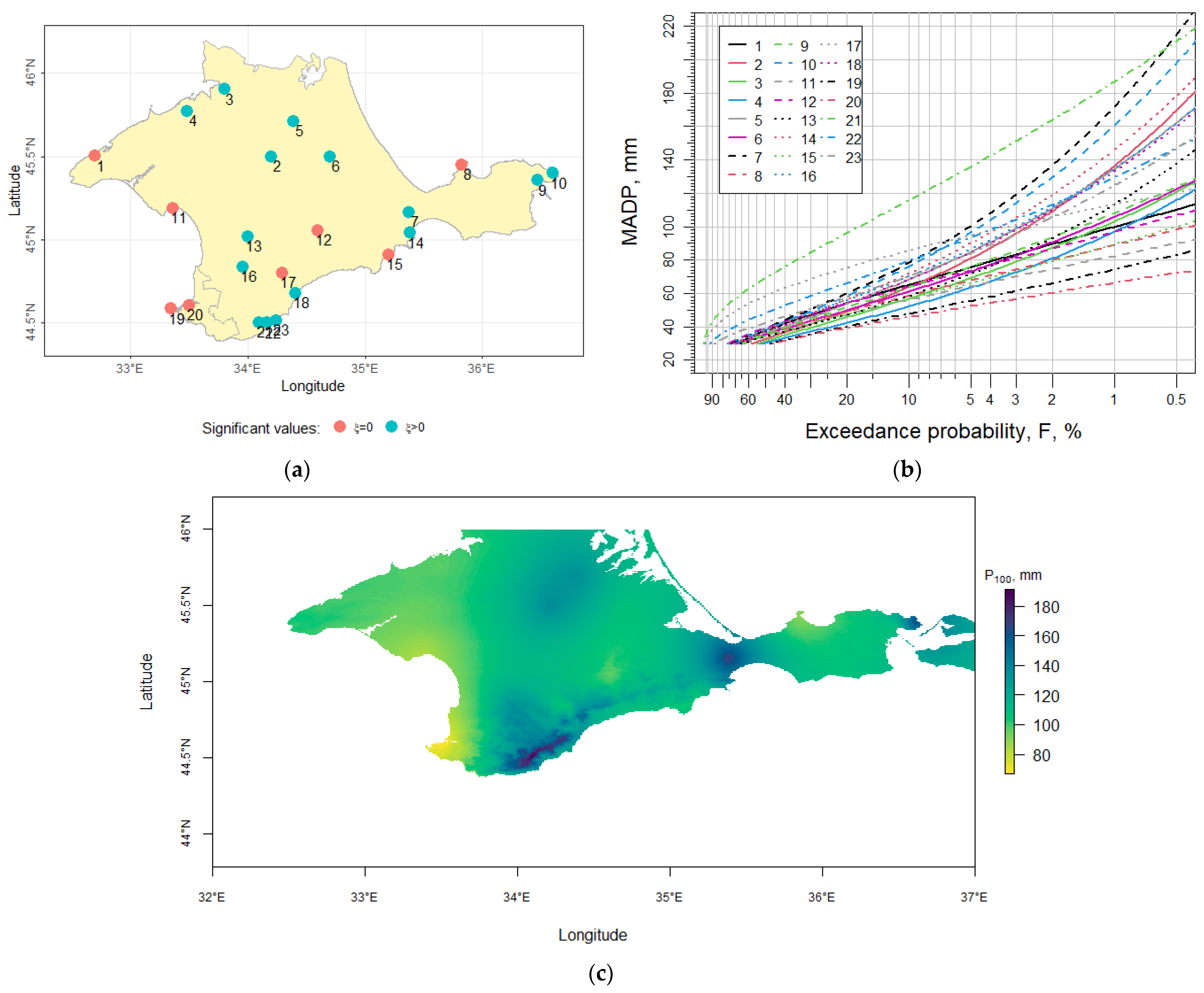
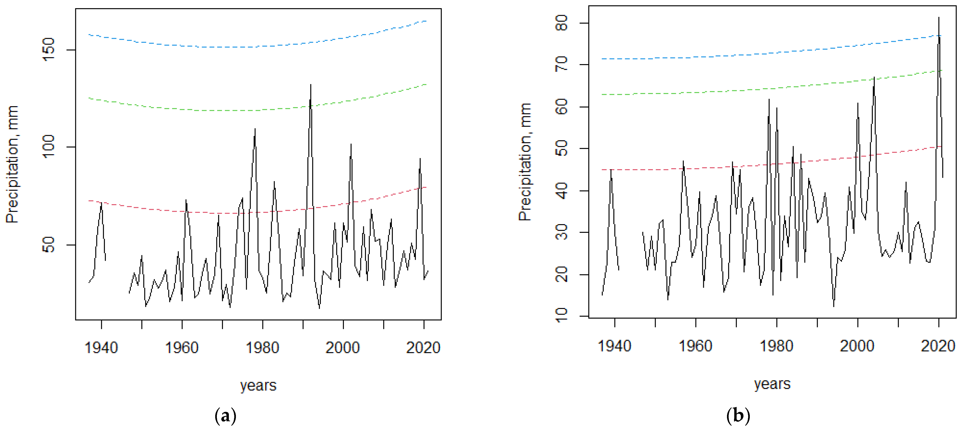
4. Statistical Analysis of Maximum Annual Daily Precipitation

4.1. Application of Stationary GEV Function

The block maxima method was used to sample the extreme daily precipitation for each meteorological station of Crimea. The sample sizes ranged from 44 to 80 values, depending on the gaps and the data availability (Table 1). The stationary GEV function was applied for the statistical modeling of the maximum annual daily precipitation (MADP). The GEV parameter estimation was carried out by the maximum likelihood method (see Section 2.3). Figure 3c plots the theoretical curves of the GEV function that are fitted to MADP samples for each station.

The Crimean Mountains stations Aj-Petri and Angarskij pereval were found to have the highest MADP return levels within the range of exceedance probability F(P) ≥ 8% (return period 12.5 years). For the exceedance probability F(P) < 5% (return period 20 years), station Aj-Petri, along with Opasnoe and the stations of the region of SCC, have the highest MADP return levels, estimated to be more than 150 mm, which is relevant to mountainous areas. On the contrary, the lowest estimates of return levels for MADP correspond to stations in western and southwestern Crimea. At these stations, the MADP for a return period of 100 years (MADP₁₀₀) do not exceed 100–105 mm (Figure 4c).

The fitted curves of the GEV function for the exceedance probability of MADP differ by its form (Figure 4b) and, consequently, by the theoretical model.

Table 3. GEV parameter estimates for annual maximum daily precipitation (mm).

No.	Station Name	GEV-Function Parameters Estimates
		Sample Size, L	μ0	σ	ξ
1	Chernomorskoe	78	32.3	14.6	0.004 *
2	Klepinino	80	28.5	11.1	0.295
3	Ishun	61	27.4	10.8	0.173
4	Razdolnoe	44	27.4	8.4	0.237
5	Dzhankoj	73	31.1	12.6	0.232
6	Nizhnegorsk	80	31.0	11.3	0.151
7	Vladislavovka	58	33.9	13.8	0.302
8	Mysovoe	77	30.5	12.4	0.011 *
9	Kerch	66	30.8	12.8	0.114
10	Opasnoe	60	32.8	14.0	0.271
11	Evpatoriya	80	30.1	11.9	−0.019 *
12	Belogorsk	77	34.5	12.8	0.023 *
13	Simferopol	80	30.6	9.0	0.276
14	Feodosiya	80	32.8	12.8	0.259
15	Karadag	70	30.5	10.9	0.069 *
16	Pochtovoe	79	34.2	12.2	0.234
17	Angarskij pereval	58	52.5	16.4	−0.078 *
18	Alushta	80	32.0	12.3	0.231
19	Hersonesskij mayak	80	26.0	9.0	0.066 *
20	Sevastopol	80	25.7	9.2	−0.015 *
21	Aj-Petri	79	60.9	22	0.093
22	Yalta	80	43.0	14.2	0.117
23	Nikitskij sad	80	38.1	11.2	0.211

Note: sign ‘*’ indicates an insignificant value for a parameter at a 95% confidence level.

gives the LSM estimates for the GEV parameters of Equation (2). The GEV is a generalization of three families of probability distributions of extreme values and the attraction of the empirical sample, which is determined by shape parameter ξ, as follows:

ξ > 0—Fréchet domain;

ξ = 0—Gumbel domain;

ξ < 0—Weibull domain.

According to Table 3, all but three of the stations have a positive ξ value. Moreover, for these three stations, three of the ξ values have a magnitude that is insignificantly different from 0 (95% confidence). Figure 4a illustrates the spatial distribution of the significant values of ξ.

In [29], a global analysis of the MADP was performed based on data from more than 15,000 meteorological stations covering the entire globe. According to the findings of this study, a true value of the shape parameter ξ, with a probability of 99%, can be found within the range of 0.0–0.23. In other words, the empirical distribution of MADP is attracted to the Fréchet domain of the GEV probability distribution function. Nevertheless, in our study sample, the values of ξ were exposed to scattering from negative (−0.098) to positive values (0.302). An explanation can be found in the same study [29], according to which the sample estimates of ξ are biased and depend both on the sample size L and the width of the confidence interval. Moreover, this dependence has the form of a power law function with the inverse exponent a + b × L^−c, that is, when sample size L increases, the accuracy of the ξ estimation also increases. It was found that, for a reliable statistical evaluation, no less than a 120-year-long time series would be required [29]. According to Table 1, the duration of the observations in Crimea does not exceed 85 years. A calculation using the numerical values of a, b, and c coefficients that are given in [29] and taking into account the available amount of data L (Table 3), led to the conclusion that all of the sample estimates of ξ for all of the Crimean stations fall into the theoretical 95% confidence interval with a true value of ξ > 0.

Papalexiou and Koutsoyiannis (2013) plotted the geographical distribution of the ranges of ξ where the Crimean region is characterized by a range of values of 0.00–0.10 [29]. However, in our study, the spatial distribution of the ξ values turned out to be different (Figure 4a). For most of the stations ξ was >0.1, for four stations ξ was <0, and only three of the stations strictly fell into the range [0.00; 0.10]. In contrast to [29], we used the data for all of the meteorological stations in the region. In addition, the equation for taking into account the bias of ξ that was proposed in [29] can be applied only to L-moment estimates [30].

4.2. Application of Non-Stationary GEV Function

The statistical features of meteorological extremes may vary between different periods of quasi-stationary climate. For example, a significant difference may exist between two adjacent standard climate periods of 1961–1990 and 1991–2020, though the latter is believed to be non-stationary with regard to the meteorological elements. The presence of non-stationarity in the time series can affect the reliability of the sample estimates to be obtained. Figure 5 depicts interannual variability of the MADP for two meteorological stations. Taking a look at the chart, one may infer a conclusion that the time structure of the series contains trend components, which, in a first approximation, can be described by simple polynomials.

It should be noted that the presence of a trend is primarily a characteristic feature of the air temperature regime in recent decades. Thus, empirical data indicate trends towards an increase in air temperature by an average of 0.8 °C since the beginning of the 20th century for most regions of Earth, which is considered to be a manifestation of global warming [1]. For the territory of Europe and the European territory of Russia, over the past 60–70 years, there has been an increase in the maximum, the minimum, and the daily mean air temperature in the cold season [4]. For the Black Sea region, there is also a steady trend towards climate warming, although the change in the surface air temperature from season to season is uneven [31], and the most striking trend is noted for the air temperature of the cold months of the year. In addition, statistically significant trends can be traced in other hydrometeorological characteristics. According to the long-term data of the coastal stations in the Black Sea region, there is a decrease in the average annual surface wind speeds [32], which is also supported by short-term satellite scatterometer data for the last two decades [33]. The regional wind velocity decrease is consistent with the widespread decrease in wind speed in the second half of the 20th century throughout the northern hemisphere [34]. The wave characteristics in the coastal zone of the Black Sea also show pronounced multidecadal variability, which is a manifestation of global climate trends [11].

The emergence of the non-stationarity of hydrometeorological series is a consequence of the slow evolution of large-scale processes in the global climate system and their manifestations at a regional level. The factor of climatic non-stationarity of the series influences the reliability of the statistical estimation of the extremes of precipitation when using marginal distributions. In our study, we calculated the extreme precipitation statistics using a non-stationary GEV model, assuming the time dependence of the location parameter μ as follows:

$$\mu \left(t\right)={\mu }_0+{\mu }_{1}t+{\mu }_2{t}^2$$

(3)

The calculation for the Crimean meteorological stations shows that, for 12 out of the 23 stations, the non-stationary location parameter μ in the GEV model turned out to be significant at the 95% confidence level. Examples of a non-stationary estimate of the MADP are presented in Figure 5 for two stations—Feodosiya and Hersonesskij mayak. According to Figure 5, during recent decades the probability of extreme precipitation has increased, at least in the vicinity of the two given stations. An example of torrential rain on 7 June 2019, favors this conclusion. During this event, the daily amount of precipitation at the Hersonesskij mayak station (81.3 mm) resulted in the registration of the record-breaking daily precipitation amount, which was the highest value since 1936.

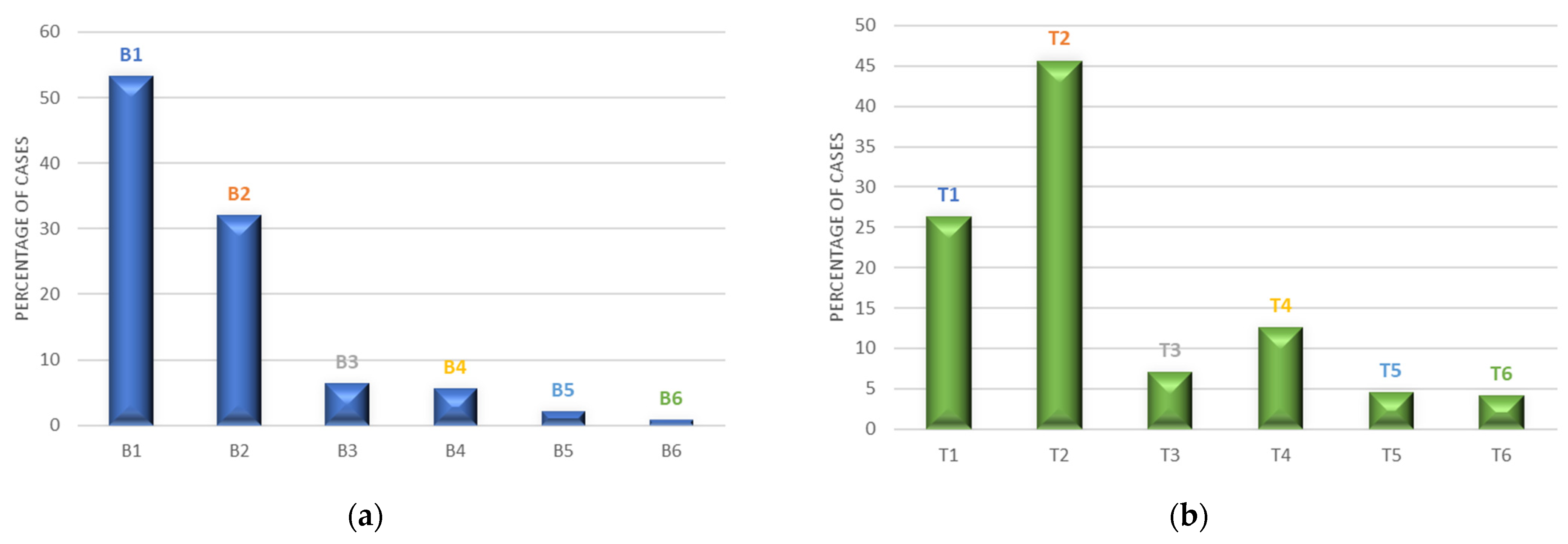
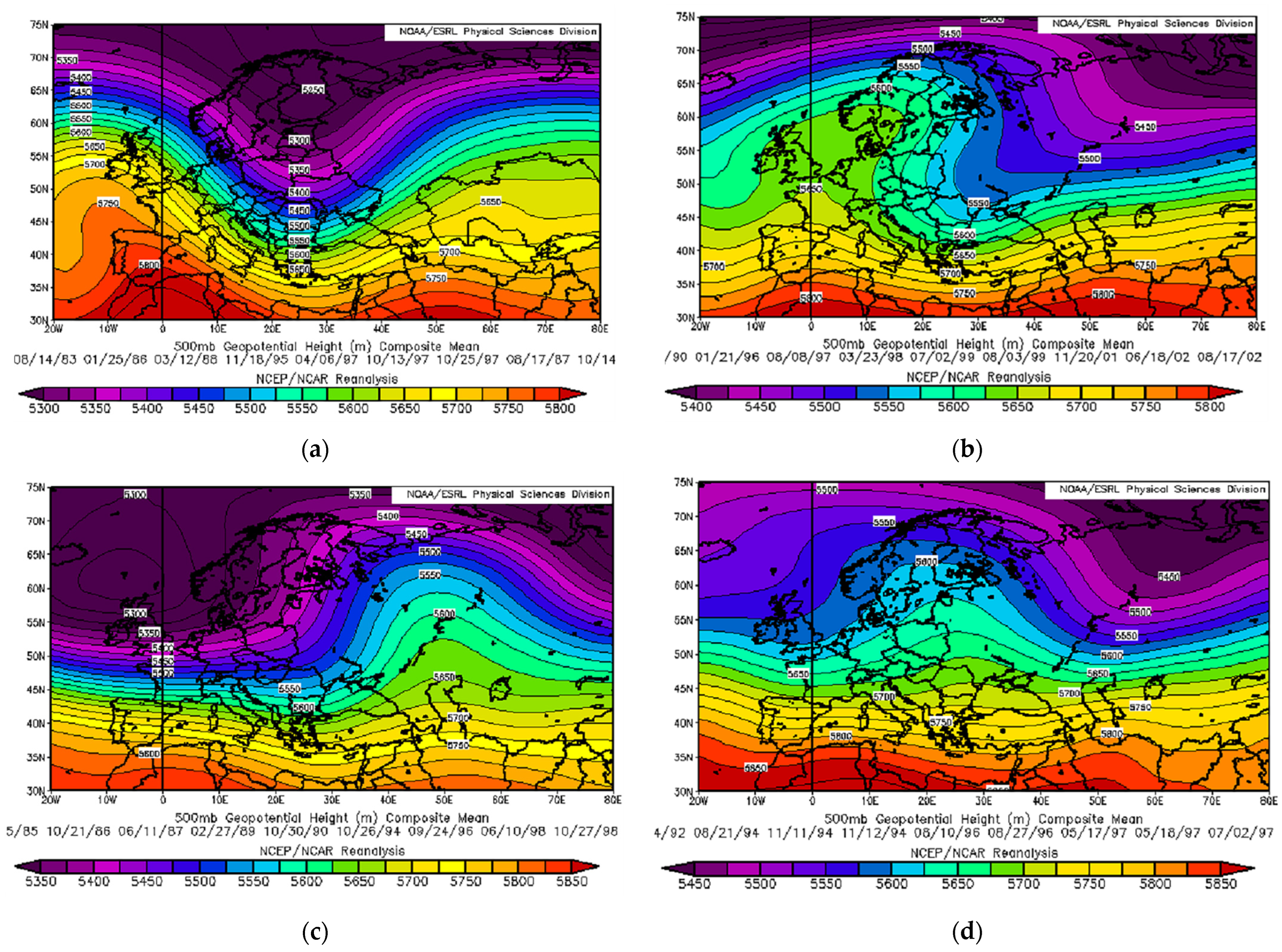
5. Atmospheric Trigger for SWPp

Despite the small-scale dimensions, the Black Sea region has a complex genesis of storm weather conditions that are associated with atmospheric processes transformation due to the active interaction of circulation systems of temperate and subtropical latitudes, as well as with the influence of the mountain systems of Caucasus and Crimea. Along with dominating west-eastern transport, which brings warm air masses from the Atlantic, mesoscale cyclogenesis over the Mediterranean and the Black Sea basins is an equally significant factor of weather formation in the region [35,36,37]. This influence is especially strong in the winter months of the year. The Black Sea is considered to be one of the most active areas of cyclone generation in Europe, which is due to the interaction of the circulation system of the Atlantic–European sector with the local orography of the region [37]. One of the apparent consequences of cyclogenesis is a formation of stormy weather conditions in the region.

The study of synoptic processes causing SWPp in Crimea was carried out by summarizing 689 cases of SWPp that were registered at meteorological stations during the period of 1976–2020. SWP synoptic processes were divided onto the following groups: southern cyclones, trough, northwestern cyclones, Atlantic cyclones, cyclones over Ukraine, and ridge. The synoptic process group occurrence is illustrated in Figure 6a. Some cases could not be attributed to any of the groups, which, apparently, may be due to the limited possibilities of expert evaluation. In the vast majority of situations, heavy precipitation was due to the movement of southern cyclones (more than 53%). Having enormous energy reserves, the southern cyclones can cause extreme weather conditions both in the Black Sea basin and in the Mediterranean [35,36,37]. A fairly large group of cases (about 32%) were caused by troughs, in front of which, as a rule, a frontal boundary is located. Other groups are represented by a significantly lower frequency of no more than 6%. The contribution of the northwestern cyclones is insignificant (6.2%). In Crimea, these cyclones are also associated with extreme ice-frost phenomena and snowstorms. A comparable number of SWPp was associated with the emergence of cyclones over Ukraine (5.6% of SWPp events), which also move along the northwestern trajectories, but cannot be attributed to the northwestern cyclones based on the mechanism of its genesis. Extremely rarely SWPp were caused by the movement of Atlantic cyclones (0.8%), which typically induce strong winds.

Thus, the southern cyclones make the greatest contribution to the formation of hazardous SWPp in the region. It is interesting to note that in about half of all of the cases of SWPp that were caused by southern cyclones (47.9%), the main region of cyclogenesis was the Black Sea basin in all seasons except winter. At the same time, the Black Sea cyclone cases are mostly local (mesoscale), are small in area, and are short-lived cyclones that are traceable for 3–9 h. The maximum frequency of cyclogenesis in the Black Sea occurs in its eastern part throughout the year, intensifying in July and August [38,39]. The next areas of southern cyclone genesis are the Aegean Sea (12.1%), the Balkan Peninsula (9.7%), and the Adriatic Sea (9.2%). The contribution of the other regions is much less.

The movement of the northwestern cyclones on the Black Sea coast most often (50.0% of all of the cases of northwestern cyclones causing SWPp) occurred from the areas of the Baltic Sea; such cyclones moved from the Barents Sea and Iceland less often (3.5%).

The origin and the development of cyclones occurs under the influence of leading large-scale processes in the free atmosphere, for example, the disturbance of a global eastward transport and the formation of a meridional high-altitude frontal zone [40]. Furthermore, the analysis of the atmospheric processes in the middle troposphere according to the data on the 500 hPa geopotential height from the NCEP-NCAR reanalysis has been carried out. The array of daily geopotential height fields was compiled from the set of dates of SWPp. The SWPp dates were divided into four large groups of cases that were unified by the similarity of the synoptic processes in the middle troposphere (Figure 6b). These groups were designated as “mixed”, “western”, “eastern”, and “central”. For each group, a composite analysis was conducted, the result of which is illustrated in Figure 7. Each composite in Figure 7 reflects the development of the meridional form of large-scale atmospheric circulation. The west-east (zonal) transport of air masses rarely induces hazardous phenomena in the Crimean region (4.5%). In some cases (4.1%) the synoptic processes could not be attributed to any of the presented groups.

5.1. “Mixed” Group

During the development of SWPp in Crimea, a deep high-altitude trough occurs more frequently (about 45%) in the middle troposphere above the Black Sea basin (Figure 7a). Well-developed high-altitude ridges can be traced over Western Europe and Western Siberia, one of which is directed from the Mediterranean Sea to Scandinavia (Norwegian Sea), and the other to the eastern part of the European territory of Russia. Depending on the localization of the ridges, with respect to the Black Sea basin, the transfer of the air masses to the Black Sea in one case is carried out from the south or the south-west (14.3%) and in other cases from the north or the north-west (8.6%). Quite often (17.8%) an isolated high-altitude cyclone was identified above a deep trough over the Black Sea basin.

5.2. “Western” Group

The “western” group contains cases with a well-defined ridge (about 26%) that are oriented from the west of the Mediterranean to the British Isles or Western Europe (5.0%), as well as those cases where a well-developed ridge of subtropical anticyclone was oriented in the east (north-east) direction, from the regions of the Azores to Scandinavia and the western regions of the Kara Sea (6.8%) (Figure 7b). A number of cases occurred when an isolated high-altitude cyclone (13.2%) was observed near the Black Sea basin. Here, warm air masses are transported towards the north along the western periphery of the low regions. At the same time, the Arctic Sea air masses spread to the central and southern regions of the European territory along eastern periphery of the low regions.

5.3. “Eastern” Group

During the eastern localization of the high-altitude ridge, SWPps can be induced in 12.5% of cases, and in almost half of the cases (6.4%), an isolated high-altitude cyclone was traced near to the Black Sea basin (Figure 7c). A characteristic feature of this group is the absence of an ultra-polar invasion of the Arctic air to the European continent along the ultra-polar trajectory (from the north or the north-east to European Russia).

5.4. “Central” Group

The atmospheric processes of the “central” group (7.0%) are featured by a vast area of high pressure in the middle troposphere (500 hPa) that is formed in the masses of the continental arctic air (Figure 7d). As in the two previous groups, in more than half of the cases, an isolated high-altitude cyclone can be traced over the Black Sea basin.

6. Conclusions

In this study we have shown that SWP frequency in Crimea is equal to 27 events per year (for 1976–2020). SWP are rather rare and intense phenomena, for which the evolution is largely determined by local orography features. That is why the spatial distribution of SWP occurrence is uneven, indicating the regions of the Crimean Mountains and SCC as a zone with much more frequent SWP (five to seven times higher in comparison to the steppe part of Crimea). Up to two-thirds of all of the SWP cases in Crimea are related to extreme precipitation SWPp. Therefore, extreme precipitation is the main threat for the region, which can cause high damage to its infrastructure and its economics. Moreover, this threat is still increasing. The annual frequency of SWPp has a significant (p-value < 1%) positive trend of 2.7 cases per decade. It is worth noting that interannual variability of SWPp annual frequency has dominating fluctuations with periods of four years and seven to nine years. In principle, the non-stationarity of the time series may influence the estimation of the statistical extremes of the precipitation amount, which plays a crucial role in the design of the drainage and sewerage systems in urban areas. We have implemented a non-stationary GEV model in order to estimate MADP for different return periods. The calculations have revealed the fact that, for at least 12 out of the 23 stations of the Crimean region, the non-stationary location parameter μ in the GEV model turned out to be significant at the 95% confidence level. Moreover, for these 12 stations, the probability of the occurrence of extreme MADP has increased. Thus, climate-induced non-stationary in the time series should be taken into account in dangerous hydrometeorological phenomena risk analysis.

The analysis of the synoptic near-surface processes of 689 cases of SWPp in Crimea revealed the fact that the greatest contribution to the formation of SWPp in the region is made by Mediterranean–Black Sea cyclones. For all seasons, except winter, in about half of all of the cases of SWPp the main region of cyclogenesis was the Black Sea basin. The contribution of the northwestern and Atlantic cyclones to the occurrence of the SWPp in Crimea is not significant. The analysis of the mid-troposphere circulation over the Atlantic–European sector allowed us to identify four types of meridional circulation that are associated with SWPp events. It should be mentioned that more than 42% of SWPp cases were accompanied by an isolated high-altitude cyclone in the mid-troposphere over the Black Sea region.

References

1. IPCC. Climate Change 2022: Impacts, Adaptation, and Vulnerability. Contribution of Working Group II to the Sixth Assessment Report of the Intergovernmental Panel on Climate Change; Pörtner, H.-O., Roberts, D.C., Tignor, M., Poloczanska, E.S., Mintenbeck, K., Alegría, A., Craig, M., Langsdorf, S., Löschke, S., Möller, V., et al., Eds.; Cambridge University Press: Cambridge, UK; New York, NY, USA, 2022; 3056p. [Google Scholar] [CrossRef]
2. Coumou, D.; Robinson, A. Historic and future increase in the global land area affected by monthly heat extremes. Environ. Res. Lett. 2013, 8, 034018. [Google Scholar] [CrossRef]
3. Zampieri, M.; D’Andrea, F.; Vautard, R.; Ciais, P.; de Noblet-Ducoudre, N.; Yiou, P. Hot European Summers and the Role of Soil Moisture in the Propagation of Mediterranean Drought. J. Clim. 2009, 22, 4747–4758. [Google Scholar] [CrossRef]
4. Caesar, J.; Alexander, L.; Vose, R. Large-scale changes in observed daily maximum and minimum temperatures: Creation and analysis of a new gridded data set. J. Geophys. Res. 2006, 111, D05101. [Google Scholar] [CrossRef]
5. Feudale, L.; Shukla, J. Influence of sea surface temperature on the European heat wave of 2003 summer. Part I: An observational study. Clim. Dyn. 2011, 36, 1691–1703. [Google Scholar] [CrossRef]
6. Donat, M.G.; Alexander, L.V.; Yang, H.; Durre, I.; Vose, R.; Dunn, R.J.H.; Willett, K.M.; Aguilar, E.; Brunet, M.; Caesar, J. Updated analyses of temperature and precipitation extreme indices since the beginning of the twentieth century: The HadEX2 dataset. J. Geophys. Res. Atmos. 2013, 118, 2098–2118. [Google Scholar] [CrossRef] [Green Version]
7. Coumou, D.; Rahmstorf, S. A decade of weather extremes. Nat. Clim. Chang. 2012, 2, 491–496. [Google Scholar] [CrossRef]
8. Mishra, V.; Ganguly, A.R.; Nijssen, B.; Lettenmaier, D.P. Changes in observed climate extremes in global urban areas. Environ. Res. Lett. 2015, 10, 024005. [Google Scholar] [CrossRef]
9. Hodnebrog, O.; Marelle, L.; Alterskjær, K.; Wood, R.R.; Ludwig, R.; Fischer, E.M.; Richardson, T.B.; Forster, P.M.; Sillmann, J.; Myhre, G. Intensification of summer precipitation with shorter time-scales in Europe. Environ. Res. Lett. 2019, 14, 124050. [Google Scholar] [CrossRef]
10. Chen, Y.; Liao, Z.; Shi, Y.; Li, P.; Zhai, P. Greater flash flood risks from hourly precipitation extremes preconditioned by heatwaves in the Yangtze River Valley. Geophys. Res. Lett. 2022, 49, e2022GL099485. [Google Scholar] [CrossRef]
11. Polonsky, A.; Evstigneev, V.; Naumova, V.; Voskresenskaya, E. Low-frequency variability of storms in the northern Black Sea and associated processes in the ocean-atmosphere system. Reg. Environ. Chang. 2014, 14, 1861–1871. [Google Scholar] [CrossRef]
12. The Global Risks Report 2022, 17th Edition, World Economic Forum. Available online: https://www.weforum.org/reports/global-risks-report-2022 (accessed on 15 August 2022).
13. Ullah, I.; Saleem, F.; Iyakaremye, V.; Yin, J.; Ma, X.; Syed, S.; Hina, S.; Asfaw, T.G.; Omer, A. Projected changes in socioeconomic exposure to heatwaves in South Asia under changing climate. Earth’s Future 2022, 10, e2021EF002240. [Google Scholar] [CrossRef]
14. Liu, Y.; Chen, J.; Pan, T.; Liu, Y.; Zhang, Y.; Ge, Q.; Ciais, P.; Penuelas, J. Global socioeconomic risk of precipitation extremes under climate change. Earth’s Future 2020, 8, e2019EF001331. [Google Scholar] [CrossRef] [PubMed]
15. Iyakaremye, V.; Zeng, G.; Yang, X.; Zhang, G.; Ullah, I.; Gahigi, A.; Vuguziga, F.; Asfaw, T.G.; Ayugi, B. Increased high-temperature extremes and associated population exposure in Africa by the mid-21st century. Sci. Total Environ. 2021, 790, 148162. [Google Scholar] [CrossRef] [PubMed]
16. Aguilar, E.; Auer, I.; Brunet, M.; Peterson, T.C.; Wieringa, J. Guidelines on Climate Metadata and Homogenization; WMO-TD No.1186, WCDMP No.53; WMO: Geneva, Switzerland, 2003; 55p. [Google Scholar]
17. Bedritskii, A.I.; Korshunov, A.A.; Shaimardanov, M.Z. The bases of data on hazardous hydrometeorological phenomena in Russia and results of statistical analysis. Russ. Meteorol. Hydrol. 2009, 34, 703–708. [Google Scholar] [CrossRef]
18. Kistler, R.; Kalnay, E.; Collins, W.; Saha, S.; White, G.; Woollen, J.; Chelliah, J.; Ebisuzaki, W.; Kanamitsu, M.; Kouksy, V.; et al. The NCEP-NCAR 50-year reanalysis: Monthly means CD-ROM and documentation. Bull. Am. Meteorol. Soc. 2001, 82, 247–267. [Google Scholar] [CrossRef]
19. Brockwell, P.J.; Davis, R.A. Time Series: Theory and Methods, 2nd ed.; Springer: New York, NY, USA, 1991; 580p. [Google Scholar]
20. Shibzukhov, Z.M.; Dimitrichenko, D.P.; Kazakov, M.A. The empirical risk minimization principle based on average loss aggregating functions for regression problems. Softw. Syst. 2017, 2, 180–186. [Google Scholar] [CrossRef]
21. Ghouch, A.; Genton, M. Local Polynomial Quantile Regression with Parametric Features. J. Am. Stat. Assoc. 2009, 104, 1416–1429. [Google Scholar] [CrossRef]
22. Coles, S. An Introduction to Statistical Modeling of Extreme Values; Springer: New York, NY, USA, 2001; 211p. [Google Scholar]
23. El Adlouni, S.; Ouarda, T.B.M.J.; Zhang, X.; Roy, R.; Bobèe, B. Generalized maximum likelihood estimators for the nonstationary generalized extreme value model. Water Resour. Res. 2007, 43, W03410. [Google Scholar] [CrossRef]
24. The R Project for Statistical Computing. Available online: http://www.r-project.org/ (accessed on 15 August 2022).
25. Gu, W.; Zhu, X.; Meng, X.; Qiu, X. Research on the Influence of Small-Scale Terrain on Precipitation. Water 2021, 13, 805. [Google Scholar] [CrossRef]
26. Paik, K.; Kim, W. Simulating the evolution of the topography-climate coupled system. Hydrol. Earth Syst. Sci. 2021, 25, 2459–2474. [Google Scholar] [CrossRef]
27. Hansen, J.; Sato, M.; Ruedy, R. Perception of climate change. Proc. Natl. Acad. Sci. USA 2012, 109, E2415–E2423. [Google Scholar] [CrossRef] [PubMed] [Green Version]
28. Trenberth, K.E. Framing the way to relate climate extremes to climate change. Clim. Chang. 2012, 115, 283–290. [Google Scholar] [CrossRef] [Green Version]
29. Papalexiou, S.M.; Koutsoyiannis, D. Battle of extreme value distributions: A global survey on extreme daily rainfall. Water Resour. Res. 2013, 49, 187–201. [Google Scholar] [CrossRef]
30. Hosking, J.R.M. L-moments: Analysis and estimation of distributions using linear combinations of order statistics. J. R. Stat Soc. Ser. B 1990, 52, 105–124. [Google Scholar] [CrossRef]
31. Evstigneev, V.P.; Naumova, V.A.; Evstigneev, M.P.; Lemeshko, N.A. Physiographic factors of seasonal distribution of linear trends in air temperature on the Azov-Black Sea coast. Russ. Meteorol. Hydrol. 2016, 41, 19–27. [Google Scholar] [CrossRef]
32. Evstigneev, V.P.; Lemeshko, N.A.; Naumova, V.A.; Evstigneev, M.P. Climate change induced uncertainty of wind energy potential for the Azov and Black Seas coastal zone. Ecol. Saf. Coast. Shelf Zones Sea 2020, 4, 22–39. [Google Scholar] [CrossRef]
33. Kubryakov, A.; Stanichny, S.; Shokurov, M.; Garmashov, A. Wind velocity and wind curl variability over the Black Sea from QuikScat and ASCAT satellite measurements. Remote Sens. Environ. 2019, 224, 236–258. [Google Scholar] [CrossRef]
34. Vautard, R.; Cattiaux, J.; Yiou, P.; Thépaut, J.N.; Ciais, P. Northern Hemisphere atmospheric stilling partly attributed to an increase in surface roughness. Nat. Geosci. 2010, 3, 756–761. [Google Scholar] [CrossRef]
35. Kaznacheeva, V.D.; Shuvalov, S.V. Climatic characteristics of Mediterranean cyclones. Russ. Meteorol. Hydrol. 2012, 37, 315–323. [Google Scholar] [CrossRef]
36. Nissen, K.M.; Leckebusch, G.C.; Pinto, J.G.; Renggli, D.; Ulbrich, S.; Ulbrich, U. Cyclones causing wind storms in the Mediterranean: Characteristics, trends and links to large-scale patterns. Nat. Hazards Earth Syst. Sci. 2010, 10, 1379–1391. [Google Scholar] [CrossRef]
37. Maslova, V.N.; Voskresenskaya, E.N.; Lubkov, A.S.; Yurovsky, A.V.; Zhuravskiy, V.Y.; Evstigneev, V.P. Intensive cyclones in the Black Sea region: Change, variability, predictability and manifestations in the storm activity. Sustainability 2020, 12, 4468. [Google Scholar] [CrossRef]
38. Ivanov, A.Y. Mesoscale Atmospheric Cyclonic Vortices over the Black and Caspian Seas as Seen in Satellite Remote Sensing Data. Izv. Atmos. Ocean. Phys. 2018, 54, 1089–1101. [Google Scholar] [CrossRef]
39. Yarovaya, D.A.; Efimov, V.V. Mesoscale cyclones over the Black Sea. Russ. Meteorol. Hydrol. 2014, 39, 378–386. [Google Scholar] [CrossRef]
40. Trigo, I.F.; Bigg, G.R.; Davies, T.D. Climatology of Cyclogenesis Mechanisms in the Mediterranean. Mon. Weath. Rev. 2002, 130, 549–569. [Google Scholar] [CrossRef]
Figure 1. Current network of meteorological stations in the Crimean region. Numbering of stations corresponds to the serial number in Table 1.
Atmosphere 13 01712 g001
Figure 2. Distribution of the number of cases of SWP by groups of SWP types (a), by the space of the Crimean region (b), graphs of combinations of SWP types of the warm (c) and cold (d) half-year according to data for the period 1976–2020. The color of the graphs corresponds to the SWP groups as follows: green—the “precipitation” group, purple—“wind”, yellow—“icy frost”, brown—“blizzard”, blue—“fog”. The numbers on the graphs correspond to the type of SWP as follows: 1—squall, 2—strong wind, 3—continuous heavy rain, 4—sleet shower, 5—sleet, 6—snow shower, 7—snow, 8—hailstorm, 9—torrential rain, 10—heavy rain, 11—general snowstorm (blizzard, snowstorm, drifting snow), 12—blowing snow, 13—fog, 14—complex deposits, 15—rime ice, 16—glaze ice.
Atmosphere 13 01712 g002
Figure 3. Long-term variability in the frequency of (a) SWPp and (b) SWP in Crimea for 1976–2020. The red line depicts a linear trend and the black dotted line and the grey-filled area are local polynomial smoothing and corresponding 95%-confidence region, respectively.
Atmosphere 13 01712 g003
Figure 4. Spatial distribution of shape parameter ξ (a), theoretical curves of GEV exceedance probability (F,%) for MADP (mm) (b), and interpolated MADP100 (c) using data of 23 meteorological stations in Crimea for 1936–2020. The numbers of points and lines coincide with the numbering of the stations in Table 1.
Atmosphere 13 01712 g004
Figure 5. Interannual variability of MADP and non-stationary estimates of MADP of different return periods for stations Feodosiya (a) and Hersonesskij mayak (b). Dashed lines of red, green, and blue color represent non-stationary estimates of MADP for return periods of 10, 50, and 100 years, respectively.
Atmosphere 13 01712 g005
Figure 6. Frequency of (a) baric objects and (b) types of atmospheric processes in the middle troposphere (500 hPa) according to SWPp data in Crimea for the period of 1976–2020: B1—southern cyclones, B2—trough, B3—northwestern cyclones, B4—cyclones over Ukraine, B5—undefined, B6—Atlantic cyclones; T1—western, T2—mixed, T3—central, T4—eastern, T5—zonal, T6—undefined.
Atmosphere 13 01712 g006
Figure 7. Composites of baric fields in the middle troposphere (500 hPa) during SWPp in the Crimean region: (a) mixed, (b) western, (c) eastern, and (d) central. Plots were built at Physical Sciences Laboratory (NOAA) site http://www.esrl.noaa.gov/psd/.
Atmosphere 13 01712 g007