
Estimation of Short-Term and Long-Term Ozone Exposure Levels in Beijing–Tianjin–Hebei Region Based on Geographically Weighted Regression Model
 ,
,
Abstract
:1. Introduction
2. Data and Methods
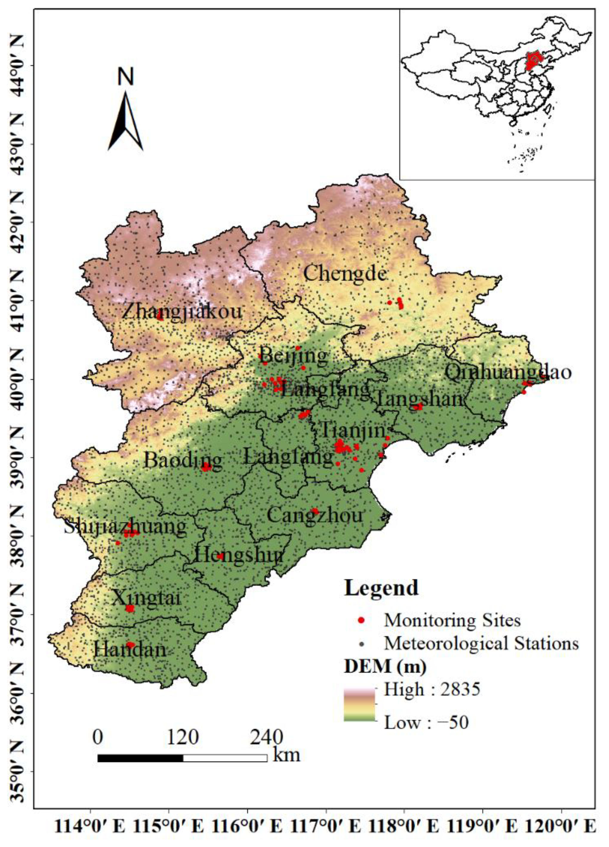
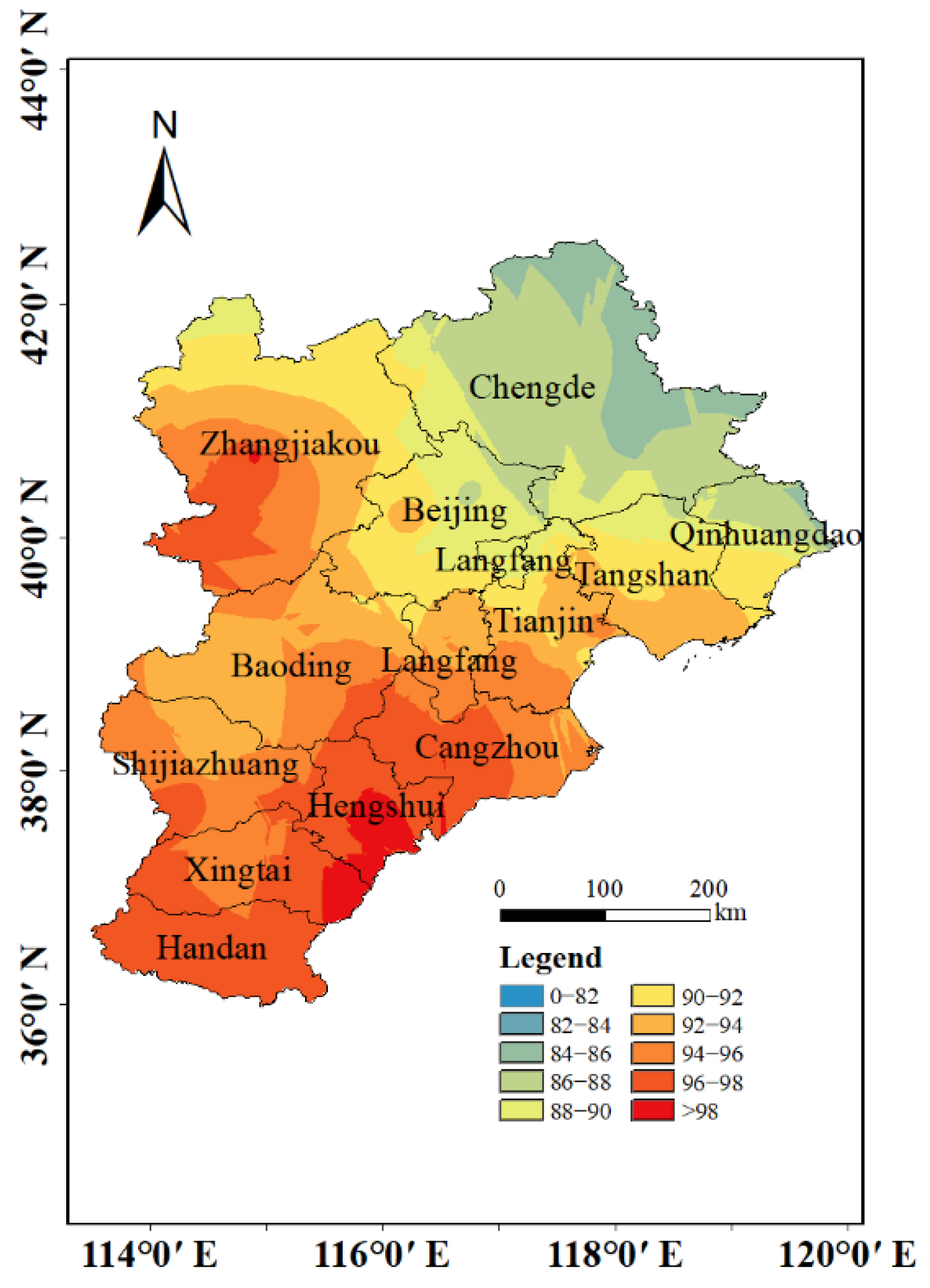
2.1. Study Domain
2.2. Data Collection and Processing
2.2.1. Air Pollutant Datasets
2.2.2. Meteorological Data
2.2.3. MERRA-2 Reanalysis Data
2.3. GWR Model Building
2.4. Cross-Validation
3. Result
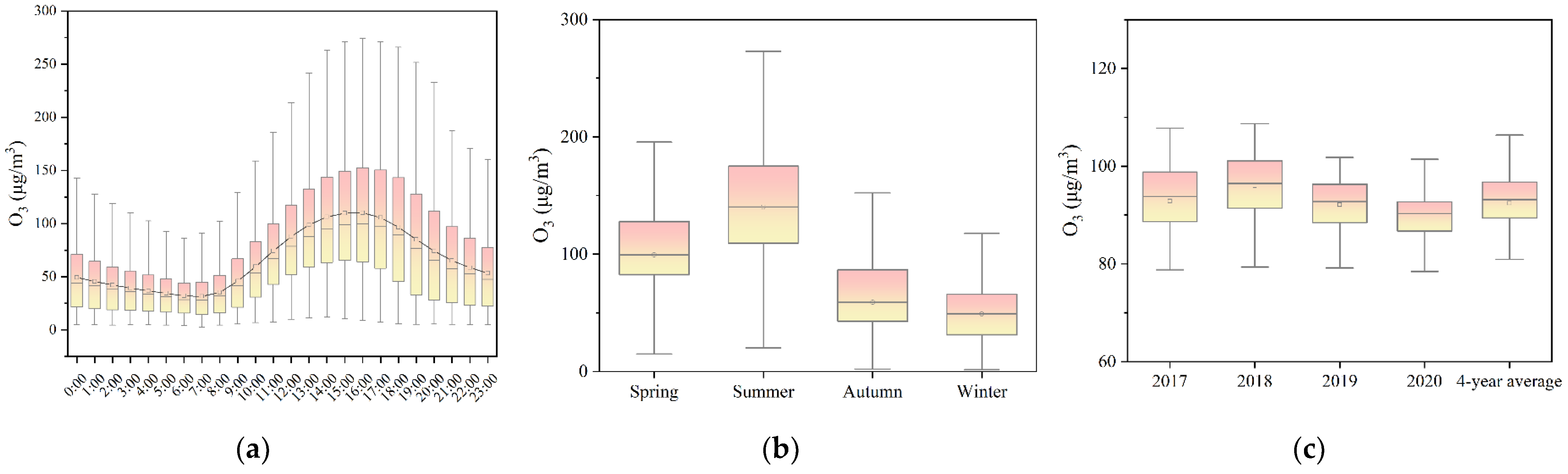
3.1. Exploratory Data Analysis
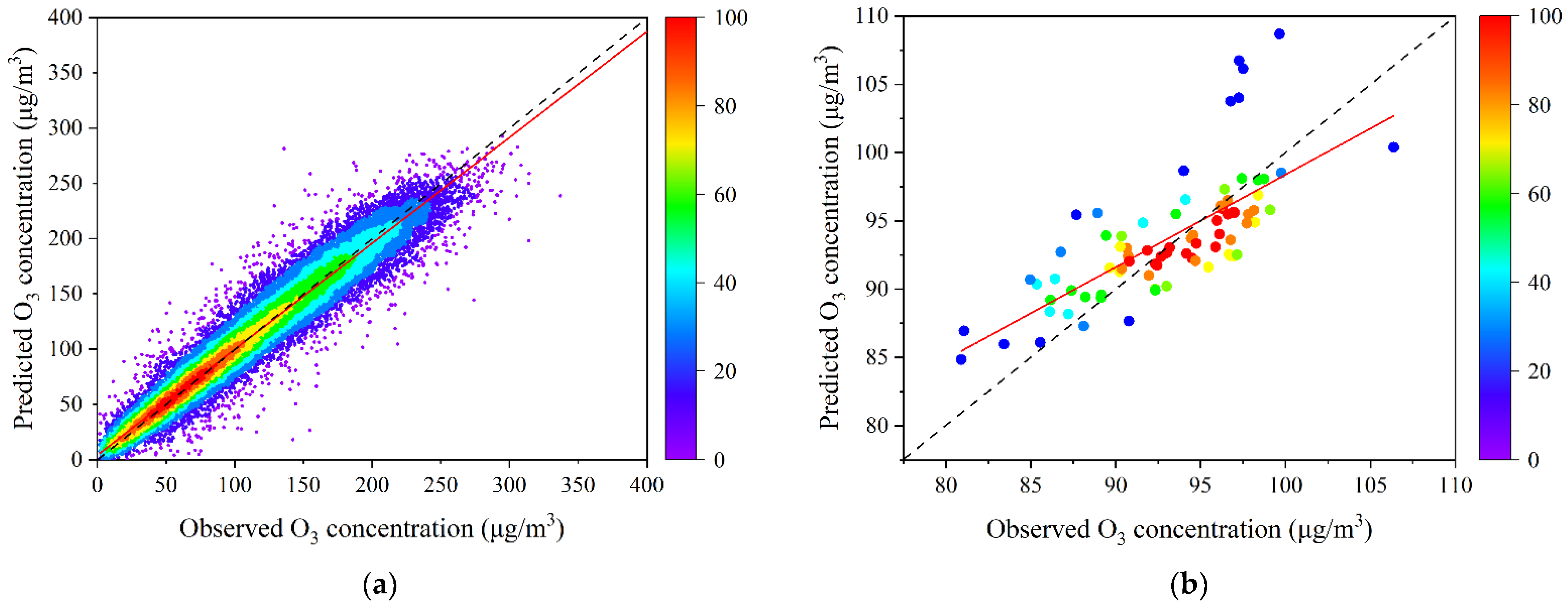
3.2. Model Fitting and Cross Validation
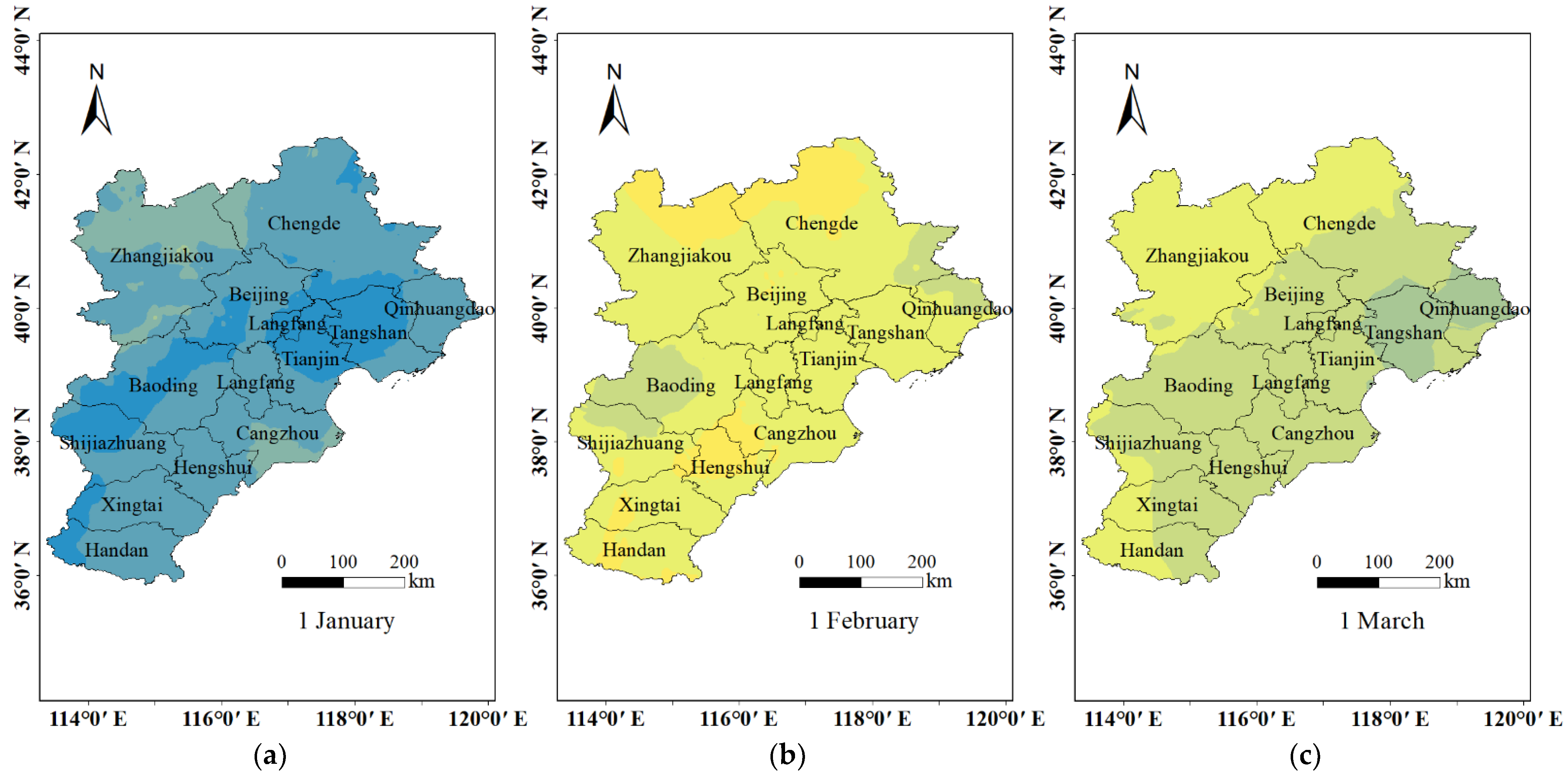
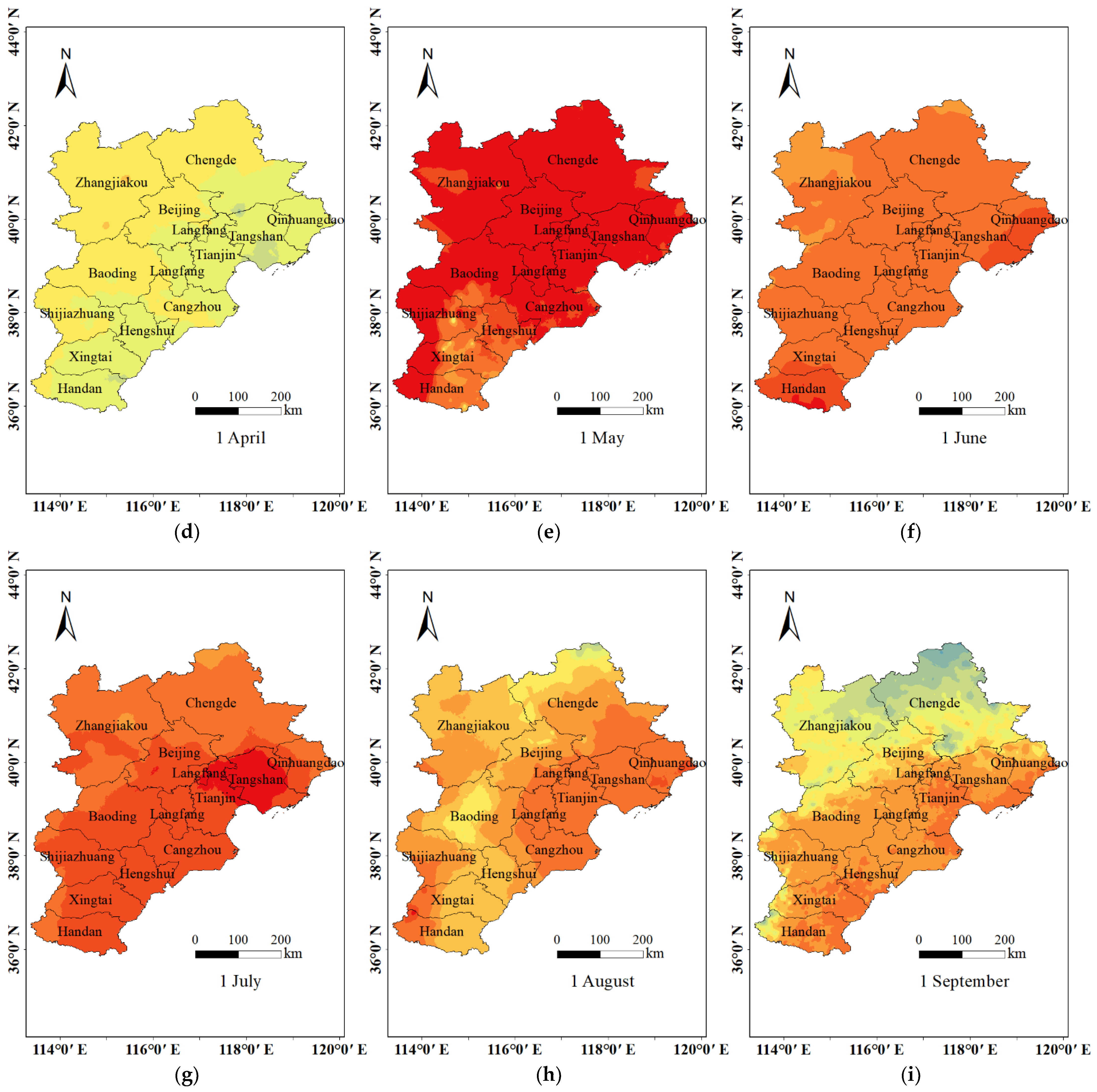
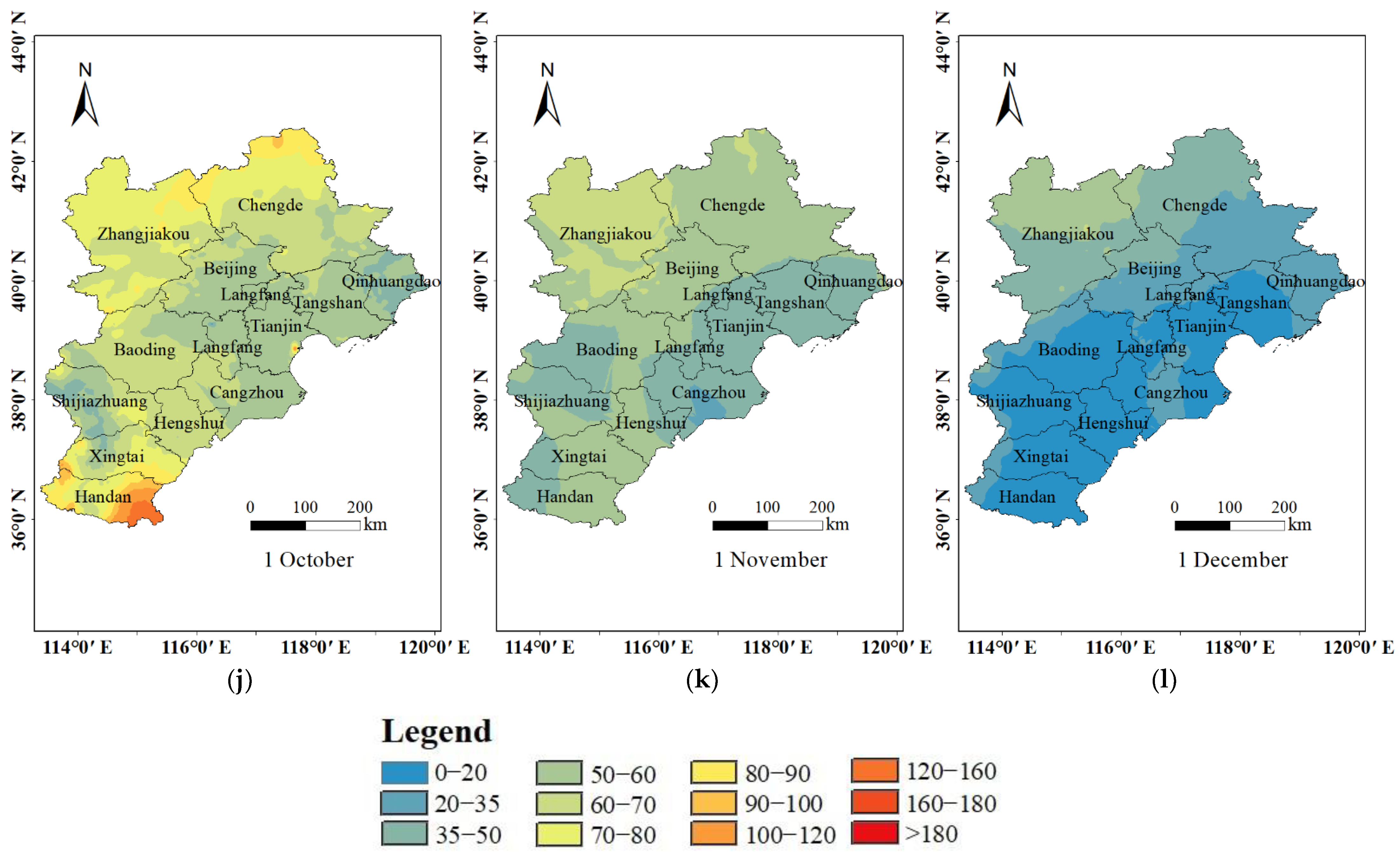
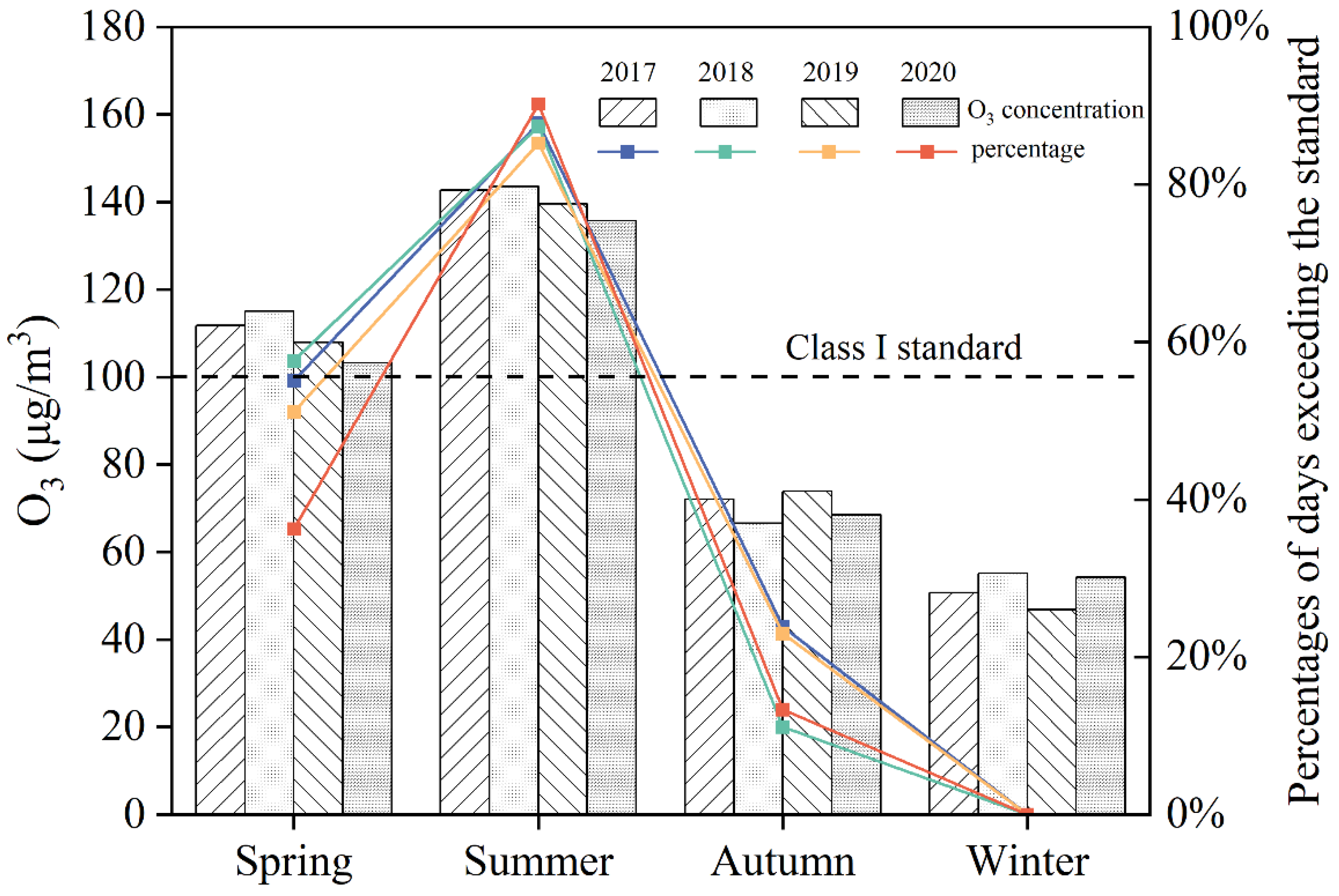
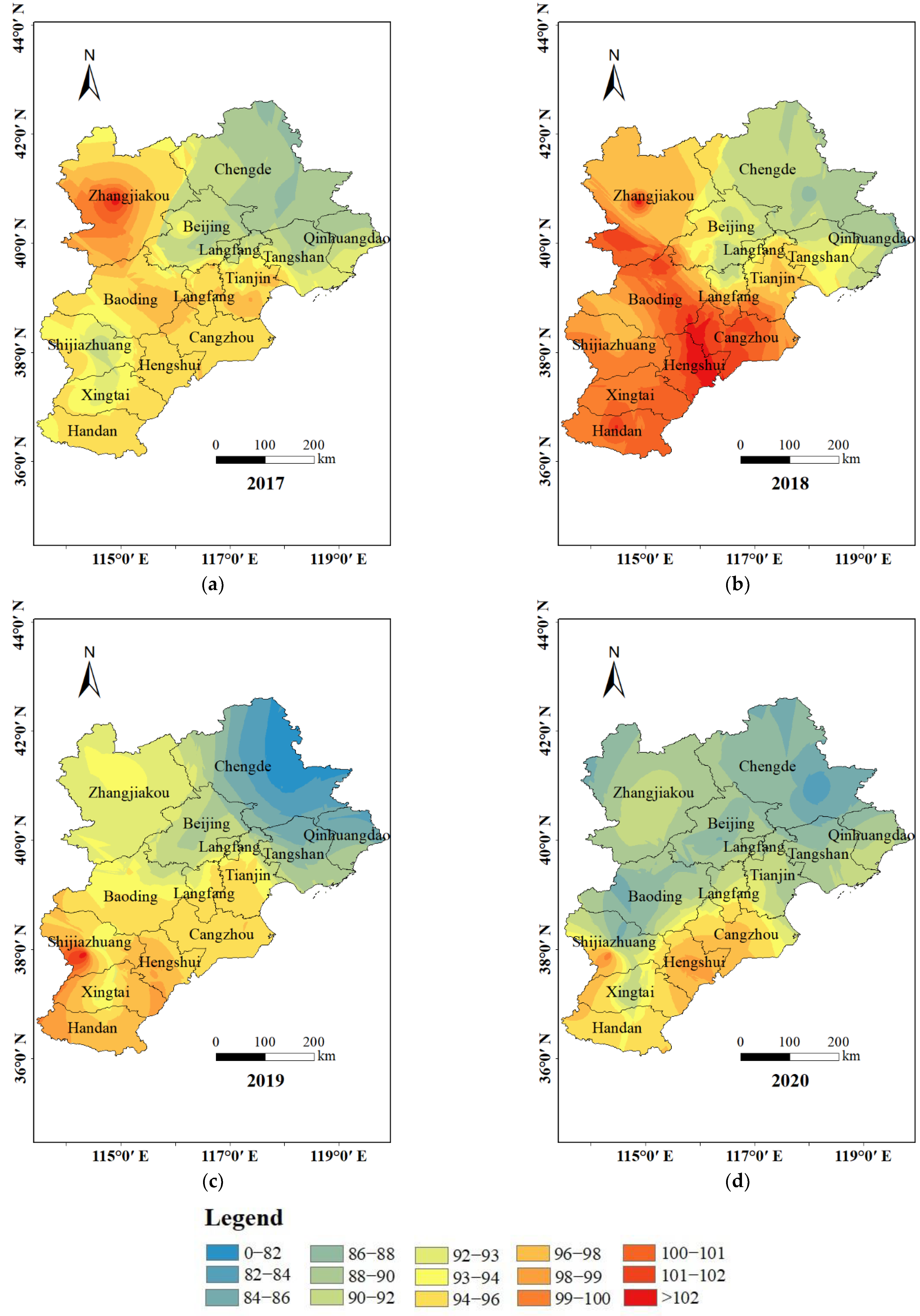
3.3. Spatio-Temporal Distribution of O3 Concentration
4. Discussion
5. Conclusions
Author Contributions
Funding
Institutional Review Board Statement
Informed Consent Statement
Data Availability Statement
Acknowledgments
Conflicts of Interest
References
- Wang, T.; Xue, L.K.; Brimblecombe, P.; Lam, Y.F.; Li, L.; Zhang, L. Ozone pollution in China: A review of concentrations, meteorological influences, chemical precursors, and effects. Sci. Total Environ. 2017, 575, 1582–1596. [Google Scholar] [CrossRef] [PubMed]
- Lefohn, A.S.; Malley, C.S.; Simon, H.; Wells, B.; Xu, X.B.; Zhang, L.; Wang, T. Responses of human health and vegetation exposure metrics to changes in ozone concentration distributions in the European Union, United States, and China. Atmos. Environ. 2017, 152, 123–145. [Google Scholar] [CrossRef] [Green Version]
- Lefohn, A.S.; Malley, C.S.; Smith, L.; Wells, B.; Hazucha, M.; Simon, H.; Naik, V.; Mills, G.; Schultz, M.G.; Paoletti, E.; et al. Tropospheric ozone assessment report: Global ozone metrics for climate change, human health, and crop/ecosystem research. Elem. Sci. Anthr. 2018, 6, 27. [Google Scholar] [CrossRef] [PubMed] [Green Version]
- Nuvolone, D.; Petri, D.; Voller, F. The effects of ozone on human health. Environ. Sci. Pollut. Res. 2018, 25, 8074–8088. [Google Scholar] [CrossRef]
- Zhang, J.F.; Wei, Y.J.; Fang, Z.F. Ozone Pollution: A Major Health Hazard Worldwide. Front. Immunol. 2019, 10, 2518. [Google Scholar] [CrossRef] [Green Version]
- Liu, H.; Liu, S.; Xue, B.R.; Lv, Z.F.; Meng, Z.H.; Yang, X.F.; Xue, T.; Yu, Q.; He, K.B. Ground-level ozone pollution and its health impacts in China. Atmos. Environ. 2018, 173, 223–230. [Google Scholar] [CrossRef]
- Sun, Q.; Wang, W.; Chen, C.; Ban, J.; Xu, D.; Zhu, P.; He, M.Z.; Li, T. Acute effect of multiple ozone metrics on mortality by season in 34 Chinese counties in 2013–2015. J. Intern. Med. 2018, 283, 481–488. [Google Scholar] [CrossRef]
- Liang, S.; Li, X.L.; Teng, Y.; Fu, H.C.; Chen, L.; Mao, J.; Zhang, H.; Gao, S.; Sun, Y.L.; Ma, Z.X.; et al. Estimation of health and economic benefits based on ozone exposure level with high spatial-temporal resolution by fusing satellite and station observations. Environ. Pollut. 2019, 255, 113267. [Google Scholar] [CrossRef]
- Guan, Y.; Xiao, Y.; Wang, Y.M.; Zhang, N.N.; Chu, C.J. Assessing the health impacts attributable to PM2.5 and ozone pollution in 338 Chinese cities from 2015 to 2020. Environ. Pollut. 2021, 287, 117623. [Google Scholar] [CrossRef]
- Zheng, D.Y.; Huang, X.J.; Guo, Y.H. Spatiotemporal variation of ozone pollution and health effects in China. Environ. Sci. Pollut. Res. 2022, 29, 57808–57822. [Google Scholar] [CrossRef]
- Bell, M.L.; Peng, R.D.; Dominici, F. The exposure-response curve for ozone and risk of mortality and the adequacy of current ozone regulations. Environ. Health Perspect. 2006, 114, 532–536. [Google Scholar] [CrossRef] [Green Version]
- Turner, M.C.; Jerrett, M.; Pope, C.A.; Krewski, D.; Gapstur, S.M.; Diver, W.R.; Beckerman, B.S.; Marshall, J.D.; Su, J.; Crouse, D.L.; et al. Long-Term Ozone Exposure and Mortality in a Large Prospective Study. Am. J. Respir. Crit. Care Med. 2016, 193, 1134–1142. [Google Scholar] [CrossRef] [Green Version]
- Zhang, X.X.; Cheng, C.X.; Zhao, H. A Health Impact and Economic Loss Assessment of O3 and PM2.5 Exposure in China from 2015 to 2020. Geohealth 2022, 6, e2021GH000531. [Google Scholar] [CrossRef]
- Ministry of Ecology and Environment of the People’s Republic of China. Bulletin of the State of the Environment in China for Year 2017. Available online: https://www.mee.gov.cn/hjzl/sthjzk/zghjzkgb/201805/P020180531534645032372.pdf (accessed on 23 September 2022).
- Ministry of Ecology and Environment of the People’s Republic of China. Bulletin of the State of the Environment in China for Year 2018. Available online: https://www.mee.gov.cn/hjzl/sthjzk/zghjzkgb/201905/P020190619587632630618.pdf (accessed on 23 September 2022).
- Ministry of Ecology and Environment of the People’s Republic of China. Bulletin of the State of the Environment in China for Year 2019. Available online: https://www.mee.gov.cn/hjzl/sthjzk/zghjzkgb/202006/P020200602509464172096.pdf (accessed on 23 September 2022).
- Ministry of Ecology and Environment of the People’s Republic of China. Bulletin of the State of the Environment in China for Year 2020. Available online: https://www.mee.gov.cn/hjzl/sthjzk/zghjzkgb/202105/P020210526572756184785.pdf (accessed on 23 September 2022).
- Chen, L.; Liang, S.; Li, X.L.; Mao, J.; Gao, S.; Zhang, H.; Sun, Y.L.; Vedal, S.; Bai, Z.P.; Ma, Z.X.; et al. A hybrid approach to estimating long-term and short-term exposure levels of ozone at the national scale in China using land use regression and Bayesian maximum entropy. Sci. Total Environ. 2021, 752, 141780. [Google Scholar] [CrossRef]
- Wang, W.N.; Cheng, T.H.; Gu, X.F.; Chen, H.; Guo, H.; Wang, Y.; Bao, F.W.; Shi, S.Y.; Xu, B.R.; Zuo, X.; et al. Assessing Spatial and Temporal Patterns of Observed Ground-level Ozone in China. Sci. Rep. 2017, 7, 3651. [Google Scholar] [CrossRef]
- Zhao, S.H.; Yang, X.Y.; Li, Z.Q.; Wang, Z.T.; Zhang, Y.H.; Wang, Y.; Zhou, C.Y.; Ma, P.F. Advances of ozone satellite remote sensing in 60 years. Natl. Remote Sens. Bull. 2022, 26, 817–833. [Google Scholar]
- Chianese, E.; Galletti, A.; Giunta, G.; Landi, T.C.; Marcellino, L.; Montella, R.; Riccio, A. Spatiotemporally resolved ambient particulate matter concentration by fusing observational data and ensemble chemical transport model simulations. Ecol. Model. 2018, 385, 173–181. [Google Scholar] [CrossRef]
- Akita, Y.; Baldasano, J.M.; Beelen, R.; Cirach, M.; de Hoogh, K.; Hoek, G.; Nieuwenhuijsen, M.; Serre, M.L.; de Nazelle, A. Large Scale Air Pollution Estimation Method Combining Land Use Regression and Chemical Transport Modeling in a Geostatistical Framework. Environ. Sci. Technol. 2014, 48, 4452–4459. [Google Scholar] [CrossRef] [Green Version]
- Hu, L.M.; Li, Y.X.; Shi, N.F.; Su, J. Spatio-temporal Change Characteristics of Ozone Concentration in Beijing-Tianjin-Hebei Region. Environ. Sci. Technol. 2019, 42, 1–7. [Google Scholar]
- Zhang, H.; Zhan, Y.; Li, J.Y.; Chao, C.Y.; Liu, Q.F.; Wang, C.Y.; Jia, S.Q.; Ma, L.; Biswas, P. Using Kriging incorporated with wind direction to investigate ground-level PM2.5 concentration. Sci. Total Environ. 2021, 751, 141813. [Google Scholar] [CrossRef]
- Li, J.; Heap, A.D. Spatial interpolation methods applied in the environmental sciences: A review. Environ. Model. Softw. 2014, 53, 173–189. [Google Scholar] [CrossRef]
- Couzo, E.; Olatosi, A.; Jeffries, H.E.; Vizuete, W. Assessment of a regulatory model’s performance relative to large spatial heterogeneity in observed ozone in Houston, Texas. J. Air Waste Manag. Assoc. 2012, 62, 696–706. [Google Scholar] [CrossRef] [PubMed]
- Narayan, T.; Bhattacharya, T.; Chakraborty, S.; Konar, S. Application of Multiple Linear Regression and Geographically Weighted Regression Model for Prediction of PM2.5. Proc. Natl. Acad. Sci. India Sect. A Phys. Sci. 2022, 92, 217–229. [Google Scholar] [CrossRef]
- Brunsdon, C.; Fotheringham, A.S.; Charlton, M.E. Geographically weighted regression: A method for exploring spatial nonstationarity. Geogr. Anal. 1996, 28, 281–298. [Google Scholar] [CrossRef]
- Stowell, J.D.; Bi, J.Z.; Al-Hamdan, M.Z.; Lee, H.J.; Lee, S.M.; Freedman, F.; Kinney, P.L.; Liu, Y. Estimating PM2.5 in Southern California using satellite data: Factors that affect model performance. Environ. Res. Lett. 2020, 15, 094004. [Google Scholar] [CrossRef]
- Shen, Y.; de Hoogh, K.; Schmitz, O.; Clinton, N.; Tuxen-Bettman, K.; Brandt, J.; Christensen, J.H.; Frohn, L.M.; Geels, C.; Karssenberg, D.; et al. Europe-wide air pollution modeling from 2000 to 2019 using geographically weighted regression. Environ. Int. 2022, 168, 107485. [Google Scholar] [CrossRef]
- Ma, R.M.; Ban, J.; Wang, Q.; Zhang, Y.Y.; Yang, Y.; He, M.K.Z.; Li, S.S.; Shi, W.J.; Li, T.T. Random forest model based fine scale spatiotemporal O3 trends in the Beijing-Tianjin-Hebei region in China, 2010 to 2017. Environ. Pollut. 2021, 276, 116635. [Google Scholar] [CrossRef]
- Lyu, Y.; Ju, Q.R.; Lv, F.M.; Feng, J.L.; Pang, X.B.; Li, X. Spatiotemporal variations of air pollutants and ozone prediction using machine learning algorithms in the Beijing-Tianjin-Hebei region from 2014 to 2021. Environ. Pollut. 2022, 306, 119420. [Google Scholar] [CrossRef]
- Hu, X.M.; Zhang, J.; Xue, W.H.; Zhou, L.H.; Che, Y.F.; Han, T. Estimation of the Near-Surface Ozone Concentration with Full Spatiotemporal Coverage across the Beijing-Tianjin-Hebei Region Based on Extreme Gradient Boosting Combined with a WRF-Chem Model. Atmosphere 2022, 13, 632. [Google Scholar] [CrossRef]
- Wei, J.; Li, Z.Q.; Li, K.; Dickerson, R.R.; Pinker, R.T.; Wang, J.; Liu, X.; Sun, L.; Xue, W.H.; Cribb, M. Full-coverage mapping and spatiotemporal variations of ground-level ozone (O3) pollution from 2013 to 2020 across China. Remote Sens. Environ. 2022, 270, 112775. [Google Scholar] [CrossRef]
- Xue, W.H.; Zhang, J.; Hu, X.M.; Yang, Z.; Wei, J. Hourly Seamless Surface O3 Estimates by Integrating the Chemical Transport and Machine Learning Models in the Beijing-Tianjin-Hebei Region. Int. J. Environ. Res. Public Health 2022, 19, 8511. [Google Scholar] [CrossRef] [PubMed]
- Masri, S.; Hou, H.Y.; Dang, A.; Yao, T.; Zhang, L.W.; Wang, T.; Qin, Z.; Wu, S.Y.; Hang, B.; Chen, J.C.; et al. Development of spatiotemporal models to predict ambient ozone and NOx concentrations in Tianjin, China. Atmos. Environ. 2019, 213, 37–46. [Google Scholar] [CrossRef]
- Dong, Y.M.; Li, J.; Guo, J.P.; Jiang, Z.J.; Chu, Y.Q.; Chang, L.; Yang, Y.; Liao, H. The impact of synoptic patterns on summertime ozone pollution in the North China Plain. Sci. Total Environ. 2020, 735, 139559. [Google Scholar] [CrossRef] [PubMed]
- Wang, M.; Zheng, Y.F.; Liu, Y.J.; Li, Q.P.; Ding, Y.H. Characteristics of ozone and its relationship with meteorological factors in Beijing-Tianjin-Hebei Region. China Environ. Sci. 2019, 39, 2689–2698. [Google Scholar]
- Yao, Q.; Fan, W.Y.; Huang, H.; Sun, M.L.; Liu, A.X. Variation of surface O3 concentration and its influencing factors in summer in Tianjin. Ecol. Environ. Sci. 2009, 18, 12–16. [Google Scholar]
- Wang, Y.L.; Xue, W.B.; Lei, Y.; Wu, W.L. Model-derived source apportionment and regional transport matrix study of ozone in Jingjinji. China Environ. Sci. 2017, 37, 3684–3691. [Google Scholar]
- Rahman, M.M.; Shuo, W.; Zhao, W.X.; Xu, X.Z.; Zhang, W.J.; Arshad, A. Investigating the Relationship between Air Pollutants and Meteorological Parameters Using Satellite Data over Bangladesh. Remote Sens. 2022, 14, 2757. [Google Scholar] [CrossRef]
- Mao, J.; Wang, L.L.; Lu, C.H.; Liu, J.D.; Li, M.G.; Tang, G.Q.; Ji, D.S.; Zhang, N.; Wang, Y.S. Meteorological mechanism for a large-scale persistent severe ozone pollution event over eastern China in 2017. J. Environ. Sci. 2020, 92, 187–199. [Google Scholar] [CrossRef]
- Li, H.; Wang, S.L.; Zhang, W.J.; Wang, H.; Wang, H.; Wang, S.B.; Li, H.S. Characteristics and Influencing Factors of Urban Air Quality in Beijing-Tianjin Hebei and Its Surrounding Areas (‘2 + 26’ Cities). Res. Environ. Sci. 2021, 34, 172–184. [Google Scholar]
- Adame, J.A.; Lozano, A.; Bolivar, J.P.; De la Morena, B.A.; Contreras, J.; Godoy, F. Behavior, distribution and variability of surface ozone at an arid region in the south of Iberian Peninsula (Seville, Spain). Chemosphere 2008, 70, 841–849. [Google Scholar] [CrossRef]
- Yao, Q.; Ma, Z.Q.; Hao, T.Y.; Fan, W.Y.; Yang, X.; Tang, Y.X.; Cai, Z.Y.; Han, S.Q. Temporal and spatial distribution characteristics and background concentration estimation of ozone in Beijing-Tianjin-Hebei region. China Environ. Sci. 2021, 41, 4999–5008. [Google Scholar]
- Qi, J.; Zheng, B.; Li, M.; Yu, F.; Chen, C.C.; Liu, F.; Zhou, X.F.; Yuan, J.; Zhang, Q.; He, K.B. A high-resolution air pollutants emission inventory in 2013 for the Beijing-Tianjin-Hebei region, China. Atmos. Environ. 2017, 170, 156–168. [Google Scholar] [CrossRef]
- Beijing Bureau of Statistics of China. Beijing Statistical Year Book 2021; China Statistics Press: Beijing, China, 2021. Available online: http://nj.tjj.beijing.gov.cn/nj/main/2021-tjnj/zk/indexch.htm (accessed on 23 September 2022).
- Hebei Bureau of Statistics of China. Hebei Statistical Year Book 2021; China Statistics Press: Hebei, China, 2021. Available online: http://tjj.hebei.gov.cn/hetj/tjnj/2021/zk/indexch.htm (accessed on 23 September 2022).
- Tianjin Bureau of Statistics of China. Tianjin Statistical Year Book 2021; China Statistics Press: Tianjin, China, 2021. Available online: http://stats.tj.gov.cn/nianjian/2021nj/zk/indexch.htm (accessed on 23 September 2022).


| Year | Point | Valid Value | Min (μg/m3) | Max (μg/m3) | Mean (μg/m3) | Median (μg/m3) |
|---|---|---|---|---|---|---|
| 2017 | 83 | 28,175 | 1.46 | 476.63 | 93.64 | 83.38 |
| 2018 | 80 | 27,927 | 2.50 | 314.33 | 95.98 | 84.90 |
| 2019 | 80 | 27,820 | 1.50 | 319.5 | 92.25 | 82.65 |
| 2020 | 82 | 28,832 | 3.08 | 366.58 | 90.49 | 81.63 |
| O3 (μg/m3) | PM2.5 (μg/m3) | PM10 (μg/m3) | CO (μg/m3) | NO2 (μg/m3) | SO2 (μg/m3) | Precipitation (mm) | |
| Mean | 93.07 | 53.01 | 95.63 | 1.02 | 40.43 | 15.66 | 1.30 |
| Min | 1.46 | 2.62 | 5.19 | 0.10 | 1.54 | 1.00 | 0 |
| Max | 476.63 | 644.14 | 1767.46 | 10.00 | 188.29 | 261.45 | 158.25 |
| Standard deviation | 52.23 | 44.68 | 68.73 | 0.70 | 21.13 | 14.78 | 6.03 |
| Pressure (hPa) | Relative Humidity (%) | Temperature (°C) | Wind Speed (m/s) | AOD | PBLH (m) | TI (°C/100 m) | |
| Mean | 1004.24 | 55.76 | 13.76 | 1.66 | 0.47 | 815.48 | 0.45 |
| Min | 869.63 | 7.24 | −21.12 | 0.05 | 0.02 | 63.90 | 0 |
| Max | 1043.97 | 99.56 | 34.84 | 7.35 | 4.37 | 3651.20 | 4.95 |
| Standard deviation | 26.21 | 19.25 | 11.36 | 0.77 | 0.37 | 464.45 | 0.60 |
| Variables | β | p | VIF |
|---|---|---|---|
| Intercept | 93.036 | <0.001 | NA |
| Precipitation | −1.385 | 0.002 | 1.572 |
| Temperature | 4.235 | <0.001 | 1.812 |
| NO2 | −3.951 | <0.001 | 2.574 |
| Wind speed | 1.304 | <0.001 | 1.043 |
| SO2 | 0.986 | 0.041 | 1.993 |
Publisher’s Note: MDPI stays neutral with regard to jurisdictional claims in published maps and institutional affiliations. |
© 2022 by the authors. Licensee MDPI, Basel, Switzerland. This article is an open access article distributed under the terms and conditions of the Creative Commons Attribution (CC BY) license (https://creativecommons.org/licenses/by/4.0/).
Share and Cite
Qiao, Z.; Liu, Y.; Cui, C.; Shan, M.; Tu, Y.; Liu, Y.; Xu, S.; Mi, K.; Chen, L.; Ma, Z.; et al. Estimation of Short-Term and Long-Term Ozone Exposure Levels in Beijing–Tianjin–Hebei Region Based on Geographically Weighted Regression Model. Atmosphere 2022, 13, 1706. https://doi.org/10.3390/atmos13101706
Qiao Z, Liu Y, Cui C, Shan M, Tu Y, Liu Y, Xu S, Mi K, Chen L, Ma Z, et al. Estimation of Short-Term and Long-Term Ozone Exposure Levels in Beijing–Tianjin–Hebei Region Based on Geographically Weighted Regression Model. Atmosphere. 2022; 13(10):1706. https://doi.org/10.3390/atmos13101706
Chicago/Turabian StyleQiao, Zequn, Yusi Liu, Chen Cui, Mei Shan, Yan Tu, Yaxin Liu, Shiwen Xu, Ke Mi, Li Chen, Zhenxing Ma, and et al. 2022. "Estimation of Short-Term and Long-Term Ozone Exposure Levels in Beijing–Tianjin–Hebei Region Based on Geographically Weighted Regression Model" Atmosphere 13, no. 10: 1706. https://doi.org/10.3390/atmos13101706