Assessing Indoor Environmental Quality in a Crowded Low-Quality Built Environment: A Case Study

Abstract

Home heating, cooling and ventilation are a major concern for those living in low-quality built environments, particularly those with high occupancy rates (crowded houses). In New Zealand, both owner-occupiers and tenants can experience problems associated with poor Indoor Environmental Quality (IEQ), such as poor thermal comfort and dampness, when Heating Ventilation and Air-Conditioning (HVAC) systems are not installed, improperly installed or too expensive to run. Occupants of poorer households are the most affected by high installation or running costs of HVAC systems, and are also more likely to live in households with a higher level of crowding. Poor IEQ in housing is associated with adverse health outcomes, particularly respiratory illness. This paper outlines the IEQ problems experienced by households living in an area of New Zealand with higher levels deprivation and shows how an HVAC system could be employed to remedy poor IEQ. This report presents a case study of a house with poor IEQ that was selected from a survey conducted across 24 homes in the Manukau, Auckland region of New Zealand. The IEQ results are presented for this house, which performs poorly in terms of relative humidity, temperature and thermal comfort. This house is then analysed using the computational fluid dynamics (CFD) approach in ANSYS CFX 2021R1 based on the American Society of Heating, Refrigeration and Airconditioning Engineers (ASHRAE) standard 55-2017 and a model of temperature and air flow is created in the software, which can identify ways to improve these parameters in the house. These results are compared with the New Zealand Healthy Homes Standards 2019. The simulation showed the system was capable of lifting the indoor temperature to above $21 ℃$, eliminating cold spots and improving thermal comfort, and reduced relative humidity to below 50%.

1. Introduction

The price of housing has been steadily increasing in New Zealand, a trajectory sometimes punctuated by steep increases. This has translated to higher mortgage repayments and higher rental costs for tenants. Across the last 15 years, the average weekly rental has risen by 84.3%, whilst average household disposable income only increased by 67.6% [1]. Low income households frequently must respond to rising housing costs by increasing the occupancy rate of the house: taking in more paying tenants, moving to a smaller house with fewer bedrooms, or moving in with family to share the housing cost. This leads to crowding where the number of occupants of a house exceeds the recommended number according to occupancy standards.

In New Zealand, the indigenous people (Māori) and those with Pacific Island heritage (Pacifica), are among those most severely impacted by crowding [2]. In the Auckland region, the Manukau area is one of the higher deprivation areas, as well as having a higher percentage of Māori and Pacific peoples: 17.1% and 25.3%, respectively [3].

Crowding enables airborne respiratory diseases to spread more efficiently due to the greater number and closer proximity of occupants. This effect intensifies when families must sleep in one room to save on heating costs. The effect is most pronounced for infants and young children, leading to a greater incidence of respiratory infections and hospital admissions for this group [4,5].

In addition, New Zealand is a country with high relative humidity (dampness), and a relatively old housing stock with a high proportion constructed of wood [6]. Centralised HVAC systems are rare, with after-market solutions quite common, such as the installation of single-room split unit heating and cooling systems (heat pumps) and positive air pressure ventilation systems. These devices and systems are costly to install; however, heat pumps are increasingly being installed by landlords, in order to comply with the New Zealand Healthy Homes 2019 Regulations [7]. Other forms of space heating involve less expensive upfront costs, but higher running costs, meaning that such devices remain switched off in order to save power. Therefore, many homes exhibit poor indoor environmental quality (IEQ): low thermal comfort (cold), high relative humidity (damp), airborne pathogens, and other indoor air quality (IAQ) problems, including harmful particulate matters caused by mould spores. These homes increase the risk to occupants of respiratory conditions and preventable illnesses [7].

Poor thermal comfort is a particular problem in New Zealand houses. In their 2021 study of 2000 children in New Zealand, Morton et al. (2021) found that 50% of children routinely slept in bedrooms that were too cold [8]. Approximately 1000 of the children in their surveys experienced ambient temperatures that fell below 19$℃$ overnight, with some children’s bedrooms registering temperatures below 4$℃$ overnight [8].

Engineering studies [9,10,11,12,13,14,15] enable numerical and computational analysis of thermal comfort to propose potential solutions to address the issues described above. In particular the computational fluid dynamics (CFD) method can inform of thermal comfort issues, and can be deployed in a number of software packages. Pérez et al. [9] used CFD in Star (Computational Continuum Mechanics (CCM+)) to investigate the effect of fresh inlet air on IEQ (including thermal comfort) in a multipurpose room. In Wahhad et al. 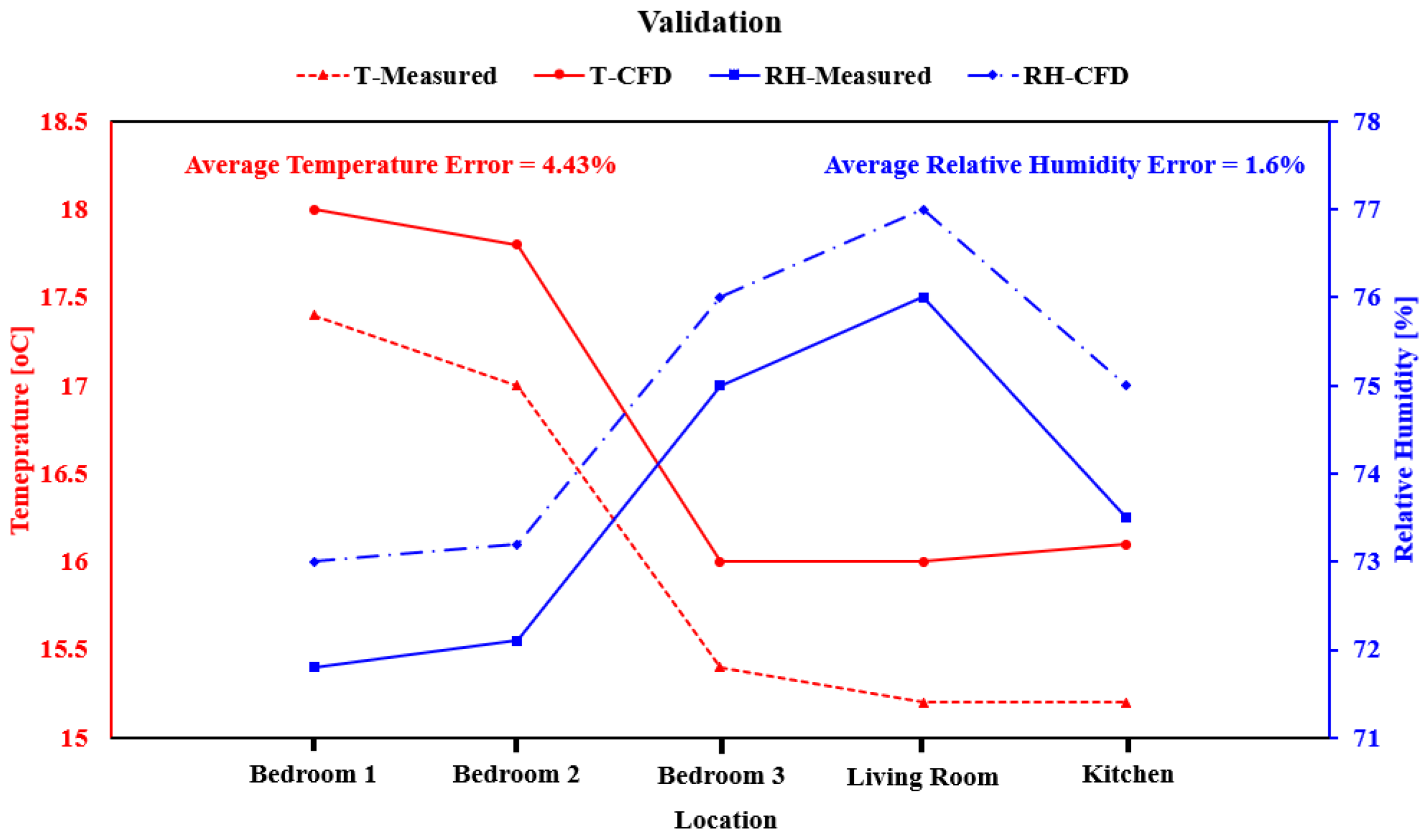[11], CFD analysis was conducted in ANSYS-Fluent to examine the disparity between outdoor and indoor temperatures, as well as the distribution of temperatures within the indoor space. The results of their CFD analysis align with the experimental data, having an 8.23% maximum accuracy error, using k-ε and Reynolds stress models. Raczkowski et al. [12] used the standard k–ε model in Autodesk Inventor to study the temperature profiles when mixing indoor with outdoor air during heating, in terms of the Predicted Mean Vote (PMV) and Predicted Percentage Dissatisfied (PPD) thermal comfort parameters. They found that the PMV and PPD confirmed their measured data, reflecting that CFD can be used to accurately predict performance of thermal parameters. Al-Rawi et al. [13] conducted CFD analysis in ANSYS Fluent to investigate the behavior of air velocity contours in a residential home office when one occupant coughs. They also examined thermal comfort parameters including temperature, PMV and PPD at different times, and validated the CFD results with data taken using the Testo 400 IAQ and comfort kit (Testo SE & Co. KGaA, Lenzkirch, Germany). These data closely agreed with the results of the CFD model, further illustrating the usefulness of CFD for predicting these thermal comfort parameters.

In this paper we present a survey of the case study house, including house dimensions, occupancy, readings of air temperature, air velocity, relative humidity, moisture content and thermal imaging for the living areas of the house. Then, a model of the house was designed and analysed in terms of air temperature and air velocity. We then outline a potential Heating, Ventilation and Air- Conditioning (HVAC) system, a ducted heat pump system, on a simulated model of the house, assessing the system’s potential impact on this case-study house, in terms of temperature, air velocities, relative humidity and thermal comfort parameters, using ANSYS -CFX 2021 R1 (Ansys, Inc., Canonsburg, PA, USA). This study reflects analysis of IEQ using CFD methods and a proposed solution for a house in realistic sub-optimal living conditions in New Zealand where houses are frequently too cold, have high relative humidity and may have high occupancy in some or all rooms. To the best of our knowledge, this is the first such study of a home with poor IEQ and high occupancy for which this analysis has been performed.

2. Materials and Methods

This study selects a single house from a collection of 24 home surveys that were conducted for the winter months (June to August in New Zealand), in the Manukau area of Auckland, New Zealand. The case study was selected because the house exhibited poor IEQ and, due to the distribution of occupants in each room, one room in the house would be described as crowded, according to the Canadian National Occupancy Standards [16]. Ethical approval (E15/FET/14) was obtained for this survey, and collection of data for the house was done in accordance with ethical protocols, with data stored in accordance with the New Zealand Privacy Act.

This house contained four adults and one infant aged nine months old. Due to high electricity bills, the occupants revealed they were not running the heaters in the house.

Table 1. Instrument used for measuring temperature and relative humidity.

Instrument	Parameters	Values
Thermometer/laser meter	Temperature	$\mathrm{Range}: -$10 to 50 °C,
		$\mathrm{Accuracy}: \pm$0.3 °C
Testo 410-2 NTC, Rotary Vane 20 m/s	Air Velocity (m/s2)	Max Air Velocity 20 m/s
		$\mathrm{Accuracy}: \pm$$2\% +$ 0.2 m/s
Forward Looking InfraRed (FLIR) Thermal Camera	Thermal Images	$\mathrm{Range}: -$$25 \mathrm{to} +$150 °C
		$\mathrm{Accuracy}: \pm$ 1.5 °C
PROTIMETER MMS2	Relative Humidity (%), Moisture level (%)	Range: 41 to 98% RH,
		$\mathrm{Accuracy}: \pm$2% RH at 20 °C

below presents the IEQ measures taken for the case study house, along with the specifications of the instrument used to collect each measure.

Table 2. Indoor Environmental Quality measurements for the case study house (excludes the bathroom, due to occupants’ request).

Location	Average Moisture Content (%)	Relative Humidity (%)	Temperature $(℃)$	Number of Occupants
Bedroom 1	125.75	71.8	17.4	1
Bedroom 2	123.25	72.1	17	3
Bedroom 3	126.25	75	15.4	1
Living Room	124	76	15.2	5
Kitchen	126.75	73.5	15.2	NA

presents the IEQ measures for the case study house and Figure 1 presents the thermal images for areas the house. The air velocity reading was zero for all rooms, therefore this is not included in the table. As shown in Table 2, the ambient temperature in all rooms was slightly cold, and below the minimum of 19.4$°\mathrm{C}$ recommended by the American Society of Heating, Refrigeration and Airconditioning Engineers (ASHRAE) [17].

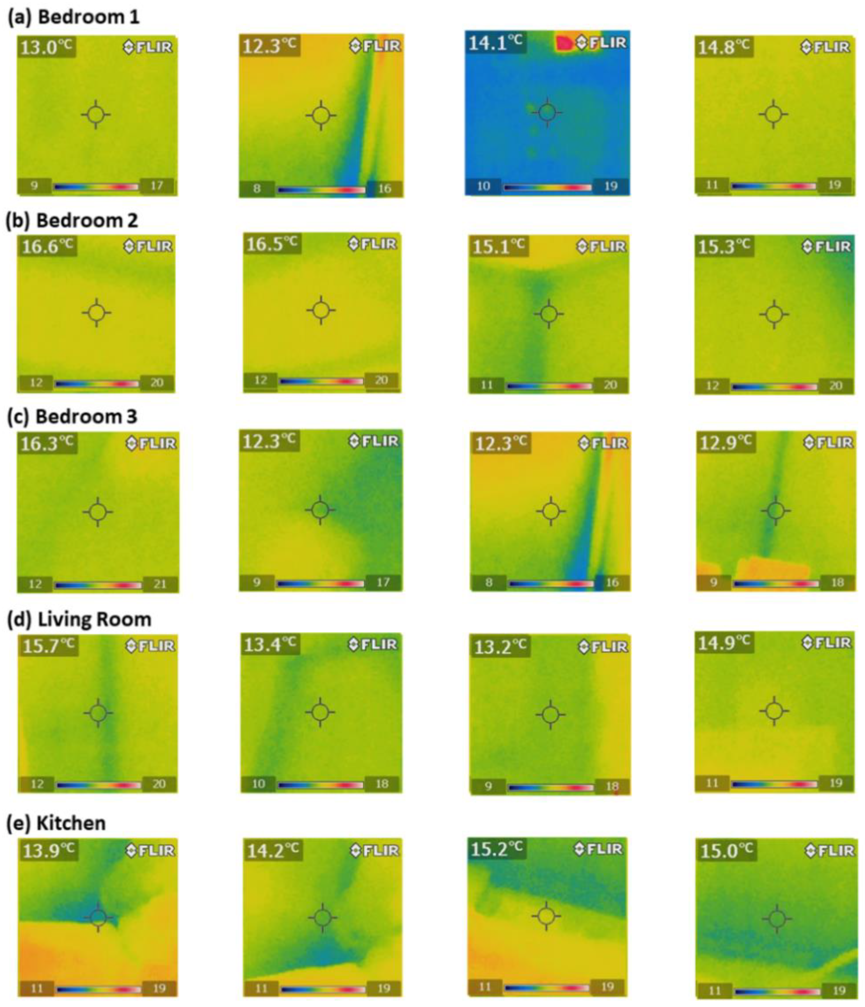
The thermal images, which were obtained as part of the home survey, provide richer information on temperature, as they show the high and low points of temperature in a given area of the room (e.g., at the corner). They help to explain why some rooms can feel colder than the measured temperature, where streams of cooler air enter the room through uninsulated portions of the wall or ceiling. The temperature measured at each area of the room shown in Figure 1 was, on average, lower than the ambient temperature in the room, and the scale (at the bottom of each panel) shows the coolest part of the area in bedrooms 1 and 3 reached as low as 8$°\mathrm{C}$.

The house did exhibit dampness, with the indoor relative humidity measure exceeding the relative humidity outside. As Table 2 illustrates, all measures for relative humidity exceeded 70%, with the average relative humidity for all rooms being 73.68%; this is higher than the 30–50% recommended level for relative humidity [18]. Therefore, the measurement obtained from this house shows the potential for increased mould and fungi growth on the building materials [19].

The thermal images were taken using the FLIR thermal imaging camera to determine the temperatures on those surfaces. Figure 1 shows the top corner surface images for the walls of each room in the house. As described above, the surface wall temperature in bedrooms 1 and 3 (Figure 1a,c) were colder compared to bedroom 2. As shown in Table 2, bedrooms 1 and 3 each had one occupant whilst bedroom 2 had two adults and one infant (see Figure 1b). In bedroom 1 the average surface temperatures for each wall ranged from 12.3$℃$ to 14.8$℃$, with the coldest surface area reading 8$℃$ and the warmest 19$℃$, while bedroom 3 had an average temperature range between 12.3$℃$ and 16.3$℃$, with the coldest surface area reading 8$℃$ and the warmest 21$℃$. Bedroom 2′s average temperature for each wall measured between 15.1$℃$ and 16.6$℃$ with a smaller range: the coldest surface area reading 11$℃$ and the warmest was 20$℃$. This greater warmth could be due to the number of occupants in the room. Figure 1d,e shows the surface temperature for the living room and kitchen. Respectively, these ranged from 13.2$℃$ to 15.7$℃$ and 13.9$℃$ to 15.2$℃$.

Non-invasive (pin-less) moisture meter readings were also taken for all four walls using the PROTIMETER MMS2, General Electric Company, Boston, MA, USA. Table 2 displays these readings. The Wood Moisture Equivalent (WME) value can be seen in Table 2. For this house, the WME values range from 110 to 131, which are in the dry range [20]. This indicated that the house did not have any water ingress issues or structural defects that affected weather-tightness of the building envelope.

3. Model Simulation

A model of the case-study house is simulated using ANSYS CFX Version 2021 R1 (Figure 2), to identify the potential to improve the ventilation, air flow and temperature via an HVAC system in the house. The house dimensions are 11 × 9 × 3 m. The proposed system modeled here would be achieved through a ducted heat pump system; the precise specifications of the heat pump and ducting are not included in this study. After constructing the CAD file using Design Modeler in the ANSYS workbench, we then set up the physical conditions.

3.1. Physical Model

The flow simulation model was constructed with internal steady turbulence flow and no-slip wall boundary conditions. The fluid concentration consisted of a 50:50 mix of fresh air and expired (exhaled) air, assuming an adiabatic wall. Flow simulation in ANSYS CFX solves the three equations below.

The continuity equation:

$$\frac{\partial \rho }{\partial t}+\nabla ·\left(\rho U\right)=0$$

(1)

The conservation of momentum equation:

$$\frac{\partial \left(\rho U\right)}{\partial t}+\nabla ·\left(\rho U\otimes U\right)=-\nabla p+\nabla ·\tau +\rho g+F$$

(2)

The energy equation:

$$\frac{\partial \left(\rho h_{tot}\right)}{\partial t}-\frac{\partial p}{\partial t}+\nabla ·\left(\rho U{h}_{tot}\right)=\nabla ·\left(U·\tau \right)+U·S_M+S_E$$

(3)

given:

$$\begin{gathered} \tau =\mu \left(\nabla U+{\left(\nabla U\right)}^T-\frac{2}{3}\delta \nabla ·U\right) \\ {h}_{tot}=h+\frac{1}{2}{U}^2 \end{gathered}$$

where $\rho$ is air density (assumed to be constant), $U$ is a vector of velocities occurring in the x-, y-, and z-directions, $p$ is the air-flow’s pressure inside the house, $\tau$ is the viscous stress tensor for the air flow to fluid domain of the house, with gravitational force ($g$) and the mass force of the vector ($F$). Total enthalpy is $h_{tot}$ whilst $h$ is the static enthalpy. $S_M$ is the momentum source, and $S_E$ is the energy source.

The model was set as buoyant with gravity in the y-direction (−9.81 m/s²) using the thermal energy turbulence approach which is solved using the Shear Stress Transport (SST) $\kappa -\omega$ model in the engineering flow field calculation, based on the turbulence kinetic energy ($\kappa$) represented in Equation (4) and the rate of dissipation of the turbulence kinetic energy ($\kappa$) into internal thermal energy ($\omega$) in Equation (5) which are embedded in ANSYS CFX.

$$\frac{\partial }{\partial t}\left(\rho \kappa \right)+\frac{\partial }{\partial x_i}\left(\rho \kappa u_i\right)=\frac{\partial }{\partial x_j}\left({\mathsf{\Gamma }}_{\kappa }\frac{\partial \kappa }{\partial x_j}\right)+{\tilde{G}}_{\kappa }-Y_{\kappa }+S_{\kappa }$$

(4)

$$\frac{\partial }{\partial t}\left(\rho \omega \right)+\frac{\partial }{\partial x_i}\left(\rho \omega u_i\right)=\frac{\partial }{\partial x_j}\left({\mathsf{\Gamma }}_{\omega }\frac{\partial \omega }{\partial x_j}\right)+G_{\omega }-Y_{\omega }+D_{\omega }+S_{\omega }$$

(5)

where ${\tilde{G}}_{\kappa }$ is the turbulence kinetic energy generated due to the mean velocity gradient, $G_{\omega }$ is the generation of $\omega$, ${\mathsf{\Gamma }}_{\kappa }$ and ${\mathsf{\Gamma }}_{\omega }$ reflect diffusion of $\kappa$ and $\omega$, respectively. $Y_{\kappa }$ and $Y_{\omega }$ are the dissipation of $\kappa$ and $\omega$ due to turbulence, and the cross-diffusion term is $D_{\omega }$. $S_{\kappa }$ and $S_{\omega }$ are source terms defined by the user. The duct data were added to the model using Initialize Profile Data for the velocity profile.

3.2. Boundary Conditions

During ventilation, aged indoor air is replaced with fresh air. ASHRAE standard 55-2017 [17] recommend appropriate ventilation of occupied building to prevent excessive moisture levels, odours, volatile organic compounds (VOCs) and other pollutants such as formaldehyde and radon, which are harmful to occupants’ health [6]. Areas which generate high moisture levels: bathrooms, kitchens, garages and common areas, must be ventilated to prevent the high relative humidity fostering growth of mould and damage to building materials [17]. Therefore, based on ANSI/ASHRAE Standard 62.1 and 62.2 [21], we assume the setup of air flow for each room in the house depending on the size of each duct, we empirically calculated the air flow rate, with a total volume flow rate of 0.015${\mathrm{m}}^3/\mathrm{s}$ which is shown in

Table 3. Calculated air flow rate for each room with a total volume flow rate of 0.015${\mathrm{m}}^3/\mathrm{s}$ .

Room	Air Flow (AF)/Hour (h)	Formulae (CFM)	Volume Flow Rate	Velocity
		$\frac{\frac{\mathit{A}\mathit{F}}{\mathit{h}\mathit{r}}\times \mathit{V}\mathit{o}\mathit{l}\mathit{u}\mathit{m}\mathit{e}}{60} (\mathbf{Feet}/\mathbf{min})$	$({\mathbf{m}}^3/\mathit{s})$	(m/s)
Bedroom 1	6	3.6	0.0017	0.0035
Bedroom 2	6	4.8	0.0023	0.0048
Bedroom 3	6	6	0.0028	0.0058
Kitchen	8	8	0.0038	0.0079
Living Room	8	9.4	0.0044	0.0092

. The vents are fed from the ductwork, with air entering each room through its vent, as shown in Figure 2. The temperature was set at 25$℃$ and relative humidity to 45%, based on ASHRAE standard 55-2017 [17]. The solver control was set to maximum 1000 iterations, with a physical timescale of two seconds, enabling the conservation target. The CFD simulation was performed using the following computer specifications: Intel^® Core^TM i7-8750H CPU @ 2.20GHz 2.21 GHz and 31.9 GB usable, 64-bit Operating System, Dell, Round Rock, TX, USA.

3.3. Geometrical Mesh and Validation

The air flow (body) is meshed using the following parameters: 0.726 m element size to generate 19152944 elements and 3310110 nodes using the tetrahedral meshing method, patch conforming algorithm and global setting for element order to achieve the final mesh as shown in Figure 3a. To validate the computational results we used the Skewness mesh metric which is the difference between the shape of the cell and the shape of an equilateral cell of equivalent volume. A general rule is that the maximum skewness for a triangular/tetrahedral mesh in most flows should be kept below 0.95, with an average value that is less than 0.33. In the presented model, the maximum skewness value was 0.84897 and the average value is 0.199, which is within the acceptable range for this type of simulation as shown in Figure 3b compared to [22]. Additionally, the element mesh quality is compared to [22] as shown in Figure 3c.

The initial model with no ventilation was validated against the temperature and relative humidity measurements taken from the house (as described in Table 2), with an average error 4.43% and 1.6%, respectively, as shown in Figure 4. This error size is within the range accepted in the literature [10,13].

4. Results and Discussion

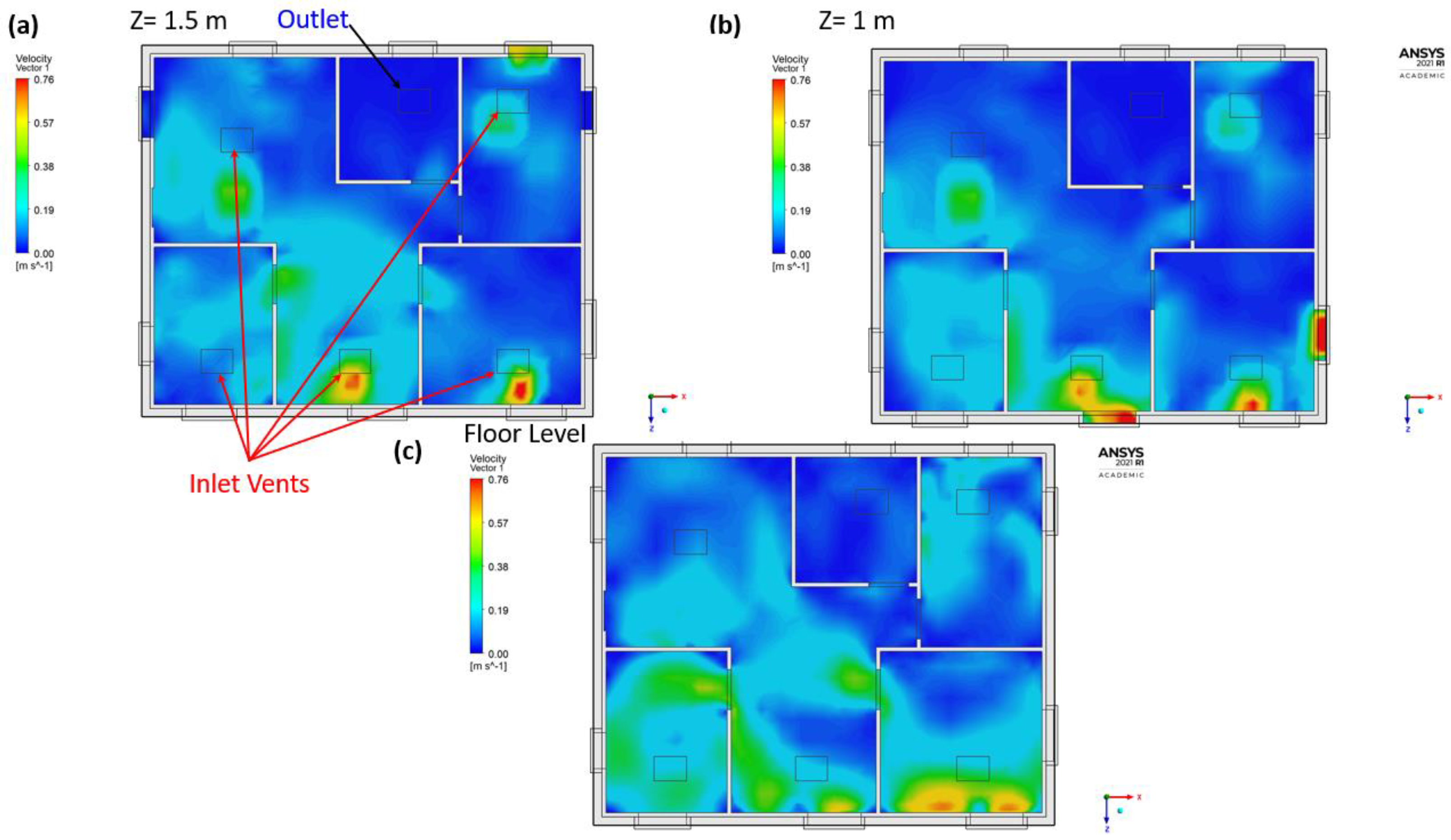
The results, shown in Figure 5, indicate that the velocity ranges from 0 m/s to 0.76 m/s for the fluid body as shown at three different planes: the finished floor level; 1 m above the finished floor level; and 1.5 m above the finished floor level. The velocity contours show a good distribution of air flow going to the bedrooms, with increased velocity at the centre of the house, venting outside (exhausting) via the bathroom. The outcome of the velocity contours and vectors encourage us to investigate the temperature distribution at the same planes.

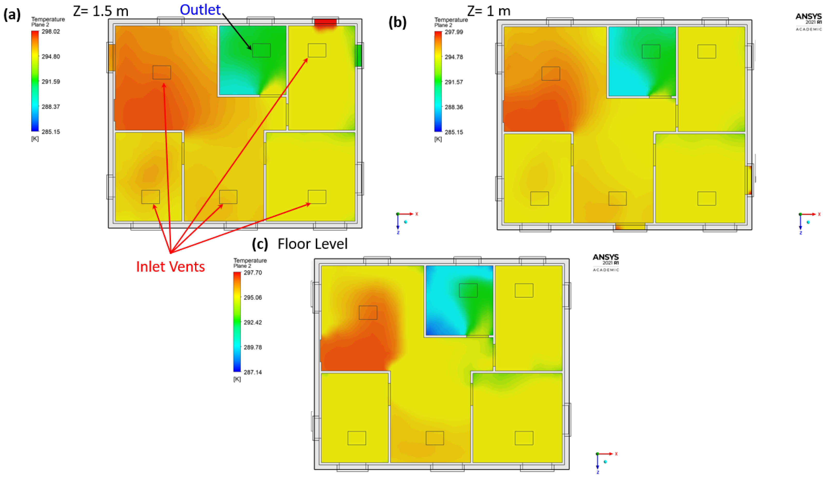
Figure 6 shows the temperature distribution with the duct temperature set to 25 °C (298 K). The results show the temperature ranged between 21 °C and 25 °C (285 K and 298 K). The lower temperature represents the wall temperature, which is to be expected; this was also observed in the thermal images, but the variation was to a much greater extent, as described earlier. The flow rate was designed to improve each room’s thermal comfort, with particular attention given to improving bedroom 2, containing the infant and two adults. The ambient temperatures for the three bedrooms were: 20.82$℃$ in bedroom 1; 24.64$℃$ in bedroom 2; and 24.21$℃$ in bedroom 3. The living room’s average temperature was 20.87$℃$ and the kitchen was 22.03$℃$. Therefore, our proposed system increased the ambient temperature in all rooms, and set them within the range recommended by ASHRAE standard 55-2017 [17], with an average temperature for the house of 21$°\mathrm{C}$, as illustrated in Figure 6.

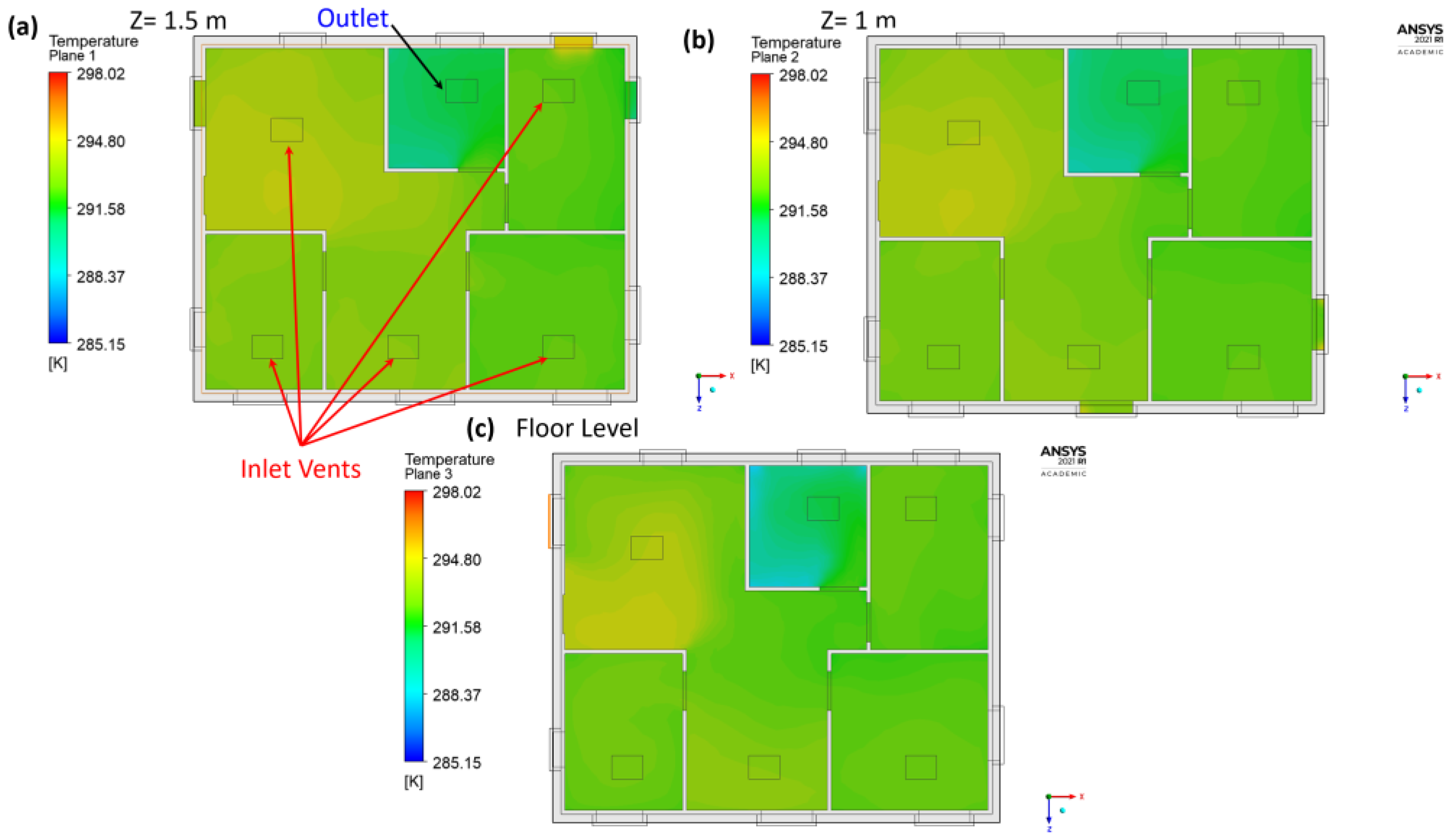
If, alternatively, the inlet temperature was set to 20$°\mathrm{C}$, consistent with the New Zealand Healthy Homes Standards 2019, then the system performs worse in terms of overall temperature. However, the Healthy Homes Standards 2019 [7] require that the main living area be heated to, or above, 18$°\mathrm{C}$ [23]. As shown in Figure 7, the main living room would meet the standard, but the other bedrooms would be lower in temperature.

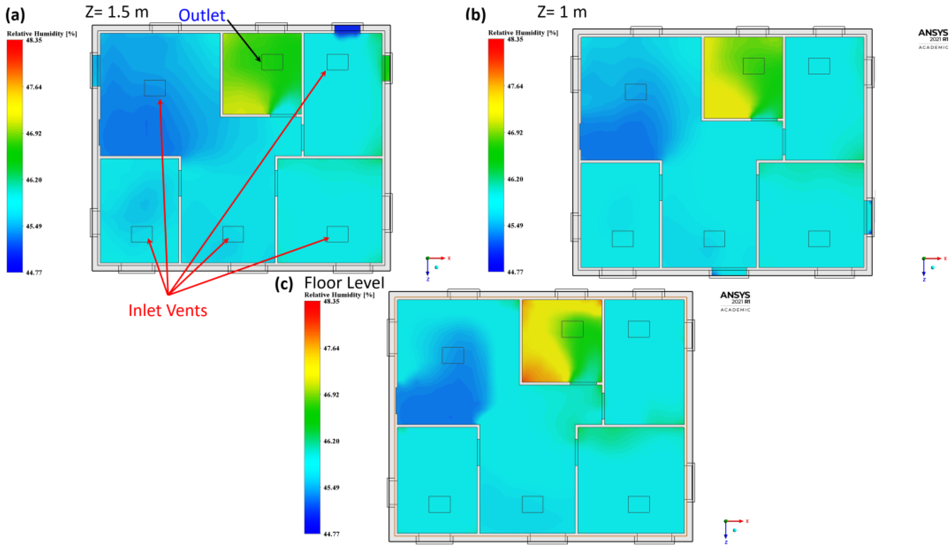
Figure 8 shows the relative humidity profile in the house, at the heights: 0.1 m, 1 m and 1.5 m from the finished floor level. The results show a huge improvement to this IEQ parameter for each room in the house. The average relative humidity for all rooms in the house fell below 50% (whereas, in the house with no intervention, these readings were above 70%). The bathroom had the highest relative humidity (around 48%) reflecting that it is the ventilation room, and assuming that the window is kept open.

The results for the proposed system can be further assessed using the PMV (predicted mean vote) and PPD (predicted percentage dissatisfied) thermal comfort parameters [24,25]. The PMV is an index used to predict how occupants of an indoor space will vote in terms of their thermal sensation. The PMV scale ranges from $-3$ (cold) to $+3$ (hot) and can be embedded into ANSYS-CFX [10,13] using the user CEL (in the C programming language) function with the PMV calculation described in Equation (6) below [13].

$$\begin{gathered} PMV=\left(0.303 e^{\left(-0.036 \mathrm{M}+0.028\right)}\right)*\left\{\left(M-V\right)-3.96\times {10}^{-8}{f}_{cl}\left[{\left(T_{cl}+273\right)}^4-{\left(T_r+273\right)}^4\right]-f_{cl}{h}_c\left(T_{cl}-T_a\right)- \\ 3.05\left[5.73-0.007\left(M-W\right)-p_a\right]-0.42\left[\left(M-W\right)-58.15\right]-0.0173M\left(5.87-p_a\right)-0.0014M\left(34-T_a\right)\right\} \end{gathered}$$

(6)

$$T_{cl}=35.7-0.028\left(M-W\right)-R_{cl}\{39.6\times {10}^{-9}{f}_{cl}\left[{\left(T_{cl}+273\right)}^4-{\left(T_r+273\right)}^4\right]+f_{cl}{h}_c\left(T_{cl}-T_a\right)\}$$

where M is the metabolic value, equal to 60 W/m², or 1.0 met, reflective of non-exertion in activities. Aspects of the body are incorporated, such as $W$ for weight of the person, $f_{cl}$ to reflect the body’s surface area ratio, $T_{cl}$ to reflect the clothing’s surface temperature, $I_{cl}$ is the thermal resistance of the clothing (m²k/W), and $R_{cl}$ reflects the thermal insulation afforded by the clothing (set to 0.1555$I_{cl}$). The coefficient of convective heat transfer is $h_c$, air temperature is $T_a$ (°C) and the mean radiant temperature is $T_r$ (°C). Relative air velocity is given by $v$ (m/s), and $p_a$ is the water vapour’s partial pressure (as per the saturation curve).

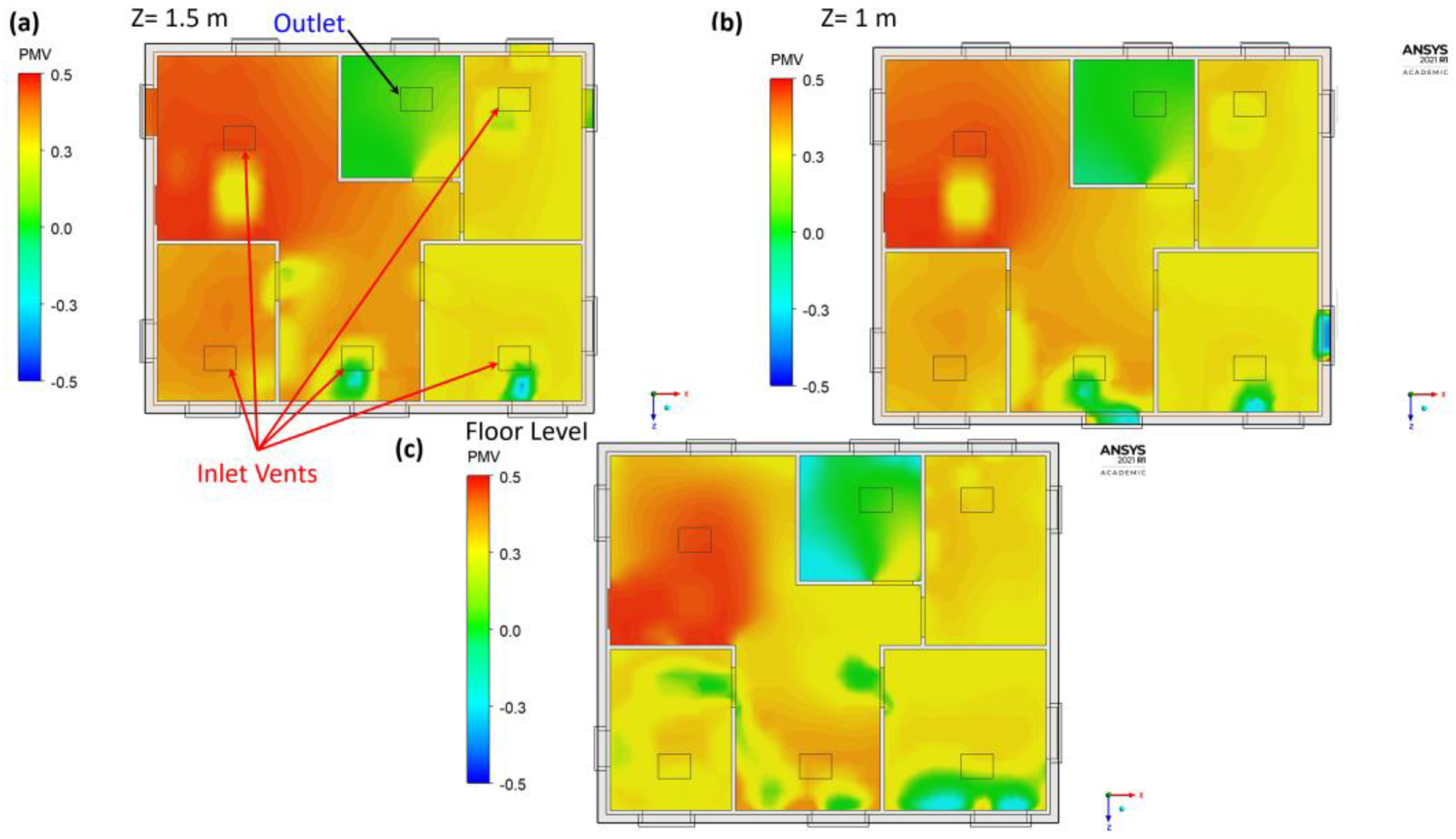
Figure 9 presents our results for the PMV in the house, where the scale on the side shows that all values for PMV were between $-0.5$ and $+0.5$, indicating very good performance in relation to thermal comfort. The highest PMV score was $+0.44$ (in the kitchen) and the lowest was $-0.11$, occurring at the windows and bathroom (venting area) for the house based on the input of 25$℃$ and relative humidity of 45%. Importantly, the bedrooms were in the slightly warm range, which is preferable, particularly for young children.

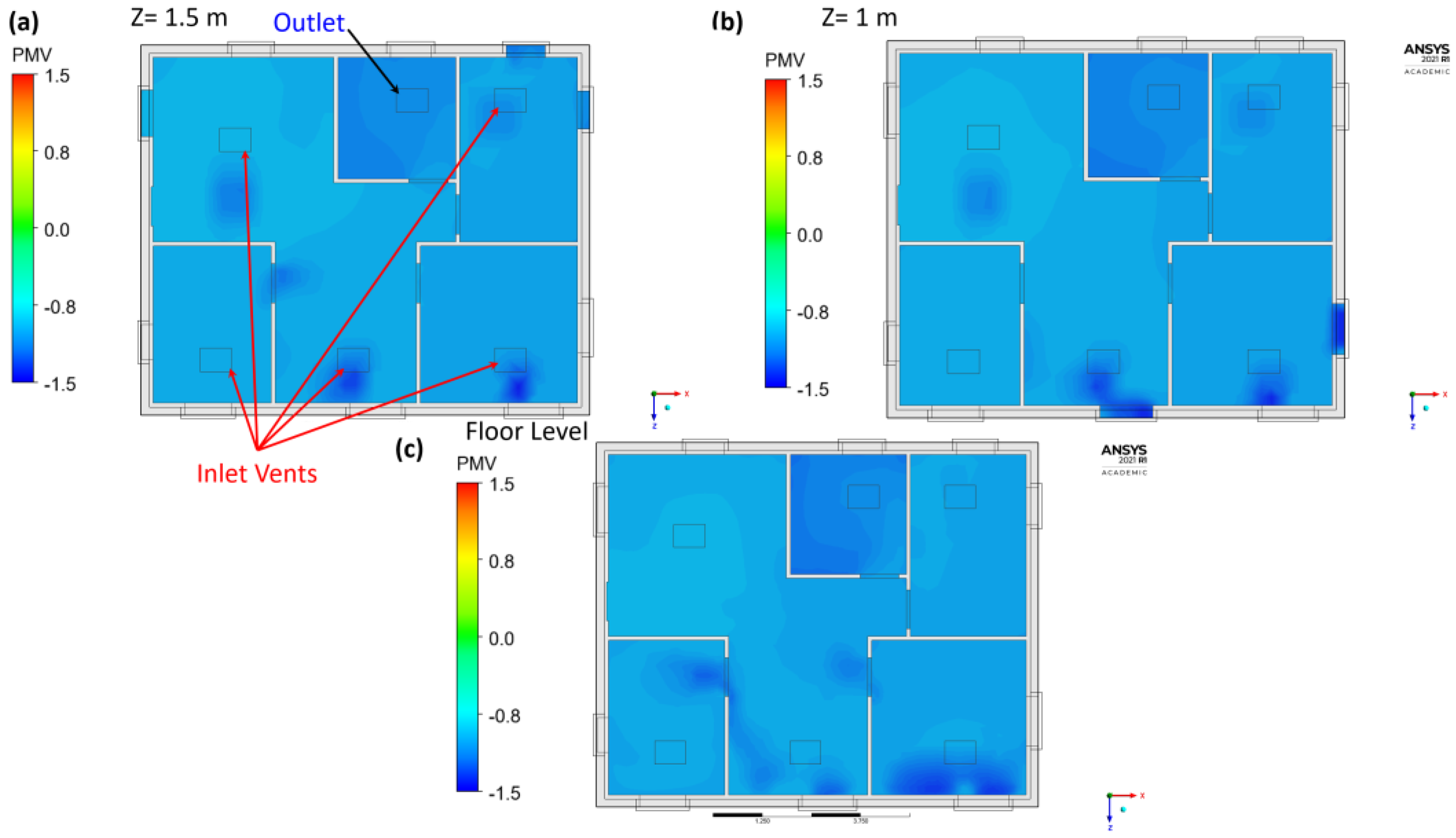
Figure 10 shows the PMV when heating the inlet air to 20$℃$ and relative humidity 45%. The living room performs acceptably (shown by the lighter blue areas), but the bedrooms are colder, indicating more occupants feeling the temperature was colder than they might prefer.

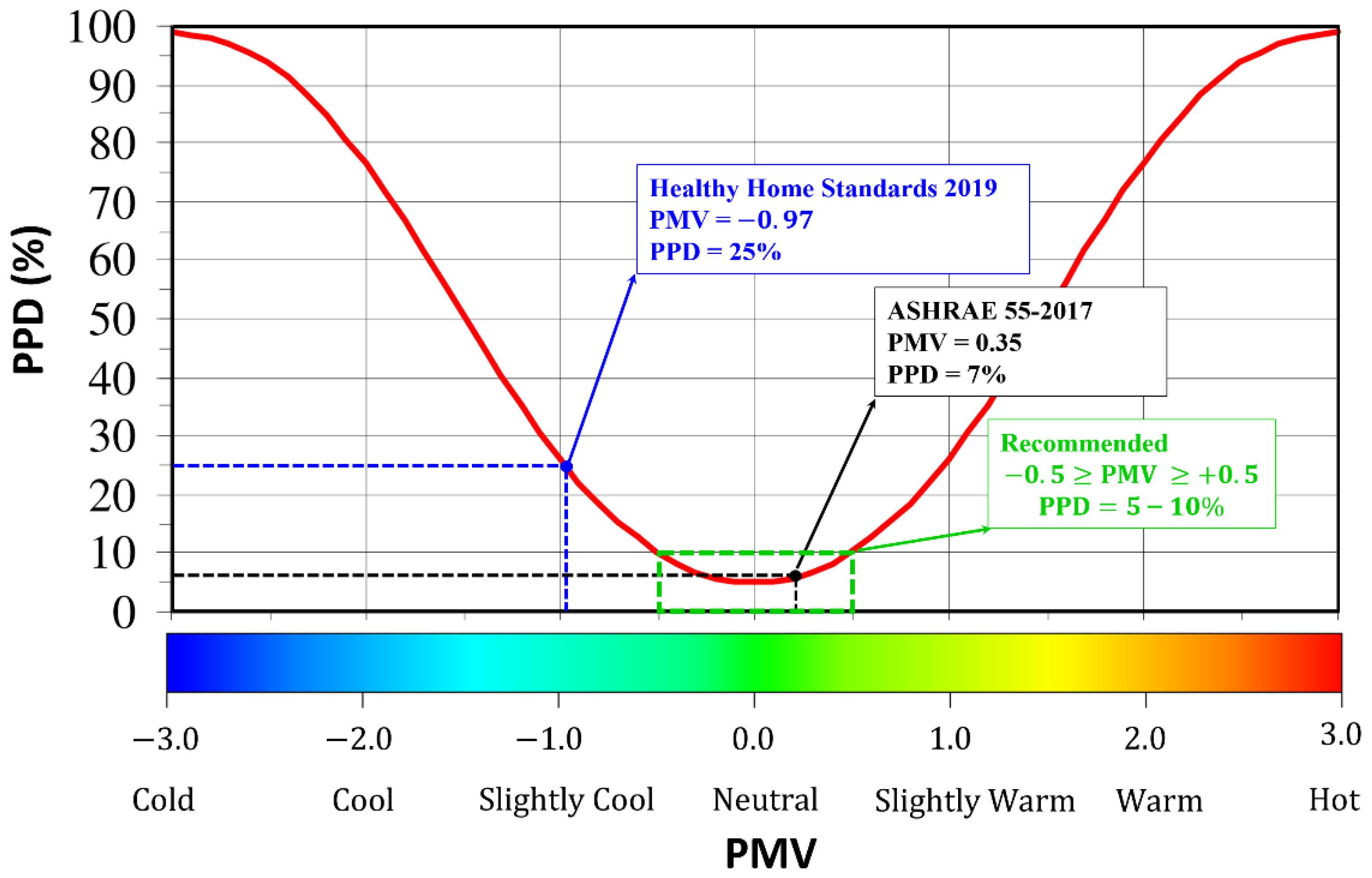
The PPD indicates what percentage of the occupants would not be satisfied with the thermal comfort in the given space. It never reaches zero, as differences in preferred levels of heat and metabolic rate mean the same temperature in the room will not perfectly satisfy all occupants. However, a higher PPD means the room is deemed too hot or too cold for a larger proportion of its occupants. ASHRAE Standard 55-2017 considers a PPD of under 10% reflects an acceptable level of thermal comfort. 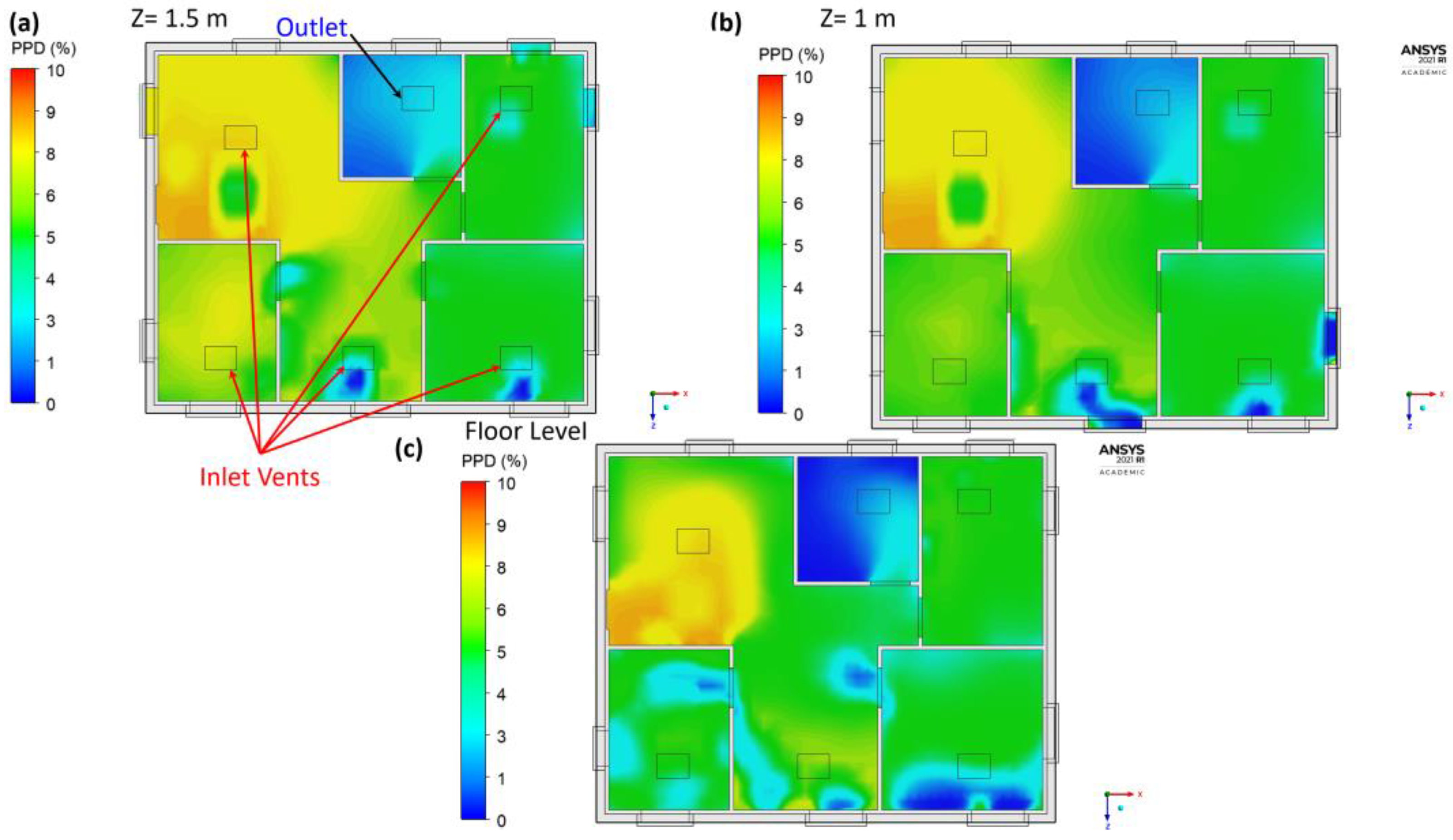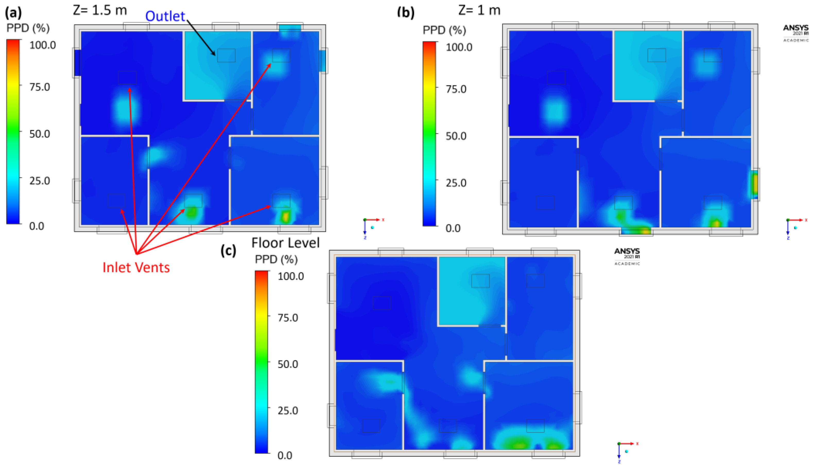Figure 11 shows the PPD contours for the house assessed based on both standards EN ISO 7730 and ASHRAE 55-2017 using Equation (7).

$$PPD=100-95e^{\left(-0.03353 PM{V}^4-0.2179 PM{V}^2\right)}$$

(7)

The CFD results show that when the inlet temperature is heated to 25$℃$, the PPD for the house of between 5% and 9%, which is within the acceptable range, given the current temperature and relative humidity. Therefore, the proposed system shows significant improvement of the indoor thermal conditions for the occupants.

When using the lower inlet temperature of 20$℃$, consistent with the Healthy Homes Standards 2019, the PPD values are much higher, as evidenced by Figure 12, where the scale shows much higher values of PPD, with an average PPD of 25%. This means a significant proportion of occupants may find the temperature too cold in the house. Consequently, although the living room can reach the minimum value of 18$℃$, as set out by the Healthy Homes Standards 2019, the overall temperatures in the house’s living spaces may result in less satisfaction with thermal comfort for the household’s occupants.

Figure 13 shows the comparison between the thermal comfort performance of the two inlet temperature sets (25$℃$, and 20$℃$). The optimal location is the area outlined in green in Figure 12, with a PMV of $\pm 0.5$, and a PPD of 10% or less. Running the system with the inlet heat of 25$℃$ and relative humidity 45% locates comfortably within this green region of thermal comfort, whereas using a lower inlet temperature of 20$℃$ leaves the house outside of the ideal zone of thermal comfort. This indicates that targeting a temperature of 18$℃$ for the main living area, in a ducted heat pump system, may leave the rest of the household uncomfortable (slightly cold).

5. Conclusions

Poor quality housing represents a form of deprivation that disproportionately impacts those from low income and marginalised communities. Poor quality housing generates indoor spaces which have poor indoor environmental quality (IEQ) measures, such as high relative humidity, low temperature, and are associated with higher incidence of respiratory illness, particularly among infants and young children. In this paper we presented a sample house from a collection of houses surveyed in the Manukau, Auckland region of New Zealand, which is an area with lower average income. This case-study house performed poorly in terms of most IEQ measures: all rooms were colder than recommended for indoor living spaces; the relative humidity was higher than recommended, and the thermal image results showed significant cold-spots and variations in temperature in living spaces; however, the moisture content of the walls was in the acceptable range. We then simulated the effect of a ducted heat pump if it were applied to this house. The simulation for this proposed HVAC system, conducted in ANSYS CFX 2021 R1 showed that when the system used an inlet temperature of $25 ℃$ and relative humidity 45%, it was capable of lifting the indoor temperature to above $21 ℃$, including at the walls of the room, thereby eliminating cold spots and improving thermal comfort, particularly in the living areas (bedrooms and living room). The proposed system also reduced relative humidity to below 50%, which would conform to the acceptable range defined by ASHRAE Standard 55-2017, and improved the performance of the house in terms of the PMV and PPD measures of thermal comfort. When using a lower inlet temperature of $20℃$ to lift the living room’s temperature to the target of $18 ℃$, the rest of the house performed worse in terms of thermal comfort, and it was likely the occupants would not be satisfied with the thermal comfort.

References

1. Stats, N.Z. Housing Costs Rise, Impact Felt Strongly by Renters. 2022. Available online: https://www.stats.govt.nz/news/housing-costs-rise-impact-felt-strongly-by-renters/ (accessed on 8 September 2022).
2. Stats, N.Z. Living in a Crowded House: Exploring the Ethnicity and Well-Being of People in Crowded Households. 2018. Available online: https://www.stats.govt.nz/assets/Uploads/Reports/Living-in-a-crowded-house-exploring-the-ethnicity-and-well-being-of-people-in-crowded-households/living-in-a-crowded-house-exploring-the-ethnicity-and-well-being-of-people-in-crowded-households.pdf (accessed on 8 September 2022).
3. Stats, N.Z. 2018 Census Place Summaries, Manukau Central. 2018. Available online: https://www.stats.govt.nz/tools/2018-census-place-summaries/manukau-central (accessed on 8 September 2022).
4. Islam, M.; Sultana, Z.Z.; Iqbal, A.; Ali, M.; Hossain, A. Effect of in-house crowding on childhood hospital admissions for acute respiratory infection: A matched case-control study in Bangladesh. Int. J. Infect. Dis. 2021, 105, 639–645. [Google Scholar] [CrossRef] [PubMed]
5. Cardoso, M.; Cousens, S.; de Góes Siqueira, L.; Alves, F.; D’Angelo, L. Crowding: Risk factor or protective factor for lower respiratory disease in young children? BMC Public Health 2004, 4, 19. [Google Scholar] [CrossRef] [PubMed] [Green Version]
6. Ingham, T.; Keall, M.; Jones, B.; Aldridge, D.; Dowell, A.; Davies, C.; Crane, J.; Draper, J.B.; Bailey, L.O.; Viggers, H.; et al. Damp mouldy housing and early childhood hospital admissions for acute respiratory infection: A case control study. Thorax 2019, 74, 849–857. [Google Scholar] [CrossRef] [PubMed] [Green Version]
7. Te Whatu Ora, Health New Zealand. Healthy Home Initiative. 2022. Available online: https://www.tewhatuora.govt.nz/keeping-well/healthy-homes-initiative/ (accessed on 8 September 2022).
8. Morton, S.; Lai, H.; Walker, C.; Cha, M.J.; Smith, M.A.; Marks, E.; Pillai, M.A. Keeping Our Children Warm and Dry: Evidence from Growing Up in New Zealand. 2021. Available online: https://www.branz.co.nz/pubs/research-reports/er58/ (accessed on 7 October 2021).
9. Mora Pérez, M.; López-Patiño, G.; Guillén Guillamón, I.; López Jiménez, P. CFD Model of Thermal and Velocity Conditions in a Particular Indoor Environment. 2022. Available online: http://hdl.handle.net/10251/43377 (accessed on 12 September 2022).
10. Al-Rawi, M. The thermal comfort sweet-spot: A case study in a residential house in Waikato, New Zealand. Case Stud. Therm. Eng. 2021, 28, 101530. [Google Scholar] [CrossRef]
11. Wahhad, A.; Adam, N.; Sapuan, S. Comparison of numerical simulation and experimental study on indoor air quality of air-conditioned office building in desert climate. Int. J. Automot. Mech. Eng. 2015, 12, 3109–3124. [Google Scholar] [CrossRef]
12. Raczkowski, A.; Suchorab, Z.; Brzyski, P. Computational fluid dynamics simulation of thermal comfort in naturally ventilated room. Matec Web Conf. 2019, 252, 04007. [Google Scholar] [CrossRef]
13. Al-Rawi, M.; Al-Jumaily, A.M.; Lazonby, A. Did You Just Cough? Visualization of Vapor Diffusion in an Office Using Computational Fluid Dynamics Analysis. Int. J. Environ. Res. Public Health 2022, 19, 9928. [Google Scholar] [CrossRef] [PubMed]
14. Zhong, F.; Calautit, J. An Integrated Cooling Jet and Air Curtain System for Stadiums in Hot Climates. Atmosphere 2020, 11, 546. [Google Scholar] [CrossRef]
15. Hormigos-Jimenez, S.; Padilla-Marcos, M.; Meiss, A.; Gonzalez-Lezcano, R.; Feijó-MuÑoz, J. Experimental validation of the age-of-the-air CFD analysis: A case study. Sci. Technol. Built Environ. 2018, 24, 994–1003. [Google Scholar] [CrossRef]
16. Auckland Council. The Auckland Plan. 2022. Available online: https://www.aucklandcouncil.govt.nz/plans-projects-policies-reports-bylaws/our-plans-strategies/auckland-plan/Pages/default.aspx (accessed on 18 September 2022).
17. ASHRAE Standard 55-2017. ASHRAE Technical FAQ. 2017. Available online: https://www.ashrae.org/File%20Library/Technical%20Resources/Technical%20FAQs/TC-02.01-FAQ-92.pdf (accessed on 8 September 2022).
18. Mayo Clinic. Humidifiers: Why You Might Need Them. 2022. Available online: https://www.mayoclinic.org/diseases-conditions/common-cold/in-depth/humidifiers/art-20048021 (accessed on 14 September 2022).
19. Al-Rawi, M.; Farid, M.M.; Jones, R.J.; Louie, K. Evaluation of a Polyester Filter and UV Light (PFUV) Dehumidifier to Improve Indoor Environmental Quality: Preliminary Results. Sustainability 2022, 14, 4504. [Google Scholar] [CrossRef]
20. 2022. Available online: https://www.instrumart.com/assets/MMS2-manual.pdf (accessed on 14 September 2022).
21. ANSI/ASHRAE Standard 62.1 and 62.2. The Standard for Ventilation and Indoor Air Quality. 2022. Available online: https://www.ashrae.org/technical-resources/bookstore/standards-62-1-62-2 (accessed on 17 September 2022).
22. Latif, H.; Rahnama, S.; Maccarini, A.; Bradshaw, C.R.; Hultmark, G.; Nielsen, P.V.; Afshari, A. Precision Ventilation for an Open-Plan Office: A Study of Variable Jet Interaction between Two Active Chilled Beams. Sustainability 2022, 14, 11466. [Google Scholar] [CrossRef]
23. Heating Standard. 2022. Available online: https://www.tenancy.govt.nz/healthy-homes/heating-standard/ (accessed on 17 September 2022).
24. Tuck, N.W.; Zaki, S.A.; Hagishima, A.; Rijal, H.B.; Zakaria, M.A.; Yakub, F. Effectiveness of free running passive cooling strategies for indoor thermal environments: Example from a two-story corner terrace house in Malaysia. Build Environ. 2019, 160, 106214. [Google Scholar] [CrossRef]
25. Aqilah, N.; Zaki, S.A.; Hagishima, A.; Rijal, H.B.; Yakub, F. Analysis on electricity use and indoor thermal environment for typical air-conditioning residential buildings in Malaysia. Urban Clim. 2021, 37, 100830. [Google Scholar] [CrossRef]
Figure 1. The thermal images for the house surveyed with four adults and one infant aged nine months old: (a) bedroom 1; (b) bedroom 2; (c) bedroom 3; (d) living room; and (e) kitchen. The red/orange colors in the image represent warmer areas and blue colors represent colder areas.
Atmosphere 13 01703 g001
Figure 2. The computational domain with boundary conditions showing the house model containing the ducted heat pump system with the inlet and outlet vents (a) the iso-view and (b) the top view.
Atmosphere 13 01703 g002aAtmosphere 13 01703 g002b
Figure 3. (a) The mesh geometry for the house (top-view), (b) the quality of the mesh showing the skewness and (c) the element quality.
Atmosphere 13 01703 g003
Figure 4. Computational model validation for the measured temperature and relative humidity.
Atmosphere 13 01703 g004
Figure 5. The analysis of the air velocity contours and vector (top view) in the house at different height (a) 1.5 m, (b) 1 m and (c) (finished) floor level.
Atmosphere 13 01703 g005
Figure 6. Temperature profiles distribution for the house (top view) using ASHRAE 55-2017 inlet temperature 25   at different heights (a) 1.5 m, (b) 1 m, and (c) the (finished) floor.
Atmosphere 13 01703 g006
Figure 7. Temperature profiles distribution for the house (top view) using Healthy Home standards 2019 inlet temperature 20   at different heights (a) 1.5 m, (b) 1 m, and (c) the (finished) floor.
Atmosphere 13 01703 g007
Figure 8. Relative humidity (%) profiles distribution for the house (top view) at different heights (a) 1.5 m, (b) 1 m, and (c) the (finished) floor.
Atmosphere 13 01703 g008
Figure 9. The predicted mean vote (PMV) profiles distribution for the house (top view) using ASHRAE 55-2017 inlet temperature 25   at different heights (a) 1.5 m, (b) 1 m, and (c) the (finished) floor.
Atmosphere 13 01703 g009
Figure 10. The predicted mean vote (PMV) profiles distribution for the house (top view) using Healthy Home standards 2019 inlet temperature 20   at different heights (a) 1.5 m, (b) 1 m, and (c) the (finished) floor.
Atmosphere 13 01703 g010
Figure 11. The predicted percentage dissatisfied (PPD) profiles distribution for the house (top view) using ASHRAE 55-2017 inlet temperature 25   at different heights (a) 1.5 m, (b) 1 m, and (c) the (finished) floor.
Atmosphere 13 01703 g011
Figure 12. The predicted percentage dissatisfied (PPD) profiles distribution for the house (top view) using Healthy Home standards 2019 inlet temperature 20   at different heights (a) 1.5 m, (b) 1 m, and (c) the (finished) floor.
Atmosphere 13 01703 g012
Figure 13. The PMV and PPD for the Healthy Home standards 2019 and for the ASHRAE 55-2017.
Atmosphere 13 01703 g013