
Equatorial Plasma Bubbles: A Review

Indian Institute of Geomagnetism, Navi Mumbai 410218, India
Atmosphere 2022, 13(10), 1637; https://doi.org/10.3390/atmos13101637
Submission received: 22 August 2022
/
Revised: 25 September 2022
/
Accepted: 27 September 2022
/
Published: 8 October 2022
(This article belongs to the Special Issue Ionospheric and Magnetic Signatures of Space Weather Events at Middle and Low Latitudes: Experimental Studies and Modelling)
Abstract
:The equatorial plasma bubble (EPB) phenomenon is an important component of space weather as the ionospheric irregularities that develop within EPBs can have major detrimental effects on the operation of satellite-based communication and navigation systems. Although the name suggests that EPBs occur in the equatorial ionosphere, the nature of the plasma instability that gives rise to EPBs is such that the bubbles may extend over a large part of the global ionosphere between geomagnetic latitudes of approximately ±15°. The scientific challenge continues to be to understand the day-to-day variability in the occurrence and characteristics of EPBs, such as their latitudinal extent and the development of irregularities within EPBs. In this paper, basic theoretical aspects of the plasma processes involved in the generation of EPBs, associated ionospheric irregularities, and observations of their characteristics using different techniques will be reviewed. Special focus will be given to observations of scintillations produced by the scattering of VHF and higher frequency radio waves while they propagate through ionospheric irregularities associated with EPBs, as these observations have revealed new information about the non-linear development of Rayleigh–Taylor instability in equatorial ionospheric plasma, which is the genesis of EPBs.
1. Introduction
Manifestations of phenomena associated with space weather, unlike those linked with terrestrial weather, generally require specialized instruments for observation. An equatorial plasma bubble (EPB) is one such phenomenon, which occurs in the post-sunset equatorial and low-latitude ionosphere. An EPB refers to a region extending vertically upwards from the bottom side of the equatorial F region, with significantly lower plasma density than the background ionosphere. It is aligned with the geomagnetic field so that it may be stretched to hundreds of kilometers in the magnetic north–south direction, while it may have a magnetic east–west extent of tens of kilometers along the bottom side of the equatorial F region. An EPB tends to develop a smaller-scale irregular structure as it rises above the dip equator, and these irregularities are also field-aligned. Usually, several EPBs develop almost simultaneously at a particular longitude, sometimes resulting in a highly structured post-sunset low-latitude ionosphere in a particular longitude sector. Irregular plasma density structures associated with equatorial plasma bubbles (EPBs) are often referred to as equatorial spread F (ESF) irregularities. The term ESF came into existence after certain features were seen in ionogram traces obtained from ionosonde observations [1]. One such feature was the presence of a range of virtual heights for the reflecting regions in the ionogram, as the ionosonde frequency was changed, instead of a thin line representing a particular virtual height of reflection for the signal at a particular frequency. This came to be known as ‘range spread’. The other feature that is sometimes seen is a spread at the high frequency end of the ionogram trace, at a fixed virtual height, such that the critical frequency (foF2) could not be determined. This is referred to as ‘frequency spread’. Booker and Wells [2] suggested that these features appeared on ionograms, obtained at an equatorial station, due to scattering of the ionosonde radio signal by electron density variations associated with irregularities in the equatorial ionosphere. Such irregularities also scattered radio waves emitted by radio stars and were recorded on the ground, giving rise to fluctuations or scintillations in the intensity of the recorded signal [3,4]. Once the launch of artificial satellites ushered in the ‘Space age’, radio signals transmitted from these satellites were used to obtain a global picture of the occurrence of ionospheric scintillations [5]. In the equatorial and low-latitude regions, strong scintillations were recorded only during post-sunset hours [6]. Ionosonde observations of the ESF phenomenon also showed it to be a nighttime phenomenon. Theoretical investigations on scintillations have shown that ionospheric irregularities with scale sizes in the intermediate range (100 m to a few km) may give rise to strong scintillations on VHF to L-band trans-ionospheric radio signals. Such irregularities are generated in the course of the non-linear development of EPBs when they become highly structured. Many modern-day technologies are greatly dependent on space-based navigation systems, such as the Global Navigation Satellite Systems (GNSS), which transmit L-band signals. Scintillations on these signals caused by intermediate-scale irregularities within EPBs may cause loss of signal and loss of lock when a ground-based receiver tries to record the signal from a satellite as it comes into view. This is sometimes highly detrimental to the operation of satellite-based communication and navigation systems. Therefore, EPBs are considered to be an important component of space weather and continue to be studied vigorously even after so many decades since their existence was discovered.
It was first proposed by Dungey [7] in 1956 that growth of the collision-dominated Rayleigh–Taylor (R–T) instability on the bottom side of the post-sunset equatorial ionosphere was responsible for the development of ESF irregularities. Strong coherently backscattered signals during ESF conditions observed at the Jicamarca Radar Observatory (JRO) led to the systematic study of ESF irregularities at this facility. The JRO became operational in the early 1960s with the aim of studying ionospheric electron densities, temperatures, and ion composition using incoherently scattered radar signals. Incoherent scattering of the transmitted radar signal in the ionosphere is due to thermal fluctuations in electron density, which are always present and give rise to a weak scattered signal. Thus, an incoherent scatter radar requires a powerful transmitter and a large antenna. In the presence of ESF irregularities, a strong backscattered radar signal was observed, and this was attributed to coherent scattering by the ESF irregularities. This was considered to be Bragg scattering by irregularities of a particular wavelength depending on the radar signal frequency. Thus, the irregularities that caused backscattering of vertically propagated signals at the JRO were the ones with vertical wave vectors corresponding to a wavelength of 3 m, which is half the wavelength of the radar signal. Measurements made by such radars are displayed as two-dimensional maps of the intensity of the backscattered signal as a function of altitude and time. Observations at the JRO showed that echoes also came from regions above the peak of the F layer, indicating the presence of ESF irregularities on the top side of the post-sunset equatorial F-layer, where the plasma density gradient is downward. Farley et al. [8] pointed out that Dungey’s theory [7] could not explain these observations of top-side ESF irregularities. Range–time–intensity (RTI) maps obtained at the JRO showed plume-like features, which led Woodman and LaHoz [9] to postulate that a large scale perturbation on the unstable bottom side of the post-sunset equatorial ionosphere could develop non-linearly into a low-density (compared to the background plasma density) plasma bubble, which could rise to the top side of the equatorial ionosphere, which is otherwise stable. A theoretical breakthrough put this idea on firm ground when Scannapieco and Ossakow [10] carried out numerical simulation of the non-linear development of collisional R–T instability where an equatorial plasma-depleted bubble was shown to rise to the linearly stable top side of the equatorial ionosphere. The R–T instability involves the interchange of entire geomagnetic flux tubes; therefore, the EPBs would be highly elongated in the direction of the geomagnetic field [11]. A fully steerable radar, ALTAIR, located in the Kwajalein Atoll in the Marshal Islands at a magnetic dip latitude of 4.3° N was used by Tsunoda [12] to demonstrate the geomagnetic field-aligned nature of EPBs. After decades of study using various observation techniques, and with substantial progress in the numerical simulation of the non-linear development of EPBs and the structures within them, the challenge of understanding day-to-day variability in the occurrence and characteristics of EPBs still remains.
After this introduction to the origin of the term ‘equatorial plasma bubble’ (EPB), in the next section of this paper, the contributions of various techniques to the observation of the different characteristics of EPBs and associated ionospheric irregularities are described. In the third section, theoretical aspects of the linear and non-linear development of R–T instability, as applicable to the generation of EPBs and some of the associated irregularities, are discussed. Although observations of EPBs, associated irregularities, and theoretical developments are described under different sections, in reality, many developments in both areas are closely linked. These connections will be pointed out as they arise in the discussion. The fourth section is devoted to a closer look at more recent observational and theoretical results, with a focus on new results obtained from analysis of ionospheric scintillation data and new three-dimensional simulations of the non-linear evolution of EPBs. This section summarizes the current scenario regarding EPBs and indicates some of the areas where future studies are required.
2. Observations of EPBs and Associated Irregularities
It has already been described in the Introduction how ionosonde observations of range and frequency spread indicated the presence of irregularities in the equatorial and off-equatorial low-latitude ionosphere during post-sunset hours and gave rise to the generic term ‘Equatorial Spread F’ (ESF). However, there has been no theoretical investigation towards establishing a relationship between the features of ESF observed by an ionosonde and the characteristics of irregularities that give rise to spread F on ionograms. As such, scale sizes of the irregularities that produce range or frequency spread on ionograms have not been established, unlike the situation with coherently backscattered radar signals or ionospheric scintillations, where it is known theoretically that irregularities of certain scale sizes are involved in their production. Nevertheless, ionosonde observations are still widely used to indicate the presence of irregularities in the post-sunset equatorial and low-latitude ionosphere [13]. While in situ measurements by rocket- or satellite-borne instruments yield information about the various scale sizes present in the plasma density structures encountered in their trajectories, steerable radars are also capable of providing a large-scale picture of EPBs. Ground-based observations of ionospheric scintillations on VHF to L-band trans-ionospheric radio signals have been used to extract information about EPB irregularities of intermediate-scale (100 m to a few km). Observations of EPBs using different techniques have established that the plasma density structures associated with EPBs span a large range of scale sizes, extending from sub-meter measurements to hundreds of kilometers.
2.1. In Situ Observations Using Rockets and Satellites
In situ plasma density and electric field measurements made by instruments flown on rockets and satellites provide information on variations in plasma density and electric fields over a large range of scale sizes and have therefore been used extensively for spectral studies of the ionospheric irregularities associated with EPBs [14,15,16,17,18,19]. With satellite observations, information is obtained about variations essentially in a horizontal direction, while rocket flights provide information about variations in altitude. Such studies have shown that the one-dimensional spectrum of plasma density variations associated with the ESF irregularities, measured by instruments on board rockets or satellites, has a power-law form. One of the first efforts to study the EPB phenomenon, using plasma density probes on board a rocket, was a multi-instrument investigation involving simultaneous rocket and 50 MHz radar observations in Natal, Brazil [20]. In this experiment, a sounding rocket was launched during ESF conditions at nighttime. Plasma density probes on board detected strong fluctuations in plasma density below the F layer peak, and a large bite out in plasma density just below the peak. This was followed by optical observations of a barium cloud released from the rocket, and radar observations of a weak patch of irregularities moving radially away. The combined observations led the authors to suggest that EPBs move upwards after their generation in the bottom side of the post-sunset equatorial F region [20]. In situ measurements of plasma density using probes on board rockets and satellites, in conjunction with radar observations of backscattered radio signals, have provided the connection between plumes observed in radar RTI maps and EPBs. In an early campaign, a rocket carrying high-resolution plasma density probes, electric field probes, and other instruments was launched so that it would penetrate a well-developed plume above the equatorial F region peak, as seen in the RTI maps obtained from the ALTAIR radar [21]. The rocket data provided an altitude profile of plasma density variations associated with the present irregularities and their spectral characteristics in the vertical direction. In another coordinated study, the east–west profile of ion density variations within EPBs, measured in situ at an altitude of about 373 km by an ion drift meter on board the Atmospheric Explorer E (AE-E) satellite, was compared with the backscatter plume obtained from the ALTAIR radar [22]. The authors concluded that, in the plane perpendicular to the geomagnetic field, EPBs are vertically elongated, tilted wedges that extend from the bottom side of the equatorial F layer to the top side. Data collected by polar-orbiting satellites of the Defense Meteorological Satellite Program (DMSP) from 1989 to 2002 showed how the occurrence rate of EPBs at the height of the satellites (~840 km) varied with longitude and day of the year, which had an important connection with longitudinal variation of the declination of the main geomagnetic field at the dip equator [23]. Considering the major disruptive role that irregularities that develop within EPBs may play in the operation of satellite-based communication and navigation systems, in 2008 a satellite was launched by the United States Air Force to specifically study this phenomenon. The Communication/Navigation Outage Forecasting System (C/NOFS) satellite, equipped with a suite of instruments, was launched into a low-inclination (13°) orbit with a perigee of 405 km and apogee of 853 km. C/NOFS data have yielded information not only about irregularity spectra [19,24], but also about the zonal drift of plasma inside the EPBs [25].
Magnetic Signatures of EPBs
Some satellites equipped with magnetometers have also allowed for simultaneous measurements of fluctuations in electric fields and magnetic fields associated with EPBs, which has revealed some new features of EPBs and suggests alternate theories for EPBs, which shall be briefly discussed in Section 3. Instruments on board NASA’s Dynamic Explorer 2 (DE 2) satellite measured electric and magnetic field fluctuations associated with EPBs updrafting at supersonic speeds, which led Aggson et al. [26] to suggest that Alfvén waves are launched in the equatorial F region when an EPB starts to grow there and that these waves carry geomagnetic field-aligned currents, which couple the equatorial F region with conjugate E regions at the feet of the geomagnetic field. Coupling of the equatorial F region with conjugate E regions through geomagnetic field lines is the reason that EPBs are a post-sunset phenomenon, as discussed in Section 3. Electric and magnetic field sensors of the Extremely Low Frequency Wave Analyzer instrument on board the Combined Release and Radiation Effects Satellite (CRRES) detected both electrostatic waves with a small magnetic field component and electromagnetic waves propagating in the extraordinary mode within EPBs mostly in the altitude range of 400–500 km [27]. The French microsatellite mission DEMETER (Detection of Electromagnetic Emissions from Earthquake Regions) also detected electromagnetic fluctuations associated with EPBs in regions with plasma density structures of scale sizes 1–10 km, whereas broadband electrostatic fluctuations were observed in regions with structures of 10–100 m in scale [28].
Magnetic field fluctuations associated with EPBs have been studied extensively using data from the high-resolution vector magnetometer on board the German CHAMP (Challenging Minisatellite Payload) satellite launched in 2000 [29,30]. Vector magnetic field measurements provided estimates of fluctuations in the component of the magnetic field parallel to the main geomagnetic field, as well as fluctuations in the components transverse to the main geomagnetic field. The latter could be produced by field-aligned currents. The CHAMP satellite’s orbit was circular and nearly polar, with a high inclination (87.3°) and initial altitude of about 450 km. In situ plasma density measurements made by a planar Langmuir probe (PLP) showed the presence of EPBs at the height of the satellite. An example of the magnetic field fluctuations associated with EPBs that were present around 38° W geographic longitude is shown in Figure 1. On this day, fluctuations with a maximum amplitude of ±4 nT are seen in the magnetic field components transverse to the mean geomagnetic field in the region with the deepest depletions in plasma density. Swarm, ESA’s mission for Earth observation with a constellation of three identical satellites, was launched in 2013. The satellites’ orbits are nearly polar, and they are equipped with vector field magnetometers, Langmuir probes, and thermal ion imagers to measure ion drift, from which electric fields could be estimated [31,32,33]. These observations have been used to study, among other aspects of EPBs, the geomagnetically conjugate characteristics of EPB irregularities [32].
2.2. Radar Observations
The important role played by radar observations at the JRO in the initial characterization of EPBs has been described in the Introduction section. Extensive studies of equatorial spread F using the JULIA (Jicamarca unattended long-time studies of the ionosphere and atmosphere) radar have shown the existence of bottom-type layers which are often present as precursors of the plumes that extend to higher altitudes [34]. Sometimes, the bottom-type layers were precursors to bottom-side layers, which are distinct from the bottom-type layers, being thicker and more structured. Hysell and Burcham [34] found that intermediate-scale plasma depletions often arose from the bottom-side layers and, moving upwards, penetrated through to the top side of the equatorial ionosphere. RTI maps from radars provide detailed pictures of the day-to-day variability in the occurrence of EPBs and in many of their characteristics when they do occur. The challenge is to relate this variability to the state of the post-sunset-coupled ionosphere–thermosphere system, which is determined by forcingsfrom the atmosphere below and the magnetosphere above the ionosphere. An example of the variety displayed by plumes in radar backscatter RTI maps for the post-sunset low-latitude ionosphere is shown in Figure 2. These RTI maps were obtained by the 53 MHz MST (Mesosphere–Stratosphere–Troposphere) radar operating from Gadanki, India, a low-latitude location at a geomagnetic latitude of 6.5° N. On the two consecutive days for which the RTI maps are displayed in Figure 2, different seed perturbations would have initiated the development of EPBs on the bottom side of the equatorial F region after sunset. The EPBs also evolved differently with time and gave rise to plume structures with entirely different characteristics. While comparing the two RTI maps, it has to be kept in mind that the plume structures that appear in an RTI map arise due to backscattering of the radar signal from a succession of EPB structures that drift into the radar’s field of view at different times. Thus, the EPBs on the two days would have been initiated at different locations along the dip equator. Observations using this radar, located away from the dip equator, have indicated the greater presence of multiple plumes compared to those seen in backscatter of a radar signal from meter-scale irregularities at an equatorial location [35]. A 30 MHz radar with scanning capability in a plane perpendicular to the geomagnetic field and an interferometry/imaging system has also been established at Gadanki in order to study drifts and spatial distribution of large- and small-scale irregularities. Observations of F region irregularities with this radar show bottom-type, bottom-side, and plume structures [36] similar to those reported at Jicamarca, an equatorial location [34]. The 47 MHz Equatorial Atmosphere Radar (EAR) located in West Sumatra, Indonesia, at a dip latitude of 10.36° S, has also been used extensively in investigations of ESF irregularities at an off-equatorial location [37]. The steering capabilities of this radar have enabled it to clearly establish the connection between the onset of equatorial F region irregularities and the sunset terminator [38].
2.3. Ionospheric Scintillation Measurements
It has been mentioned in the Introduction that out of the vast range of scale sizes for the structures associated with EPBs, extending over six orders of magnitude, only irregularities with scale sizes in the intermediate range extending from about 100 m to a few km give rise to scintillations on VHF and higher frequency radio signals propagating through the equatorial and low-latitude ionosphere. The reason for this is that maximum contribution to fluctuations in signal amplitude comes from scattering caused by irregularities with scale sizes around the Fresnel scale [39]. The Fresnel scale defined as equals , where is the wavelength of the radio signal and is the average distance of the layer of irregularities from the receiver along the path of the signal. A VHF or higher frequency signal transmitted from a satellite and recorded by a ground receiver is essentially a forward scattered signal, since the scale sizes of the irregularities which give rise to scintillations are in the range of approximately 100 m to a few km, which is much greater than the signal wavelength. In the case of radar observations, the radar signal is backscattered by irregularities of a scale size that is half the signal wavelength. Forward scattering of the signal by ionospheric irregularities produces a pattern of spatially varying intensity on the ground. This pattern moves across a receiver either due to irregularities drifting across the signal path, as in the case of signals transmitted from a geostationary satellite, or due to the signal sweeping across the irregularities as well, as is the case for signals transmitted from orbiting satellites such as the GNSS satellites. This movement of the pattern across a receiver causes the receiver to record a signal with temporally varying amplitude and phase. Thus, ionospheric scintillation data contain a wealth of information about ESF irregularities. This is an inexpensive technique for studying the intermediate-scale irregularities that develop within EPBs and has been used extensively in different longitudinal zones around the globe [5]. Developments in the theory of scintillations and analysis of ionospheric scintillation data have yielded important information about the characteristics and evolution of intermediate-scale irregularities in EPBs [39,40].
2.3.1. Dependence of Scintillation Parameters on Irregularity Characteristics
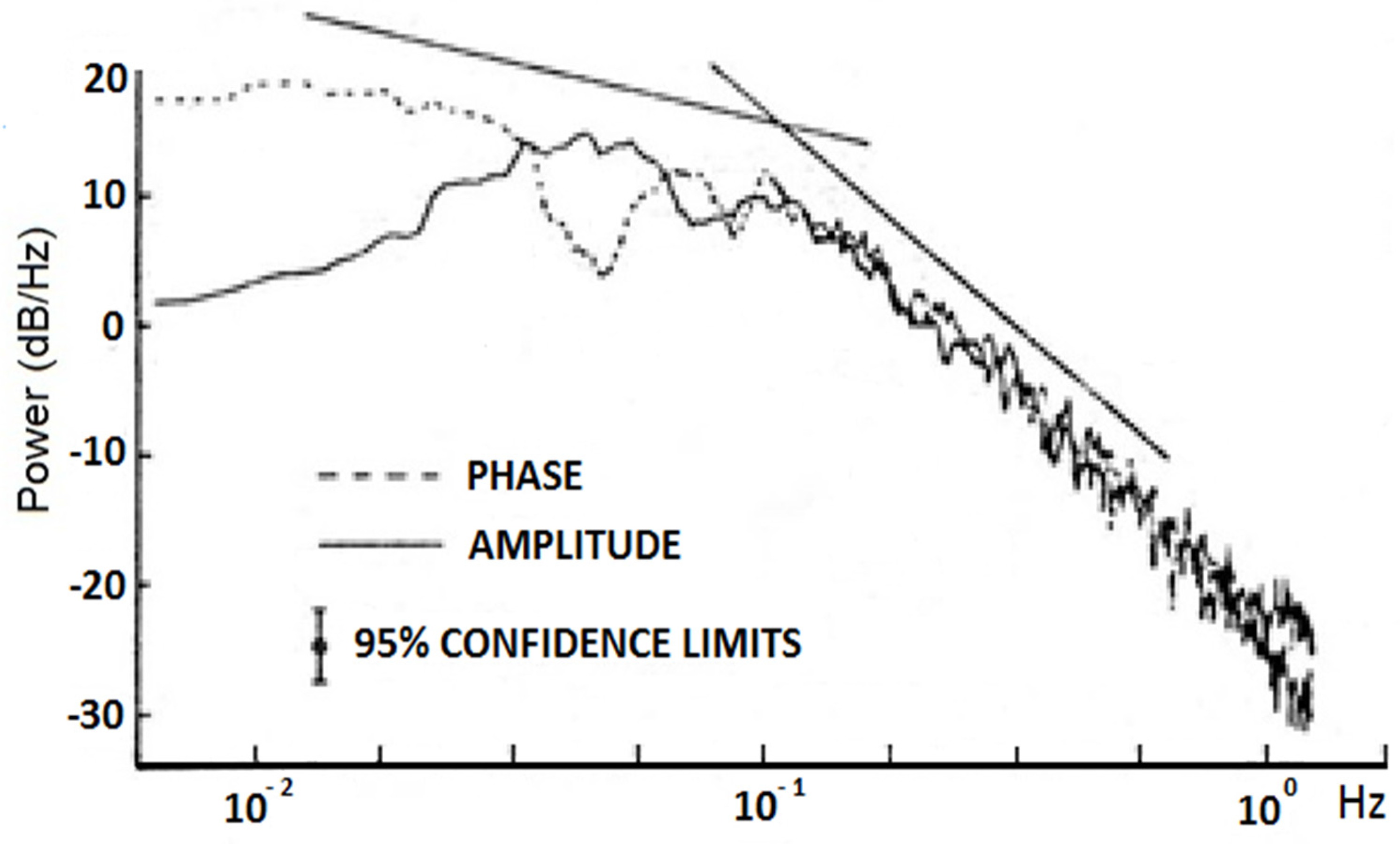
A brief discussion of some of the theoretical aspects of ionospheric scintillations is presented here to make it easier for the reader to understand the relationship between the parameters estimated from scintillation data and irregularity characteristics. This forms the basis for extraction of information about intermediate-scale irregularities in EPBs from scintillation observations [40]. The most commonly used parameter derived from amplitude scintillation data is the index, which is the standard deviation of normalized intensity of the signal and indicates the strength of amplitude scintillations. Scintillations during an interval of time are considered to be weak if < 0.5. In the theory of ionospheric scintillations, a stochastic description of the irregularities is used. Scattering of the radio signal is due to variations in the refractive index of the ionosphere which are directly related to fluctuations in electron density expressed as: , where is the ‘classical radius’ of the electron [39]. It is seen from this relationship that the higher the frequency of the radio signal, the smaller the change in ionospheric refractive index for a particular variation in electron density. Therefore, ionospheric scintillations are expected to be stronger on lower frequency radio signals than on higher frequency signals. The phase screen approximation has been widely used in theoretical investigations of ionospheric scintillations [41]. In this approximation, the layer of irregularities traversed by the radio signal is replaced by a phase-changing screen so that a phase perturbation is imposed on the radio wave as it emerges from the screen. For a two-dimensional phase screen, this phase perturbation has a spatial variation given by , where the two-dimensional vector specifies the location in the screen and is the variation of the total electron content along the signal path to that location which occurs due to the presence of irregularities. After emerging from the phase screen, as the radio waves propagate to a ground receiver, phase perturbation imposed on the incoming radio waves by the irregularities gives rise to amplitude and phase scintillations. As the EPBs and associated irregularities are aligned with the geomagnetic field, which is horizontal at the dip equator, a phase screen varying only in one direction, along the geomagnetic east–west, is often used in modeling scintillations in the equatorial and low-latitude regions. Scintillation characteristics, such as the index, correlation functions, or power spectra, are statistical in nature and are theoretically related to statistical features of the irregularities. In such theories, the stochastic nature of the irregularities is described by their spatial power spectrum [39,40]. Rocket and satellite measurements have shown that one-dimensional spectra of plasma density variations in ESF irregularities have a power-law form, which sometimes show a break in slope [14,15,16,17,18,19]. Scintillations recorded by a receiver are temporal fluctuations which are related to spatial variations in the ground scintillation pattern in the plane of the receiver through the speed with which the pattern moves across the receiver. An example of these power spectra with detrended weak amplitude and phase scintillations on a 140 MHz signal transmitted from the geostationary satellite ATS-6 and recorded at the low-latitude station Ootacamund (geomagnetic latitude: 1.8° N) in India is shown in Figure 3. In agreement with the theory outlined in [39], the spectrum of weak amplitude scintillations displays a broad peak centered on the Fresnel frequency , which is related to the Fresnel scale : , where is the drift speed of the ground scintillation pattern. For an assumed height of the phase screen, may be estimated from [42]. It is seen from Figure 3, as suggested by the theory described in [39], that, at frequencies higher than the Fresnel frequency, spectra of amplitude and phase scintillations follow a power-law, which yields information about the power-law spectrum of intermediate-scale irregularities in EPBs observed at that time [42]. For weak scintillations, spatial scales in the ground scintillation pattern correspond to spatial scales present in the irregularities, and the frequencies in the spectra are related to the spatial scales of the irregularities through . For strong scintillations, roll-off in the power spectra occurs at a higher frequency, as the larger irregularities focus the incident radio waves to produce short-scale variations in intensity in the ground scintillation pattern, and the one-to-one correspondence between irregularity scale size and frequency is lost [39]. It may be noted that phase variations in the recorded signal also include the original phase perturbation imposed by the phase screen, which contains spatial scales much larger than the Fresnel scale. These large-scale phase variations arise due to large-scale irregularities, which are not involved in scattering the radio waves. Therefore, in computing , the standard deviation of phase scintillations, the phase of the received signal must be high-pass filtered to retain only frequencies of the order of or higher than the Fresnel frequency, which depends on . Only then does represent the strength of phase scintillations, which vary throughout a scintillation event in the same manner as [43]. Fluctuations in the phase of the recorded signals may be used effectively in studying the break in slope of the irregularity spectrum, even when the break occurs at a scale size larger than or close to the Fresnel scale, as seen in Figure 3. The distinctly different slopes of the linear fits to the spectra of phase fluctuations over different frequency ranges in this figure indicate a two-component irregularity spectrum and also yield an estimate of the scale size where the break in slope occurs [42].
Measurements of amplitude scintillations on a signal transmitted from a geostationary satellite, and recorded by two ground receivers spaced along a magnetic east–west-oriented baseline, yield better estimates of [44]. As the EPB irregularities are aligned with the geomagnetic field, assumed to be in the direction of the y-axis, spatial variations in the ground scintillation pattern are only present in the magnetic east–west direction, which is taken to be along the x-axis. However, it is necessary to take into account the changes in the ground scintillation pattern with time due to fluctuations in the drift velocity of irregularities. As will be seen in the next section, fluctuations in the drift velocity of the irregularities are an important component of the evolution of the irregularities caused by growth of the R–T instability. These give rise to a decorrelation of the signals recorded by spaced receivers, sometimes resulting in the maximum cross-correlation between the two signals falling well below 1. Therefore, a full correlation technique introduced by Briggs [45] has been used in the analysis of spaced receiver measurements of scintillations caused by EPB irregularities. In order to apply this technique, it is assumed that the space–time correlation function for intensity variations in the ground scintillation pattern is of the following form, considering the -axis to be along the baseline of the receivers, which is in the magnetic east–west direction:
The parameter is referred to as the ‘random’ or ‘characteristic’ velocity in the literature [40]. For the computation of and it is not necessary to know the functional form of , which is only required to be a monotonically decreasing function of its argument, with a maximum when the argument has a value 0: . It is seen from Equation (1) that for separation between the two receivers, as long as is non-vanishing, the argument of never becomes 0, thus the maximum value of is achieved at a time lag of , for which the argument has the lowest value. This maximum value is less than 1. Thus, in addition to , there are three more parameters that may be extracted from spaced receiver scintillation data: , , and . For = 0, this becomes the ususal cross-correlation technique for estimating drifts. The situation with non-vanishing is of interest because it provides an opportunity to study the spatial evolution of the EPB irregularities with time in the non-linear phase of the development of R–T instability. An example of the variation of , , , and through the course of a scintillation event, recorded at the equatorial station Tirunelveli (geomagnetic latitude: 0.2° S) in India on a magnetically quiet day, is shown in Figure 4.
The pattern of local time variations for and shown in Figure 4 is fairly typical for most magnetically quiet days irrespective of how varies, as it is a fundamental characteristic of the development of R–T instability [47,48]. This will be discussed in a later section. The parameters , , and , as computed for each sub-interval of a scintillation event, have also been used in a novel way to determine the functional form of , and hence the dominant spatial scale in the ground scintillation pattern of intensity variations for each sub-interval of the scitillation event. It is seen from Equation (1) that is given by
Although analyzed scintillation data are always a time series, it is necessary to derive information about the spatial variations in signal intensity in the plane of the receiver in order to relate the scintillations to the irregularities. For this purpose, it is seen from Equation (1) that the spatial correlation function for intensity variations in the ground scintillation pattern is given by . Subsequently, according to Equation (2), if is plotted as a function of , it would be equivalent to plotting as a function of the spatial lag . Since the distance between the two receivers, , is known and , , and are computed for each sub-interval from scintillation event data, it is possible to make scatter plots, such as the one in Figure 5, to obtain a picture of how the dominant spatial scale in the ground scintillation pattern of intensity variations evolves with local time, which is related to the development of the irregularities encountered by the radio signal [49]. Evolution of the EPB irregularities with time is dependent on the season and also on the level of ionospheric disturbance due to magnetic storms. Parameters estimated from records of amplitude scintillations on a 251 MHz signal transmitted from a geostationary satellite and recorded by spaced receivers at the equatorial station Tirunelveli during magnetically quiet days of September 2002 have been used in Figure 5. The scatter plot shows that the dominant spatial scale in the intensity variations tends to be shortest around midnight, which has implications for how the intermediate-scale irregularity spectrum develops near the equatorial F region peak [49].
Observations of irregularities associated with EPBs using ionosonde, radar, or the scintillation technique utilize radio waves. As has been mentioned earlier, these observations give information about EPB irregularities of scale lengths ranging from about a meter to a few kilometers, depending on the signal wavelength and the scattering process involved. Further, this information pertains to the irregularities that are intercepted by the signal. Thus, a picture of the large-scale features of an EPB are not captured by these observations. Airglow observations have bridged this gap and proved their great utility in studies of the large-scale features of EPBs [50,51,52,53]. This important technique is not discussed further here. However, it is to be noted that airglow measurements make it possible to produce geomagnetically conjugate observations of the field-aligned EPBs at a particular time and to determine the zonal drift of EPBs [51,53].
3. Development of EPBs and Associated Irregularities: Theoretical Aspects
3.1. Electrostatic Rayleigh–Taylor Instability
After sunset, due to rapid recombination, plasma density in the E region decreases faster than that in the F region, giving rise to a steep upward-directed density gradient on the bottom side of the F region. In the equatorial ionosphere, where the geomagnetic field is horizontal, an unstable situation exists where higher density plasma rests on lower density plasma, as shown by the shaded and unshaded regions in a schematic representation in Figure 6.
Under the influence of the downward gravitational force in the presence of the horizontal, northward-directed geomagnetic field at the dip equator, ions move eastward and electrons move westward. As the ions are much heavier than electrons, the gravitational force experienced by ions is much greater than that experienced by electrons. As a result, a net eastward current flows, where and are the ion density and ion mass, respectively. In the presence of a perturbation on the bottom side of the equatorial F layer, as shown in Figure 6, this current has non-vanishing divergence since greater current flows in a region with higher plasma density than in a region of lower plasma density. This causes charges to pile up, as shown in Figure 6, giving rise to fluctuating perturbative electric fields , which are eastward in low-density regions and westward in high-density regions. Thus, there is an upward movement of the low-density region, causing it to rise from the bottom side. This is how the electrostatic Rayleigh–Taylor (R–T) instability initially grows in the equatorial ionosphere, giving rise to EPBs [54]. In the E and F regions of the ionosphere, electrical conductivity is a tensor, with the specific or parallel conductivity being much larger than the Pedersen or Hall conductivities [54]. Thus, the geomagnetic field lines may be considered to be equipotential, so that a zonal perturbative electric field in the equatorial F region maps down to the conjugate E regions along the geomagnetic field lines that connect the equatorial F region with the off-equatorial E regions. During daytime, Pedersen conductivity of the conjugate E layers is so large that the equatorial F region’s perturbative zonal electric fields , which are mapped down to the E regions, are short-circuited, and an EPB cannot grow as a result [55,56]. Thus, EPBs are a nighttime phenomenon.
Ion-neutral collisions play an important role in the growth of R–T instability, particularly in the bottom side of the equatorial F region. In his original theory, Dungey [7] suggested collisionless R–T instability as the source of EPBs. Haerendel [57] considered a situation where the ion-neutral collision frequency is high enough that it may not be neglected. This is the case on the bottom side of the equatorial F region, depending on the height of the F layer. In the presence of a small sinusoidal perturbation in plasma density on the bottom side of the post-sunset equatorial F layer, a small perturbative electric field initially develops and the R–T instability starts to grow, as discussed in the last paragraph and shown in Figure 6. In order to determine the linear growth rate of the R–T instability in this initial stage, a set of equations has to be considered [54]. Only terms that are linear in the density perturbation and electric field perturbation are retained in the continuity equation, which determines the temporal evolution of the density perturbation and the current divergence equation . These equations yield a dispersion relation for the wave-like perturbations in plasma density and electrostatic potential, and the linear growth rate of the electrostatic R–T instability is obtained as in [57,58]:
where is the magnitude of the acceleration due to gravity and is the upward density gradient scale length. It can be seen from Equation (3) that, in the absence of collisions between ions and neutrals (), the collisionless R–T growth rate is . On the other hand, when ion-neutral collision frequency is large enough to satisfy , Equation (3) yields the R–T growth rate in the collisional limit: [54]. In the derivation of Equation (3) for the growth rate, the effects of an ambient zonal electric field and neutral wind, which are both generally present at the altitude of the base of the post-sunset equatorial F layer, have been ignored. Inclusion of these effects leads to generalized Rayleigh–Taylor (GRT) instability. Another complication is that the EPBs are aligned with the geomagnetic field, and the ionospheric parameters, which determine the growth rate of the R–T instability on the bottom side of the equatorial F layer, vary along a geomagnetic field line in both the hemispheres. In order to take this into account in a 2-D theory of R–T instability, Haerendel [57] suggested that geomagnetic flux tube-integrated ionospheric parameters should be used. Following this suggestion, Sultan [59] derived a flux tube-integrated linear growth rate of a GRT instability, which includes the effects of an ambient zonal electric field and neutral wind:
Here, and are flux tube-integrated Pedersen conductivities of the F and E regions of the ionosphere along the geomagnetic field line connecting the equatorial F region with the conjugate E regions in both hemispheres. is the vertical plasma drift at the dip equator due to an ambient zonal electric field . is the Pedersen conductivity-weighted neutral wind perpendicular to the geomagnetic field in the magnetic meridian plane, which is a vertical plane that contains the geomagnetic field line, considered to be dipolar in this derivation; is the altitude-corrected acceleration due to gravity (considered to be negative) and is the effective ion-neutral collision frequency weighted by electron density. is the inverse of flux tube electron content vertical gradient scale length, and is the electron density-weighted flux tube recombination rate. Linear growth rates of GRT instability for different ambient conditions have formed the basis of several investigations into probable causes for the day-to-day variability in the occurrence of EPBs at equatorial and low-latitude locations. Some of these have used ground-based measurements of a few ionospheric parameters, while others have estimated the parameters using coupled ionosphere–thermosphere models. Going beyond the linearized equations, Huba et al. [60] considered a three-mode system to study the nonlinear evolution of electrostatic R–T instability, including ion inertia as well as ion-neutral collisions. They found that the nonlinear equations that determined the evolution of this system had the same form as the Lorenz equations, which were originally used to approximately describe the evolution of Rayleigh–Benard instability [61]. For electrostatic R–T instability, it was found that the fixed states of the three-mode system became unstable when , leading to the conclusion that R–T instability could result in the chaotic behavior of equatorial F region plasma at altitudes above about 500 km, where this condition would be satisfied.
Two-dimensional simulations of the non-linear development of EPBs have yielded other important insights besides showing that the EPBs can rise to the linearly stable top side of the equatorial ionosphere. Two-dimensional simulations have demonstrated how neutral winds and background Pedersen conductivity influence the non-linear development of EPBs [55] and the critical role played by conditions on the top side of the equatorial F region in the evolution of EPBs [62]. The effects of vertical shear and zonal electric field patterns on the nonlinear evolution of EPBs have also been evaluated using 2-D simulations [63]. It was mentioned earlier that the EPB phenomenon, also sometimes referred to as ‘convective equatorial ionospheric storm’, spans a large range of scale sizes. The initial seed perturbation on the bottom side of the equatorial F region may have a wavelength of a few hundred km. Generalized R–T instability gives rise to structures with scale sizes in the range of 100 m to 20 km [54], which are involved in causing scintillations on VHF and L-band signals. The first results on the development of multiple bifurcated structures, secondary instabilities, and supersonic flows in EPBs were also obtained from 2-D simulations with a spatial resolution of 1.3 km in the east–west direction [64]. A unique feature of the low-latitude ambient ionosphere is the equatorial ionization anomaly (EIA). An eastward electric field in the equatorial ionosphere causes the F region plasma to drift upward with velocity to higher altitudes. After that, under the influence of pressure gradients and gravity, the plasma moves down the geomagnetic field lines to off-equatorial locations, creating regions of anomalously high density which are referred to as EIA regions. Thus, plasma density at the crest of the EIA region may be an order of magnitude higher than that at the dip equatorial F peak, even at nighttime. Ground-based observations of airglow and scintillations from different low-latitude locations demonstrated the necessity of 3-D simulations in understanding the 3-D evolution of EPBs. In the first 3-D simulation of the nonlinear evolution of EPBs, Keskinen et al. [65] explored the effect of finite parallel conductivity on the development of EPBs and some features of EPBs in EIA regions. The maximum height over the dip equator to which EPBs rise also varies from one day to another. Krall et al. [66] carried out 3-D simulations to understand this aspect of EPB development. Another set of 3-D simulations evaluated the contribution of collisional shear instability (which can act at low altitudes in the valley region), in combination with GRT instability, to the EPB phenomenon [67]. From a practical point of view, it is necessary to understand how irregularities develop within EPBs when forecasting equatorial and low-latitude scintillations. Towards this end, 3-D simulations of the development of EPBs or plasma plumes were carried out [68]. However, due to limitations regarding spatial resolution, information about the spectral density of fluctuations in vertical total electron content (TEC) could not be obtained for wavelengths shorter than 10 km. A 3-D high resolution bubble (HIRB) model was developed by Yokoyama et al. [69] to simulate the development of structures down to a scale size of 1 km. Even without achieving the resolution required for forecasting scintillations on L-band radio signals, these simulations have yielded important results on the development of irregularities within EPBs, as will be discussed later.
3.2. Electromagnetic Rayleigh–Taylor Instability
For interchange instabilities in the ionosphere which act to interchange high and low plasma density regions, such as the GRT instability, it has been the general practice to consider plasma fluid equations in the electrostatic limit since ionospheric plasma is a low (ratio of plasma pressure to magnetic field pressure) plasma. However, in a study of the electromagnetic interchange mode in a partially ionized collisional plasma, Hudson and Kennel [11] pointed out that the interchange mode is fundamentally electromagnetic in nature. They found that the coupling to the intermediate Alfvén mode has a stabilizing effect for finite parallel wavelengths, which would tend to restrict interchange instability to the lowest-order flute perturbations of an entire fluxtube. However they did not consider the E regions at the feet of the flux tubes, which are stable and have a pivotal role to play in the growth of an EPB, since E regions with significant electrical conductivity would impede the interchange of flux tubes. Hence, the effect of E regions needs to be considered separately. Following the observations made by Aggson et al. [26], a transmission line analogy was proposed by Bhattacharyya and Burke [70] to model the growth of EPBs, including field-aligned currents (FACs) carried by Alfvén waves that are launched in the equatorial F region when an EPB starts to grow there. In this model, for those regions along geomagnetic field lines connecting the equatorial F region with conjugate E regions where the Pedersen conductivity is much smaller than that in E and F regions, closure of the FACs would occur through polarization currents associated with shear Alfvén waves. The E region’s Pedersen conductivity is reduced after sunset but is still large enough to be necessarily taken into consideration in the modeling of the development of an EPB [59]. As established by Hudson and Kennel [11], in the transmission line model the wavelength along the geomagnetic field is also so large that the EPBs are still nearly geomagnetically field-aligned. In the linear regime of electromagnetic R–T instability, coupling between the equatorial F region and the conjugate E regions at the feet of the geomagnetic field lines introduces a condition for the existence of non-vanishing density perturbations in the equatorial F region, which is that the field line-integrated E region Pedersen conductivities in the two hemispheres should not only be small, but they should also be identical. This implies that the sunset terminator should be closely aligned with the magnetic meridian [70].
In order to estimate the strength and characteristics of the magnetic field fluctuations, R–T plasma modes in the equatorial ionosphere have been studied without assuming them to be entirely electrostatic in nature [71]. Characteristics of magnetic field fluctuations, which are produced by fluctuating FACs, were found to be in agreement with those associated with shear Alfvén waves damped by ion-neutral collisions. However, the author found that the magnetic field fluctuations diffuse away due to parallel resistivity so that their amplitude always remains much smaller than the geomagnetic field. This would justify the assumption that EPBs are produced by electrostatic R–T instability operating in the post-sunset equatorial ionosphere. Pottelette et al. [28] used a 2-D model of EPBs and considered the eastward current density to be the sum of gravity-driven current density and ion polarization current density arising from low frequency electric field fluctuations, which was shown by Keskinen et al. [72] to be important in the non-linear development of the electrostatic GRT instability that would carry EPBs to the top side of the equatorial F region. In the model of Pottelette et al. [28], at the edge of the EPBs, these currents had to be closed by FACs, and this physical process generated kinetic Alfvén waves. In the 2-D simulation by Keskinen et al. [72] that studied the magnetic flux tube-integrated evolution of EPBs, an effective capacitance determined by the dielectric constant of the plasma, which depends on the Alfvén speed, was introduced in their theoretical framework. However, in the flux tube-integrated approach, FACs did not appear. In order to determine how small the E region’s Pederson conductivity must be to allow the growth of EPBs, Bhattacharyya [73] extended the transmission line model [70] to study the effect of E region conductivity on the non-linear developments of EPBs. A set of non-linear equations, which included mode coupling for a three-mode system, was used to derive a condition for unstable fixed states. This condition for the non-linear development of electromagnetic R–T instability resulting in chaotic behavior of the equatorial F region plasma was:
Here, , which includes ion collision frequency with neutrals as well as electrons; is the Alfvén speed and is the length of the geomagnetic field line from the base of the equatorial F region to the E region in either hemisphere. This condition differs from that obtained by Huba et al. [60] because the E region’s Pedersen conductivity, together with equatorial F region polarizability, introduces a new time scale in the process of the development of an EPB: the time taken by the currents flowing through the E region to discharge the plasma bubble. Typical values of , , and are approximately 1 mho, 300 km/s, and 1600 km, respectively. For these values, the time required to discharge an EPB is around 100 s, which is comparable to the other time scales associated with the phenomena: inverse of the growth rate and ion collision frequency. It can be seen from Equation (5) that the greater the height of the equatorial F region, the larger the value of and the smaller the effect of the E region’s conductivity on the chaotic evolution of the EPB. Height of the equatorial F region is known to be one of the most important factors in the development of EPBs, as shown by Fejer et al. [74] from a study of extensive radar observations of EPBs. The first three-dimensional modeling of the electromagnetic characteristics of EPBs has been carried out to study the dynamics of the Alfvén waves associated with EPBs [75]. According to this study, it takes tens of seconds for the Alfvén waves to map electric fields along a set of geomagnetic field lines. A recent study has investigated the role of neutral winds in determining the latitudinal shift of the source of Poynting flux associated with EPBs [76].
4. Present Scenario
After decades of study on the phenomenon of EPBs, using observations and theoretical modeling as discussed in the previous sections, considerable progress has been made in some areas related to the development of EPBs and associated irregularities. There is particular interest in the development of intermediate-scale (~100 m to few km) irregularities in EPBs, as these give rise to scintillations on VHF and higher frequency radio waves propagating through equatorial and low-latitude ionospheres. It is also important to identify the ambient conditions that play a role in determining the height to which an EPB would rise, as this determines the latitudinal extent of scintillations through mapping of the irregularities along geomagnetic field lines. In this section, results that are pertinent to various stages of the development of EPBs are discussed to summarize what is known at present.
In theoretical calculations of the linear growth rate of R–T instability on the bottom side of the equatorial F layer, the initial perturbation on the bottom side is considered to be small enough that only linear terms in the deviations from the unperturbed state are retained in the relevant equations. Thus, the linear growth rate does not depend on the amplitude of the initial perturbation. However, observations of ESF indicated that its occurrence often exhibited a decorrelation with variation in longitude beyond a few degrees. This has been attributed to variability in the seeding of R–T instability, which would depend on local conditions. Appearance of a local upwelling or quasi-periodic large-scale wave structure (LSWS) on the bottom side of the post-sunset equatorial F layer prior to the occurrence of ESF has been considered as a good candidate for studying variability in the seeding of R–T instability [77] and there have been several studies on this aspect of the occurrence of EPBs. The source of the upwelling itself has to be established in order to identify the local conditions that lead to the upwelling.
On the basis of observed seasonal and longitudinal patterns of the occurrence of equatorial scintillations, Tsunoda [56] suggested that the close alignment of the sunset terminator with the geomagnetic meridian provides a favorable condition for the development of intermediate-scale ESF irregularities in the post-sunset equatorial ionosphere. This condition was clearly seen in the seasonal and longitudinal pattern of occurrence of EPBs detected in electron density measurements carried out by DMSP satellites during the 1989–2002 period [23]. As mentioned in the last section, the height of the base of the post-sunset equatorial F region has emerged as a key factor in the occurrence of EPBs, as observed in a study on the role of post-sunset equatorial F region vertical plasma drift velocity in the generation and evolution of EPBs using long-term incoherent scatter radar data from the JRO [74]. Solar cycle and seasonal variations of the vertical plasma drift velocity in the post-sunset equatorial F region during magnetically quiet times [78] are a major cause of the observed solar cycle and seasonal variations in the occurrence of post-sunset EPBs. Day-to-day variations in the pre-reversal enhancement of the zonal electric field in the post-sunset equatorial ionosphere play a critical role in day-to-day variability in relation to the occurrence of EPBs during quiet times.
Magnetic storms alter the zonal electric field in the equatorial ionosphere, either through prompt penetration of magnetospheric electric fields into the equatorial ionosphere or through the setting up of a disturbance dynamo due to changes in global thermospheric winds driven by Joule heating and particle precipitation in the high latitude ionosphere during magnetic storms [79]. The effects of the disturbance dynamo are seen in the equatorial ionosphere, with a delay of about 3 h, and last longer than prompt penetration effects, from a few hours to 1 or 2 days. The later electrodynamic changes occur due to composition changes in the ionosphere–thermosphere system [79]. Sometimes, both prompt penetration and disturbance dynamo electric fields can appear simultaneously, in which case the resultant change in the zonal electric field differs from a simple superposition of the two effects [80]. All these factors have a bearing on the occurrence of EPBs associated with magnetic disturbances. However, in order to relate the occurrence of EPBs with either a promptly penetrated electric field (PPEF) or a disturbance dynamo electric field (DDEF), it is necessary to first identify the time when an observed EPB was initially generated, keeping in mind that, once the perturbative electric field associated with the R–T instability vanishes, the EPBs simply drift with the background plasma. Typically, after the perturbative electric field associated with the R–T instability dies down, an EPB may drift eastward with an initial speed of approximately 100–150 m/s, slowing down with the passage of time until the EPB itself weakens and disappears due to diffusion. Thus, an EPB which was initially triggered 1000 km to the west of the observation site may be observed by an ionosonde, a radar, or a receiver recording scintillations almost 3 h after its initiation. Spaced receiver observations of scintillations at an equatorial station have provided answers to questions related to the age of an observed EPB [47,48]. It is seen in Figure 4 that, for a post-sunset scintillation event recorded on a magnetically quiet day by two receivers spaced along a magnetic east–west baseline at an equatorial station, the two signals have very little correlation in the initial phase around 20:00 LT (local time). The maximum correlation between the two signals, , gradually increases and is close to unity after about 21:00 LT. Decorrelation of the signals in the initial stages has been attributed to the presence of fluctuating perturbative electric fields associated with R–T instability in the initial stages of the development of EPBs by Bhattacharyya et al. [47,48]. This has provided the means of identifying freshly generated EPBs and ‘fossilized’ EPBs, which simply drift with the background plasma. In Figure 4, scintillations recorded after 21:00 LT, as represented by the index, are caused by EPB irregularities that were generated more than an hour ago to the west of the observation site (Tirunelveli), which then, in due course of time, drifted across the signal path from the satellite to Tirunelveli. This important development paved the way for proper identification, using spaced receiver scintillation data, of EPBs thatwere generated as a result of modifications to the zonal electric field in the equatorial ionosphere due to magnetic activity, which often happens around midnight or post-midnight hours [81]. The existence of nascent EPBs and their fluctuating zonal and vertical drifts, attributed to perturbative electric fields associated with R–T instability, has been captured in in situ measurements by instruments on board ROCSAT-1, DMSP, and C/NOFS satellites, as has the existence of ‘fossilized’ EPBs where the plasma velocity inside the density structure was not significantly different from that of the background plasma [25]. These observations support the technique, based on spaced receiver scintillation data, of distinguishing between ‘nascent’ and ‘dead’ EPBs, as first suggested by Bhattacharyya et al. [47,48].
As noted earlier, 3-D simulations of the non-linear evolution of EPBs have been carried out to determine how irregularities develop within the EPBs. This is particularly important because the irregularities that develop within EPBs at different altitudes map along geomagnetic field lines to F region peaks at off-equatorial latitudes. It is well known that, at a given longitude, moderate to strong L-band scintillations are recorded in the vicinity of the EIA crest, while L-band scintillations measured in the dip equatorial region are weak even though scintillations on VHF signals recorded at the dip equatorial station are strong [82,83]. Traditionally, this was attributed to the much higher ambient plasma density near the EIA crest as compared to that at the dip equator. In more recent work [49], the temporal evolution of the dominant scale in the spatial variations of intensity, in the ground scintillation pattern for a VHF signal recorded at an equatorial station during the course of a scintillation event, was studied as discussed in Section 2.3.1. Theoretical modeling of the spatial correlation function of intensity variations in the ground scintillation pattern established the dependence of the dominant scale of the intensity variations on the ionospheric irregularity spectrum. This study showed that, in the growth phase of an EPB, the spectrum of intermediate-scale irregularities near the peak of the equatorial F region fell off steeply beyond the Fresnel scale for the observed VHF signal [49]. In a further study [84], indices computed from VHF and L-band scintillations recorded at a chain of stations extending from the dip equator to beyond the EIA crest were theoretically modeled using different irregularity parameters. This study established that the irregularity spectrum near the peak of the F layer in the EIA crest region must be much shallower than that at the F layer peak in the equatorial region, which explains the much stronger L-band scintillations recorded near the EIA crest. It was shown that, with a steep irregularity spectrum, even a ten-fold increase in ambient plasma density would not produce an L-band index greater than 0.1. Thus, strong L-band scintillations would never be recorded at the EIA crest if the irregularity spectrum was as steep as it is in the equatorial F peak region. This result implied that, during the non-linear growth of the EPB, shorter scale irregularities developed only on the top side of the equatorial F-region, which then mapped down along the geomagnetic field lines to F layer peaks at off-equatorial latitudes near the EIA crest. With a shallow irregularity spectrum, the greater background plasma density in this region resulted in strong L-band scintillations. Development of the irregularity structure within an EPB at different altitudes over the dip equator, and thus the different nature of the irregularity spectra near the F peak at different magnetic latitudes, can also be seen in the results obtained in a 3-D simulation of the evolution of EPBs [85]. However, the spatial resolution used in this simulation limited the information about irregularity spectra to wavelengths greater than 10 km in the magnetic east–west direction. Simulations of EPB development using the 3-D HIRB model of Yokoyama et al. [69], mentioned in Section 3.1, have yielded information down to a scale size of 1 km. Pictures of the evolution of EPBs from these simulations clearly show the development of small-scale structures in the EPBs in the top side of the equatorial F region, which map down to F layer peaks at off-equatorial latitudes.
In addition to the development of intermediate-scale irregularities at different altitudes within an EPB, another important aspect of EPB development is the maximum height to which EPBs would rise, which also varies from day-to-day. The latitudinal extent of scintillation producing irregularities depends on the maximum height reached by the EPBs. The Naval Research Laboratory 3-D code SAMI3/ESF has been used to determine when an EPB stops rising [66], as mentioned in Section 3.1. These authors found that an EPB stops rising when the geomagnetic flux tube-integrated ion mass density inside the bubble equals that of the surrounding background ionosphere. As the background ionosphere starts descending when the zonal electric field in the equatorial ionosphere turns westward from eastward during post-sunset hours, the height at which the above condition would be met depends on the rise velocity of the EPB. According to a linear theory describing the rise of an EPB, in the initial phase, the magnitude of the rise velocity in the equatorial region is given by [86]:
Here, an ambient zonal electric field, , which is generally present in the post-sunset equatorial ionosphere, has also been included. As depends on the ion-neutral collision frequency , it is determined not only by the ambient ionospheric conditions, but by thermospheric conditions as well. This is particularly important in the altered thermospheric conditions that sometimes follow a major magnetic storm. Thus, a quiet day and another day a few days after a major magnetic storm, both may have the same ionospheric conditions prevalent after sunset that are conducive to the growth of EPBs. However, the altered thermospheric conditions after the magnetic storm, for instance an enhanced atomic oxygen concentration, may be such that increases and thus lowers the EPB’s rise velocity. The maximum height reached by EPBs on the second day is lower than that on quiet days, and this is reflected in the latitudinal extent of scintillations [87].
All the above aspects of the development of EPBs are important from the point of view of assessing the effects of space weather on the operation of space-based communication and navigation systems. The above discussion of the present scenario regarding EPBs shows that there is much greater complexity involved in predicting low-latitude ionospheric scintillations than simply using the linear growth rate of EPBs over the dip equator [46]. It is necessary to have information about the ambient ionosphere–thermosphere system not only to determine if the R–T instability will grow on the bottom side of the post-sunset equatorial F region, but also to predict how the EPB will evolve in the non-linear phase of development of the R–T instability. It is necessary to know how the background conditions would impact the maximum height to which EPBs could rise and the development of irregularities, particularly the intermediate-scale irregularities which give rise to scintillations, at different altitudes within the EPBs. The latter is required for predicting the latitudinal distribution of scintillations, as the irregularities map along the geomagnetic field lines from different altitudes over the dip equator to different off-equatorial latitudes. Thus, it would be very useful if 3-D simulations of the development of EPBs used different realistic background conditions in order to study their effects on the various characteristics of EPBs and the associated irregularities mentioned above. Improving the resolution of these simulations to sub-km scales in the magnetic east–west direction in order to simulate the development of irregularities that give rise to scintillations on L-band signals remains a significant challenge.
As the ionosphere–thermosphere system is forced from the atmosphere below and magnetosphere above, it is challenging to understand its day-to-day variability. In particular, there is a dearth of observations related to the state of the thermosphere. This gap is now being filled by NASA’s Ionospheric Connection (ICON) explorer mission and the Global-scale Observations of Limb and Disk (GOLD) mission of opportunity. GOLD measures densities and temperatures in the thermosphere and ionosphere. Using coordinated observations of thermospheric winds and plasma motions obtained by instruments on board ICON, Immel et al. [88] have shown that vertical plasma velocities at an altitude of 600 km in the equatorial ionosphere are related to thermospheric winds at much lower altitudes. In future, such studies would provide a better insight into the day-to-day variability of the post-sunset equatorial ionosphere and would improve predictions of the non-linear development of EPBs. In the context of possible new observation techniques for EPBs and associated irregularities, an interesting observation relating to an extensive array of ducts aligned with the geomagnetic field, and stretching between altitudes from around 400 km to 1000 km [89], is mentioned here. These observations were made during a pre-midnight local time interval using a low frequency radio telescope (Murchison Widefield Array) located at a geomagnetic latitude of 38.6° S. In future, using the technique developed by these authors, a suitably placed radio telescope in low latitudes, could be an important tool in studying the evolution of EPBs.
Funding
This research received no external funding.
Institutional Review Board Statement
Not applicable.
Informed Consent Statement
Not applicable.
Data Availability Statement
CHAMP magnetic field and electron density data is available at ftp://anonymous@isdcftp.gfz-potsdam.de/champ. For amplitude scintillation data from Tirunelveli, the author may be contacted at archana.bhattacharyya@gmail.com.
Acknowledgments
The author acknowledges the Indian National Science Academy for an INSA Honorary scientist position at the Indian Institute of Geomagnetism (IIG) and thanks the Director of the IIG for hosting the position at the IIG. She thanks A.K. Patra for providing the RTI maps from the MST radar at the National Atmospheric Research Laboratory, Gadanki, which are displayed in Figure 2.
Conflicts of Interest
The author declares no conflict of interest.
Abbreviations
| AE-E | Atmospheric Explorer E |
| ALTAIR | ARPA Long-range Tracking And Instrumentation Radar |
| CHAMP | Challenging Mini-satellite Payload |
| C/NOFS | Communication/ Navigation Outage Forecasting System |
| CRRES | Combined Release and Radiation Effects Satellite |
| DDEF | Disturbance dynamo electric field |
| DEMETER | Detection of Electromagnetic Emissions from Earthquake Regions |
| DMSP | Defense Meteorological Satellite Program |
| EAR | Equatorial Atmosphere Radar |
| EIA | Equatorial ionization anomaly |
| EPB | Equatorial plasma bubble |
| ESA | European Space Agency |
| ESF | Equatorial spread F |
| FAC | Field aligned current |
| GNSS | Global Navigation Satellite System |
| GOLD | Global-scale Observations of Limb and Disk |
| GRT | Generalized Rayleigh- Taylor |
| HIRB | High resolution bubble |
| ICON | Ionospheric Connection |
| JRO | Jicamarca Radio Observatory |
| LSWS | Large scale wave structure |
| MST | Mesosphere–stratosphere–troposphere |
| PPEF | Promptly penetrated electric field |
| ROCSAT | Republic of China Satellite |
| R–T | Rayleigh–Taylor |
| RTI | Range–time–intensity |
| SAMI3 | Sami3 is Also a Model of the Ionosphere |
| VHF | Very high frequency |
References
- Berkner, L.V.; Wells, H.W. F-region ionospheric investigations at low latitudes. Terr. Magn. Atmos. Elec. 1934, 39, 215–230. [Google Scholar] [CrossRef]
- Booker, H.G.; Wells, H.W. Scattering of radio waves by theF-region of the ionosphere. J. Geophys. Res. 1938, 43, 249–256. [Google Scholar] [CrossRef]
- Booker, H.G. Turbulence in the ionosphere with applications to meteor trails, radio-star scintillation, auroral radar echoes and other phenomena. J. Geophys. Res. 1956, 61, 673–705. [Google Scholar] [CrossRef]
- Koster, J.R.; Wright, R.W. Scintillation, spread F, and transequatorial scatter. J. Geophys. Res. 1960, 65, 2303–2306. [Google Scholar] [CrossRef]
- Aarons, J. Global morphology of ionospheric scintillations. Proc. IEEE 1982, 70, 360–378. [Google Scholar] [CrossRef]
- Basu, S.; Aarons, J.; McClure, J.; LaHoz, C.; Bushby, A.; Woodman, R. Preliminary comparisons of VHF radar maps of F-region irregularities with scintillations in the equatorial region. J. Atmos. Terr. Phys. 1977, 39, 1251–1261. [Google Scholar] [CrossRef]
- Dungey, J.W. Convective diffusion in the equatorial F-region. J. Atmos. Terr. Phys. 1956, 9, 304–310. [Google Scholar] [CrossRef]
- Farley, D.T.; Balsey, B.B.; Woodman, R.F.; McClure, J.P. Equatorial spread F: Implications of VHF radar observations. J. Geophys. Res. 1970, 75, 7199–7216. [Google Scholar] [CrossRef]
- Woodman, R.F.; LaHoz, C. Radar observations of F-region equatorial irregularities. J. Geophys. Res. 1976, 81, 5447–7216. [Google Scholar] [CrossRef]
- Scannapieco, A.J.; Ossakow, S.L. Nonlinear equatorial spread F. Geophys. Res. Lett. 1976, 3, 451–454. [Google Scholar] [CrossRef]
- Hudson, M.K.; Kennel, C.F. The electromagnetic interchange mode in a partly-ionized collisional plasma. J. Plasma Phys. 1975, 14, 121–134. [Google Scholar] [CrossRef]
- Tsunoda, R.T. Magnetic-Field-Aligned Characteristics of Plasma Bubbles in the Nighttime Equatorial Ionosphere. J. Atmos. Terr. Phys. 1980, 42, 743–752. [Google Scholar] [CrossRef]
- Rastogi, R.; Chandra, H.; Janardhan, P.; Reinisch, B.; Bisoi, S.K. Post sunset equatorial spread-F at Kwajalein and interplanetary magnetic field. Adv. Space Res. 2017, 60, 1708–1715. [Google Scholar] [CrossRef]
- Dyson, P.L.; McClure, J.P.; Hanson, W.B. In situ measurements of the spectral characteristics of F region ionospheric irregu-larities. J. Geophys. Res. 1974, 79, 1497. [Google Scholar] [CrossRef]
- Livingston, R.C.; Rino, C.L.; McClure, J.P.; Hanson, W.B. Spectral characteristics of medium-scale equatorial F region irregu-larities. J. Geophys. Res. 1981, 86, 2421. [Google Scholar] [CrossRef]
- Sinha, H.S.S.; Raizada, S.; Mishra, R.N. First simultaneous in situ measurement of electron density and electric field fluctuations during spread F in the Indian zone. Geophys. Res. Lett. 1999, 20, 1669. [Google Scholar] [CrossRef]
- Su, S.-Y.; Yeh, H.C.; Heelis, R.A. ROCSAT 1 ionospheric plasma and electrodynamics instrument observations of equatorial spreadF: An early transitional scale result. J. Geophys. Res. 2001, 106, 29153–29159. [Google Scholar] [CrossRef]
- Shume, E.; Hysell, D. Spectral analysis of plasma drift measurements from the AE-E satellite: Evidence of an inertial subrange in equatorial spread F. J. Atmos. Sol. Terr. Phys. 2003, 66, 57–65. [Google Scholar] [CrossRef]
- Rodrigues, F.S.; Kelley, M.C.; Roddy, P.A.; Hunton, D.E.; Pfaff, R.F.; de la Beaujardière, O.; Bust, G.S. C/NOFS observations of intermediate and transitional scale-size equatorial spread F irregularities. Geophys. Res. Lett. 2009, 36, L00C05. [Google Scholar] [CrossRef]
- Kelley, M.C.; Haerandel, G.; Kappler, H.; Valenzuela, A.; Balsley, B.B.; Carter, D.A.; Ecklund, W.L.; Carlson, C.W.; Häusler, B.; Torbert, R. Evidence for a Rayleigh-Taylor type instability and upwelling of density depleted regions during equatorial spread F. Geophys. Res. Lett. 1976, 3, 448–450. [Google Scholar] [CrossRef]
- Rino, C.L.; Tsunoda, R.T.; Petriceks, J.; Livingston, R.C.; Kelley, M.C.; Baker, K.D. Simultaneous rocket-borne beacon and in situ measurements of equatorial spread F–intermediate wavelength results. J. Geophys. Res. 1981, 86, 2411. [Google Scholar] [CrossRef] [Green Version]
- Tsunoda, R.T.; Livingston, R.C.; McClure, J.P.; Hanson, W.B. Equatorial plasma bubbles–vertically elongated wedges from the bottom-side F layer. J. Geophys. Res. 1982, 87, 9171–9180. [Google Scholar] [CrossRef] [Green Version]
- Burke, W.J.; Gentile, L.C.; Huang, C.Y.; Valladares, C.E.; Su, S.Y. Longitudinal variability of equatorial plasma bubbles observed by DMSP and ROCSAT-1. J. Geophys. Res. 2004, 109, A12301. [Google Scholar] [CrossRef]
- Heelis, R.A.; Stoneback, R.; Earle, G.D.; Haaser, R.A.; Abdu, M.A. Medium-scale equatorial plasma irregularities observed by Coupled Ion-Neutral Dynamics Investigation sensors aboard the Communication Navigation Outage Forecast System in a prolonged solar minimum. J. Geophys. Res. 2010, 115, A10321. [Google Scholar] [CrossRef]
- Huang, C.-S.; de la Beaujardiere, O.; Pfaff, R.F.; Retterer, J.M.; Roddy, P.A.; Hunton, D.E.; Su, Y.-I.; Su, S.-Y.; Rich, F.J. Zonal drift of plasma particles inside equatorial plasma bubbles and its relation to the zonal drift of the bubble structure. J. Geophys. Res. 2010, 115, A07316. [Google Scholar] [CrossRef]
- Aggson, T.L.; Burke, W.J.; Maynard, N.C.; Hanson, W.B.; Anderson, P.C.; Slavin, J.A.; Hoegy, W.R.; Saba, J.L. Equatorial bubbles updrafting at supersonic speeds. J. Geophys. Res. 1992, 97, 8581. [Google Scholar] [CrossRef]
- Koons, H.C.; Roeder, J.L.; Rodriguez, P. Plasma waves observed inside plasma bubbles in the equatorial F region. J. Geophys. Res. 1997, 102, 4577–4583. [Google Scholar] [CrossRef] [Green Version]
- Pottelette, R.; Malingre, M.; Berthelier, J.J.; Seran, E.; Parrot, M. Filamentary Alfvénic structures excited at the edges of equatorial plasma bubbles. Ann. Geophys. 2007, 25, 2159. [Google Scholar] [CrossRef] [Green Version]
- Stolle, C.; Lühr, H.; Rother, M.; Balasis, G. Magnetic signatures of equatorial spread F as observed by the CHAMP satellite. J. Geophys. Res. 2006, 111, A02304. [Google Scholar] [CrossRef]
- Park, J.; Lühr, H.; Stolle, C.; Rother, M.; Min, K.W.; Michaelis, I. The characteristics of field-aligned currents associated with equatorial plasma bubbles, as observed by the CHAMP satellite. Ann. Geophys. 2009, 27, 2685–2697. [Google Scholar] [CrossRef]
- Park, J.; Noja, M.; Stolle, C.; Lühr, H. The ionospheric bubble index deduced from magnetic field and plasma observations on board Swarm. Earth Planets Space 2013, 65, 1333–1344. [Google Scholar] [CrossRef] [Green Version]
- Luo, X.; Xiong, C.; Gu, S.; Lou, Y.; Stolle, C.; Wan, X.; Liu, K.; Song, W. Geomagnetically conjugate observations of equatorial plasma irregularities from Swarm constellation and ground-based GPS stations. J. Geophys. Res. Space Phys. 2019, 124, 3650–3665. [Google Scholar] [CrossRef]
- Jin, Y.; Xiong, C.; Clausan, L.; Spicher, A.; Kotova, D.; Brask, S.; Kervalishvili, G.; Stolle, C.; Miloch, W. Ionospheric plasma irregularities based on in situ measurements from Swarm satellites. J. Geophys. Res. Space Phys. 2020, 124, e2020JA028103. [Google Scholar] [CrossRef]
- Hysell, D.L.; Burcham, J.D. JULIA radar studies of equatorial spread F. J. Geophys. Res. 1998, 103, 29155–29167. [Google Scholar] [CrossRef]
- Patra, A.K.; Tiwari, D.; Sripathi, S.; Rao, P.B.; Sridharan, R.; Devasia, C.V.; Viswanathan, K.S.; Subbarao, K.S.V.; Sekar, R.; Kherani, E.A. Simultaneous radar observations of meter scale F region irregularities at and off the magnetic equator over India. J. Geophys. Res. 2005, 110, A02307. [Google Scholar] [CrossRef]
- Patra, A.K.; Srinivasulu, P.; Chaitanya, P.P.; Rao, M.D.; Jayaraman, A. First results on low latitude E and F region irregularities obtained using the Gadanki Ionospheric Radar Interferometer. J. Geophys. Res. 2014, 119, 10276–10293. [Google Scholar] [CrossRef]
- Fukao, S.; Ozawa, Y.; Yokoyama, T.; Yamamoto, M.; Tsunoda, R.T. First observations of spatial structure of F region 3 m–scale field-aligned irregularities with the Equatorial Atmosphere Radar in Indonesia. J. Geophys. Res. 2004, 109, A02304. [Google Scholar] [CrossRef]
- Yokoyama, T.; Fukao, S.; Yamamoto, M. Relationship of the onset of equatorial F-region irregularities with the sunset terminator observed with the Equatorial Atmosphere Radar. Geophys. Res. Lett. 2004, 31, L24804. [Google Scholar] [CrossRef] [Green Version]
- Yeh, K.C.; Liu, C.H. Radio wave scintillations in the ionosphere. Proc. IEEE 1982, 70, 324–360. [Google Scholar]
- Bhattacharyya, A.; Yeh, K.C.; Franke, S.J. Deducing turbulence parameters from transionospheric scintillation measurements. Space. Sci. Rev. 1992, 61, 335–386. [Google Scholar] [CrossRef]
- Rino, C.L. On the application of phase screen models to the interpretation of ionospheric scintillation data. Radio Sci. 1982, 17, 855–867. [Google Scholar]
- Bhattacharyya, A.; Rastogi, R.G. Phase scintillations due to equatorial F region irregularities with two-component power law spectrum. J. Geophys. Res. 1986, 91, 11359–11364. [Google Scholar] [CrossRef]
- Bhattacharyya, A.; Beach, T.L.; Basu, S.; Kintner, P.M. Nighttime equatorial ionosphere: GPS scintillations and differential carrier phase fluctuations. Radio Sci. 2000, 35, 209–224. [Google Scholar] [CrossRef]
- Vacchione, J.D.; Franke, S.J.; Yeh, K.C. A new analysis technique for estimating zonal irregularity drifts and variability in the equatorial F region using spaced receiver scintillation data. Radio Sci. 1987, 22, 745–756. [Google Scholar] [CrossRef]
- Briggs, B.H. The analysis of spaced sensor records by correlation techniques. In Middle Atmosphere Program, Handbook for MAP; Vincent, R.A., Ed.; ICSU: Paris, France, 1984; Volume 13, pp. 166–186. [Google Scholar]
- Bhattacharyya, A. Challenges of predicting low-latitude ionospheric scintillations. Radio Sci. Bull. 2019, 371, 17–31. [Google Scholar] [CrossRef]
- Bhattacharyya, A.; Franke, S.J.; Yeh, K.C. Characteristic velocity of equatorial F region irregularities determined from spaced receiver scintillation data. J. Geophys. Res. 1989, 94, 11959–11969. [Google Scholar] [CrossRef]
- Bhattacharyya, A.; Basu, S.; Groves, K.M.; Valladares, C.E.; Sheehan, R. Dynamics of equatorial F region irregularities from spaced receiver scintillation observations. Geophys. Res. Lett. 2001, 28, 119–122. [Google Scholar] [CrossRef]
- Bhattacharyya, A.; Kakad, B.; Sripathi, S.; Jeeva, K.; Nair, K.U. Development of intermediate scale structure near the peak of the F region within an equatorial plasma bubble. J. Geophys. Res. Space Phys. 2014, 119, 3066–3076. [Google Scholar] [CrossRef]
- Kelley, M.C.; Makela, J.J.; Ledvina, B.M.; Kintner, P.M. Observations of equatorial spread F from Haleakala, Hawaii. Geophys. Res. Lett. 2002, 29, 2003. [Google Scholar] [CrossRef]
- Otsuka, Y.; Shiokawa, K.; Ogawa, T.; Wilkinson, P. Geomagnetic conjugate observations of equatorial airglow depletions. Geophy. Res. Lett. 2002, 29, 1753. [Google Scholar] [CrossRef]
- Makela, J.J.; Kelley, M.C. Field-aligned 777.4 nm composite airglow images of equatorial plasma depletions. Geophy. Res. Lett. 2003, 30, 1442. [Google Scholar] [CrossRef]
- Fukushima, D.; Shiokawa, K.; Otsuka, Y.; Nishioka, M.; Kubota, M.; Tsugawa, T.; Nagatsuma, T.; Komonjinda, S.; Yatini, C.Y. Geomagnetically conjugate observations of plasma bubbles and thermospheric neutral winds at low latitudes. J. Geophys. Res. Space Phys. 2015, 120, 2222–2231. [Google Scholar] [CrossRef]
- Kelley, M.C. The Earth’s Ionosphere: Plasma Physics and Electrodynamics, 2nd ed.; Academic Press: San Diego, CA, USA, 2009. [Google Scholar]
- Zalazek, S.T.; Ossakow, S.L.; Chaturvedi, P.K. Nonlinear equatorial spread F: The effect of neutral winds and background Pedersen conductivity. J. Geophys. Res. 1982, 87, 151. [Google Scholar]
- Tsunoda, R.T. Control of the seasonal and longitudinal occurrence of equatorial scintillations by the longitudinal gradient in integrated E region Pedersen conductivity. J. Geophys. Res. 1985, 90, 447–456. [Google Scholar] [CrossRef]
- Haerendel, G. Theory of Equatorial Spread F. Max Planck Inst. Phys. Astrophys. 1973. preprint. [Google Scholar]
- Hudson, M.K.; Kennel, C.F. Linear theory of equatorial spread F. J. Geophys. Res. 1975, 80, 4581–4590. [Google Scholar] [CrossRef]
- Sultan, P.J. Linear theory and modelling of the Rayleigh-Taylor instability leading to the occurrence of equatorial spread F. J. Geophys. Res. 1996, 101, 26875–26891. [Google Scholar] [CrossRef]
- Huba, J.D.; Hassam, A.B.; Schwartz, I.B.; Keskinen, M.J. Ionospheric turbulence: Interchange instability and chaotic fluid behavior. Geophys. Res. Lett. 1985, 12, 65. [Google Scholar] [CrossRef]
- Lorenz, E.N. Deterministic nonperiodic flow. J. Atmos. Sci. 1963, 20, 130–141. [Google Scholar] [CrossRef]
- Sekar, R.; Raghavarao, R. Critical role of the equatorial topside F region on the evolutionary characteristics of the plasma bubbles. Geophys. Res. Lett. 1995, 22, 3255–3258. [Google Scholar] [CrossRef]
- Sekar, R.; Kelley, M.C. On the combined effects of vertical shear and zonal electric field patterns on nonlinear equatorial spread F evolution. J. Geophys. Res. 1998, 103, 20735. [Google Scholar] [CrossRef]
- Huba, J.; Joyce, G. Equatorial spread F modelling: Multiple bifurcated structures, secondary instabilities, large density ‘bite-outs’, and supersonic flows. Geophys. Res. Lett. 2007, 34, L07105. [Google Scholar] [CrossRef]
- Keskinen, M.J.; Ossakow, S.L.; Fejer, B.G. Three-dimensional nonlinear evolution of equatorial ionospheric spread F bubbles. Geophys. Res. Lett. 2003, 30, 1855. [Google Scholar] [CrossRef]
- Krall, J.; Huba, J.D.; Ossakow, S.L.; Joyce, G. Why do equatorial ionospheric bubbles stop rising? Geophys. Res. Lett. 2010, 37, L09105. [Google Scholar] [CrossRef]
- Retterer, J.M. Forecasting low-latitude radio scintillation with 3-D ionospheric plume models: 1. Plume model. J. Geophys. Res. 2010, 115, A03306. [Google Scholar] [CrossRef]
- Aveiro, H.C.; Hysell, D.L. Three-dimensional numerical simulation of equatorial F region plasma irregularities with bottomside shear flow. J. Geophys. Res. 2010, 115, A11321. [Google Scholar] [CrossRef]
- Yokoyama, T.; Shinagawa, H.; Jin, H. Nonlinear growth, bifurcation, and pinching of equatorial plasma bubble simulated by three-dimensional high-resolution bubble model. J. Geophys. Res. Space Phys. 2014, 119, 10474–10482. [Google Scholar] [CrossRef] [Green Version]
- Bhattacharyya, A.; Burke, W.J. A transmission line analogy for the development of equatorial ionospheric bubbles. J. Geophys. Res. 2000, 105, 24941–24950. [Google Scholar] [CrossRef]
- Basu, B. Characteristics of electromagnetic Rayleigh–Taylor modes in nighttime equatorial plasma. J. Geophys. Res. 2005, 110, A02303. [Google Scholar] [CrossRef] [Green Version]
- Keskinen, M.J.; Ossakow, S.L.; Basu, S.; Sultan, P.J. Magnetic-flux-tube-integrated evolution of equatorial ionospheric plasma bubbles. J. Geophys. Res. 1998, 103, 3957–3967. [Google Scholar] [CrossRef]
- Bhattacharyya, A. Role of E region conductivity in the development of equatorial ionospheric plasma bubbles. Geophys. Res. Lett. 2004, 31, L06806. [Google Scholar] [CrossRef]
- Fejer, B.G.; Scherliess, L.; de Paula, E.R. Effects of the vertical plasma drift velocity on the generation and evolution of equatorial spread F. J. Geophys. Res. 1999, 104, 19859–19869. [Google Scholar] [CrossRef] [Green Version]
- Dao, E.; Seyler, C.E.; Kelley, M.C. Three-dimensional modelling of the electromagnetic characteristics of equatorial plasma depletions. J. Geophys. Res. Space Phys. 2013, 118, 3505–3514. [Google Scholar] [CrossRef]
- Rodriguez-Zuluaga, J.; Stolle, C.; Hysell, D.; Knudsen, D.J. Topside equatorial spread F-related field-aligned Poynting flux: Observations and simulations. Earth Planets Space 2022, 74, 119. [Google Scholar] [CrossRef]
- Thampi, S.V.; Yamamoto, M.; Tsunoda, R.T.; Otsuka, Y.; Tsugawa, T.; Uemoto, J.; Ishii, M. First observations of large-scale wave structure and equatorial spread F using CERTO radio beacon on the C/NOFS satellite. Geophys. Res. Lett. 2009, 36, L18111. [Google Scholar] [CrossRef]
- Fejer, B.G.; Maute, A. Equatorial Ionospheric Electrodynamics. In Space Physics and Aeronomy Collection: Ionosphere Dynamics and Applications, Geophysical Monograph 260, 1st ed.; Huang, C., Lu, G., Eds.; John and Wiley and Sons: Hoboken, NJ, USA, 2021; Volume 3, pp. 161–183. [Google Scholar]
- Blanc, M.; Richmond, A.D. The ionospheric disturbance dynamo. J. Geophys. Res. 1980, 85, 1669–1686. [Google Scholar] [CrossRef]
- Maruyama, N.; Richmond, A.D.; Fuller-Rowell, T.J.; Codrescu, M.V.; Sazykin, S.; Toffoletto, F.R.; Spiro, R.W.; Millward, G.H. Interaction between direct penetration and disturbance dynamo electric fields in the storm-time equatorial ionosphere. Geophys. Res. Lett. 2005, 32, L17105. [Google Scholar] [CrossRef]
- Bhattacharyya, A.; Basu, S.; Groves, K.M.; Valladares, C.E.; Sheehan, R. Effect of magnetic activity on the dynamics of equatorial F region irregularities. J. Geophys. Res. 2002, 107, 1489. [Google Scholar] [CrossRef]
- Groves, K.; Basu, S.; Weber, E.J.; Smitham, M.; Kuenzler, H.; Valladares, C.E.; Sheehan, R.; Mackenzie, E.; Secan, J.A.; Ning, P.; et al. Equatorial scintillation and systems support. Radio Sci. 1997, 32, 2047–2064. [Google Scholar] [CrossRef]
- Bhattacharyya, A.; Groves, K.M.; Basu, S.; Kuenzler, H.; Valladares, C.E.; Sheehan, R. L-band scintillation activity and space-time structure of low-latitude UHF scintillations. Radio Sci. 2003, 38, 1004. [Google Scholar] [CrossRef]
- Bhattacharyya, A.; Kakad, B.; Gurram, P.; Sripathi, S.; Sunda, S. Development of intermediate-scale structure at different altitudes within an equatorial plasma bubble: Implications for L-band scintillations. J. Geophys. Res. Space Phys. 2017, 122, 1015–1030. [Google Scholar] [CrossRef]
- Retterer, J.M. Forecasting low-latitude radio scintillation with 3-D ionospheric plume models: 2. Scintillation calculation. J. Geophys. Res. 2010, 115, A03307. [Google Scholar] [CrossRef] [Green Version]
- Ossakow, S.L.; Chaturvedi, P.K. Morphological studies of rising equatorial spread F bubbles. J. Geophys. Res. 1978, 83, 2085–2090. [Google Scholar] [CrossRef]
- Bhattacharyya, A.; Fedrizzi, M.; Fuller-Rowell, T.J.; Gurram, P.; Kakad, B.; Sripathi, S.; Sunda, S. Effect of magnetic storm related thermospheric changes on the evolution of equatorial plasma bubbles. J. Geophys. Res. Space Phys. 2019, 124, 2256–2270. [Google Scholar] [CrossRef]
- Immel, T.; Harding, B.J.; Heelis, R.A.; Maute, A.; Forbes, J.M.; England, S.L.; Mende, S.B.; Englert, C.R.; Stoneback, R.A.; Marr, K.; et al. Regulation of ionospheric plasma velocities by thermospheric winds. Nat. Geosci. 2021, 14, 893–898. [Google Scholar] [CrossRef]
- Loi, S.T.; Murphy, T.; Cairns, I.H.; Menk, F.W.; Waters, C.L.; Erickson, P.J.; Trott, C.M.; Hurley-Walker, N.; Morgan, J.; Lenc, E.; et al. Real-time imaging of density ducts between the plasmasphere and ionosphere. Geophys. Res. Lett. 2015, 42, 3707–3714. [Google Scholar] [CrossRef]
Figure 1.
Top two panels show fluctuations in transverse components of the magnetic field measured by a vector fluxgate magnetometer on board the CHAMP satellite as it crossed the dip equator (indicated by the dashed vertical lines in each panel). The third panel shows fluctuations in the component parallel to the main geomagnetic field, which is taken to be in the z direction. Electron density measured by the PLP is plotted in the bottom panel, which shows the presence of EPBs.

Figure 2.
RTI maps obtained from MST radar observations at Gadanki on two consecutive nights: 6 April 2011 (top panel) and 7 April 2011 (bottom panel) show that EPBs that developed on the bottom side of the equatorial F region after sunset, starting with different initial perturbations on these two days, also evolved differently with time and gave rise to plume structures with entirely different characteristics. The plume structures that appear in the RTI map are images of a succession of EPB structures that drift into the radar’s field of view at different times.

Figure 3.
Smoothed power spectra of filtered amplitude and phase scintillations on a 140 MHz signal transmitted from the geostationary satellite ATS-6 and recorded at the low-latitude station Ootacamund during a 15 min interval starting at 21:13 h local time on 24 October 1975. The two straight lines are parallel to the linear fits to the spectra of phase fluctuations over different frequency ranges, which for weak scintillations have a one-to-one relationship with the scale sizes of the corresponding irregularities.

Figure 4.
Local time (LT) variation of the parameters , , , and as computed for each 3-min interval during a scintillation event for a 251 MHz radio signal transmitted from a geostationary satellite and recorded by spaced receivers at equatorial station Tirunelveli on a magnetically quiet night. (After [46]).

Figure 5.
Scatter plot of vs. , which is equivalent to a scatter plot of the spatial correlation function of the ground scintillation pattern vs. spatial lag . The parameters , , and have been computed for each 3-min interval of all the scintillation events recorded by spaced receivers at equatorial station Tirunelveli on a 251 MHz signal transmitted from a geostationary satellite during magnetically quiet days in September 2002. Separation of the receivers, = 540 m. The points in the plot are color-coded according to the local time (LT) of the 3-min interval for which the parameters have been computed.

Figure 6.
In this schematic figure, the shaded region represents the equatorial F layer, with higher plasma density, resting over a lower plasma density region (unshaded). The geomagnetic field is horizontal and northward (into the page). A gravitational current flows in the eastward direction. In the presence of a perturbation in plasma density on the bottom side of the F layer, perturbation electric fields develop. Motion of the plasma in the direction due to the perturbative electric fields is indicated by upward and downward arrows.

Publisher’s Note: MDPI stays neutral with regard to jurisdictional claims in published maps and institutional affiliations. |
© 2022 by the author. Licensee MDPI, Basel, Switzerland. This article is an open access article distributed under the terms and conditions of the Creative Commons Attribution (CC BY) license (https://creativecommons.org/licenses/by/4.0/).
Share and Cite
MDPI and ACS Style
Bhattacharyya, A. Equatorial Plasma Bubbles: A Review. Atmosphere 2022, 13, 1637. https://doi.org/10.3390/atmos13101637
AMA Style
Bhattacharyya A. Equatorial Plasma Bubbles: A Review. Atmosphere. 2022; 13(10):1637. https://doi.org/10.3390/atmos13101637
Chicago/Turabian StyleBhattacharyya, Archana. 2022. "Equatorial Plasma Bubbles: A Review" Atmosphere 13, no. 10: 1637. https://doi.org/10.3390/atmos13101637
Note that from the first issue of 2016, this journal uses article numbers instead of page numbers. See further details here.