Article

A Novel Tropical Cyclone Track Forecast Model Based on Attention Mechanism

1
Engineering Research Centre of Digital Forensics, Ministry of Education, School of Computer and Software, Nanjing University of Information Science and Technology, Nanjing 210044, China
2
State Key Laboratory of Severe Weather, Chinese Academy of Meteorological Sciences, Beijing 100081, China
3
Jiangsu Collaborative Innovation Center of Atmospheric Environment and Equipment Technology (CICAEET), Nanjing University of Information Science & Technology, Nanjing 210044, China
4
China Meteorological Administration Training Centre, Beijing 100081, China
*
Author to whom correspondence should be addressed.
Atmosphere 2022, 13(10), 1607; https://doi.org/10.3390/atmos13101607
Submission received: 15 August 2022 / Revised: 23 September 2022 / Accepted: 28 September 2022 / Published: 30 September 2022
(This article belongs to the Special Issue Artificial Intelligence for Meteorology Applications)

Abstract

:
Tropical cyclones are one of the most powerful and destructive weather systems on Earth. Accurately forecasting the landing time, location and moving paths of tropical cyclones are of great significance to mitigate the huge disasters it produces. However, with the continuous accumulation of meteorological monitoring data and the application of multi-source data, traditional tropical cyclone track forecasting methods face many challenges in forecasting accuracy. Recently, deep learning methods have proven capable of learning spatial and temporal features from massive datasets. In this paper, we propose a new spatiotemporal deep learning model for tropical cyclone track forecasting, which adopts spatial location and multiple meteorological factors to forecast the tracks of tropical cyclones. The model proposes a multi-layer ConvGRU to extract the nonlinear spatial features of tropical cyclones, while Spatial and Channel Attention Mechanism (CBAM) is adopted to overcome the large-scale problem of high response isobaric surface affecting the tropical cyclones. Meanwhile, this model utilizes a Deep and Cross framework to combine the traditional CNN model with the multi-ConvGRU model. Experiments were conducted on the China Meteorological Administration Tropical Cyclone Best Track Dataset (CMA) from 2000 to 2020, and the EAR-Interim dataset provided by the European Centre for Medium-Range Weather Forecasts (ECMWF). The experimental results show that the proposed model is superior to the deep learning tropical cyclone forecasting methods.

1. Introduction

Tropical cyclones are low-pressure eddies that occur over tropical and subtropical oceans, as well as mesoscale or synoptic-scale warm cyclones that occur over tropical oceans. China is located on the west coast of the Northwest Pacific Ocean and is one of the countries where tropical cyclones frequently land. During the high-incidence period of tropical cyclones near the Northwest Pacific Ocean, the landing of tropical cyclones often produces meteorological disasters, such as strong winds, heavy rain, and storm surges, causing huge losses to the economy of coastal areas and heavy casualties. Therefore, accurate tropical cyclone track forecasting can help people in coastal areas to take relevant measures in advance to reduce losses.
Early research on statistical methods mainly focused on extracting the 2D features of tropical cyclones, such as the latitude, longitude, wind speed, and pressure of the tropical cyclone centre. The CLImatology and PERsistence (CLIPER) method [1] was proposed by Neumann and Hope in 1972. The method derives a linear regression equation using current storm location, storm motion, maximum sustained wind speed, and previous storm motion records as predictors, and generates storm tracks for up to 3 days. Because CLIPER has the characteristics of simple calculation, as well as being a stable model, it has become the baseline model for the track and intensity of tropical cyclones forecasting. After that, many scholars continued to carry out research under the ideas of mathematical statistics. John A Knaff et al. [2] adopted CLIPER to forecast the radius of tropical cyclones and achieved good results. Kevin M. Geoghegan et al. [3] proposed the P-CLIPER model based on the CLIPER method, which was able to forecast the precipitation effectively.
With the development of machine learning, more machine learning methods have begun to be applied to the tropical cyclone forecasting. TZ Hsan et al. [4] combined the Support Vector Machine (SVM) model [5] with the polynomial regression model. The research first adopted the SVM to evaluate the centre of tropical cyclones, and then utilized the polynomial regression model to forecast the tropical cyclones’ paths. The attempt to simulate the nonlinear characteristics of tropical cyclones by using the nonlinear feature extraction ability of machine learning has opened a new direction for the follow-up studies of tropical cyclone forecasting. Song et al. [6] utilized the kernel method of the SVM to replace the nonlinear feature extraction method of numerical forecasting. This method improved the forecasting accuracy by reducing the input dimension and data, but it did not understand the inherent temporal correlations from the historical data of tropical cyclones. Rüttgers et al. [7] proposed a Generative Adversarial Network (Gan) [8] to generate RGB atmospheric images for the next 6 h. However, the forecast error was large, so the authors suggested using some meteorological frequencies, such as velocity, to improve the results in the future.
With the continuous accumulation of ocean and atmospheric data, the combination of deep learning models and meteorological big data provides new opportunities for the study of tropical cyclone forecasting. In recent studies, deep learning has been used to extract the 2D and 3D features of tropical cyclones. The 3D features of tropical cyclones mean that a stack of reanalysis data can be generated with different isobaric surfaces, which includes the features such as longitude, latitude, and altitude of the tropical cyclones’ centre. Alemany et al. [9] proposed Long Short-Term Memory (LSTM) [10] to propose a model for tropical cyclone forecasting. In this work, the Atlantic region was divided into 1 ° × 1 ° grids of longitude and latitude, and the longitude and latitude of the centre of each tropical cyclone track were classified into the corresponding grids. This paper points out that the proposed method can effectively reduce the recursive error propagation caused by forecasting. Kim et al. [11] performed a tropical cyclone identification task based on the ConvLSTM proposed by Shi et al. [12], combined with atmospheric reanalysis data to forecast the tracks of hurricanes in large-scale climate data. It is the first time that the 3D features of tropical cyclones have been approached in a time–space sequence. However, due to the large scale of atmospheric reanalysis, it is difficult to extract the 3D spatial features of tropical cyclones through only a one-time CNN operation. Sophie et al. [13] adopted the deep learning method to fuse the 2D and 3D features of tropical cyclones. For the 2D model of tropical cyclones, the author used the Fully Connected Network to extract their 2D nonlinear features. For the 3D model of tropical cyclones, the CNN was applied to extract their 3D nonlinear characteristics. However, the CNN only considers the isobaric surface and cannot fully consider the 3D structure of the tropical cyclones. Chen et al. [14] proposed the CNN-LSTM model to implement tropical cyclone forecasting. The 3D CNN in the model was used to analyse atmospheric variables in 3D space, and the 2D CNN is used to analyse those at the sea surface. This model focuses on the spatial and temporal correlations between atmospheric and oceanic variables. However, there are some shortcomings for 3D CNN in analysing atmospheric characteristics.
By analysing the strengths and weaknesses of current tropical cyclone track forecasting methods, our model tries to improve forecasting accuracy by improving the following two aspects. Firstly, our model needs to fully extract the 3D features of tropical cyclones. Secondly, it is necessary to better integrate the 2D and 3D features of tropical cyclones. Therefore, we propose a novel method for tropical cyclone track forecasting using deep learning techniques. In this paper, the Deep and Cross model is utilized to fuse the 2D and 3D features of tropical cyclones to build an end-to-end model. In the cross component, the CNN is applied to extract the 2D features of tropical cyclones. In the deep component, we use a novel attention-based multi-ConvGRU method to extract the 3D features of tropical cyclones. The main contributions of this paper are as follows:
  • We adopt Convolutional Attention Module (CBAM) to model the 3D structure of tropical cyclones. It can overcome the large-scale problem of the 3D structure of the tropical cyclone and the influences of the isobaric surface.
  • In order to solve the problems of the insufficient feature extraction of atmospheric reanalysis data, the multi-ConvGRU model is proposed to extract the more complex 3D spatial features of tropical cyclones.
  • We use the Deep and Cross model to fuse the 2D and 3D features of tropical cyclones, which helps improve the accuracy of track forecasting.

2. Data and Methods

2.1. Data

2.1.1. CMA Tropical Cyclone Best Track Dataset

The CMA Tropical Cyclone Best Tracks dataset [15,16] covers the tropical cyclone tracks in the Northwest Pacific. The Northwest Pacific Basin is located on the north of the equator and west of 180° E, including the South China Sea. This dataset provides data on tropical cyclones every 6 h from 1949 to 2020 and is updated annually. There are some basic data in the dataset, including the latitude (0.1°), longitude (0.1°), minimum sea level pressure (hPa) of the tropical cyclone centre, and two-minute average maximum sustained winds (m/s) near the tropical cyclone centre. The tropical cyclone paths of this dataset are shown in Figure 1. Each line with different colors represents the tracks of all tropical cyclones that occurred in the Pacific Northwest from 1949 to 2020.

2.1.2. ERA-Interim

ERA-Interim [17] is a set of reanalysis data established by the European Centre for Medium-Range Weather Forecasts (ECMWF), which is generated by the 4D-Var data estimation and cy41r2 forecasting model of the Integrated Forecast System (IFS). This dataset provides 14 kinds of global atmospheric reanalysis data collected since 1979, each of which is provided every 6 h and includes 37 isobaric surfaces. In this paper, the geopotential reanalysis data are used to construct the tropical cyclone structure with a grid of 31 ° × 31 ° . The geopotential refers to the potential energy of the air block under the earth’s gravitational field, which is numerically equal to the work performed by the unit mass of air rising from the height of the sea level to the height Z.

2.1.3. Data Processing

Climate persistence refers to several characteristics that some special climatic states maintain and repeat for a long period of time in the process of climate changes. Therefore, the CLIPER method forecasts its future state according to the statistical characteristics of some special climates.
According to the selection criteria of CLIPER’s forecasting factors, climatic factors and persistent factors mainly include the current position, intensity, frequency, previous movement, and climate characteristics of tropical meteorology. These changing characteristics of tropical cyclones are the keys to track forecasting. According to the research of Tan et al. [18,19], we extend the forecasting factors based on the CLIPER method, and consider the persistence factors, moving azimuth of tropical cyclones, the acceleration of the tropical cyclones, and so on. In order to prepare the dataset of 2D tropical cyclones for this study, we first removed missing and duplicate records in the dataset, and then transformed the features of the CMA dataset into the features listed in Table 1, according to the CLIPER method.
In the table, LAT represents the latitude of the tropical cyclone centre at the current time, and LATi represents the latitude of the tropical cyclone centre in the previous i hour. LOC = (LAT, LONG) represents a location on the earth. A PATH consists of two locations, and PATHi,j = (LOCi, LOCj) represents the path of a tropical cyclone, where LONG, PRES, WND, LOC, and PATH are similar to that of LAT with respect to time subscripts.
Table 1 includes the characteristics of 2D structure of tropical cyclones. Among them, features X1–X32 are the linear information of tropical cyclones, where features X1–X15 provide the historical information of tropical cyclones, feature 16 is the month of occurrence of tropical cyclones, features X17–X28 are information on changes in the structure of tropical cyclones, and features X29–X32 describe the acceleration information of current and historical changes of tropical cyclones. Features X33–X53 represent the nonlinear structure of tropical cyclones, where features X33–X38 are nonlinear transformation on the longitude and latitude of tropical cyclones and features X39–X53 are nonlinear transformation on the location and path of tropical cyclones.
In addition to climatic and persistence factors, the weather conditions around the centre of tropical cyclones are also considered: (1) weather conditions related to surface thermal and dynamic conditions, such as sea surface temperature, sea level pressure, total steam flux and 10 m wind; (2) weather conditions related to the middle and low-level environment and circulation, such as temperature, specific humidity, geopotential height, relative vorticity, velocity potential, wind speed (U-V component) and vertical wind shear.
In this study, we take the latitude and longitude of the tropical cyclone centre as the centre and intercept a grid of 31 ° × 31 ° . Meanwhile, we construct a 2D tropical cyclone structure for each isobaric surface, as shown in Figure 2.
In order to construct the 3D structure of tropical cyclones, we combine the four isobaric planes of 250 hPa, 500 hPa, 750 hPa, and 1000 hPa. Then, we construct a time series of tropical cyclones for the current, 6 h ago, 12 h ago, and 18 h ago, as shown in Figure 3.
Through the above steps, based on the atmospheric reanalysis data, we have constructed the 3D time series structure of tropical cyclones and their surroundings in four dimensions of longitude, latitude, altitude, and time.

2.2. Methods

2.2.1. Multi-ConvGRU

The ConvLSTM [12] combines LSTM and CNN; the former learns time series data well, while the latter is skilled in learning spatial data. This model can model complex spatiotemporal data in the real world and extract the 3D features of tropical cyclones. In order to simplify the parameters of the spatiotemporal sequence and accelerate the training, we replace the ConvLSTM with ConvGRU. The formulas of ConvGRU [20] are calculated as follows:
z t = σ ( W x z · X t + W h z H t 1 + b z )
R t = σ ( W x r · X t + W h r H t 1 + b r )
H t = f ( W x h · X t + R t ( W h r H t 1 ) + b h )
H t = ( 1 z t ) H t + z t H t 1
where * represents the convolution operation and represents the Hadamard product.
Although the ConvGRU solves the weaknesses of too many learning parameters and slow learning speed of the spatiotemporal sequence, there are still some problems on insufficient feature extraction when processing atmospheric reanalysis data. This is because the traditional ConvGRU performs a GRU operation after convolving the input image and the hidden state once. In order to overcome the problems of large-scale spatial feature learning, we adopt the multi-ConvGRU model. Compared with ConvGRU, this method introduces a multi-convolution module as input, and realizes nonlinear transformation through multiple convolutions, which achieves the effect of extracting deeper nonlinear features. The formulas of the multi-ConvGRU model [19] are given by:
z t = σ ( γ z k ( X t ) + W h z H t 1 + b z )
R t = σ ( γ r k ( X t ) + W h r H t 1 + b r )
H t = f ( γ h k ( X t ) + R t ( W h h H t 1 ) + b h )
H t = ( 1 z t ) H t + z t H t 1
where * is the convolution operation and represents the Hadamard product. γ k ( X t ) is the multi-convolution module, which is denoted as γ k ( X t ) = W 1 × W 2 × × W k × X t .
It can be clearly seen that the multi-convolution module can extract more complex information from the input X t . For atmospheric reanalysis data with relatively low accuracy, it can better extract the characteristics of tropical cyclones and their surrounding environment, which improves the accuracy of the model.

2.2.2. Convolutional Block Attention

After constructing the 3D time series structure of tropical cyclones, learning the regularity of this structure is a complex spatiotemporal learning problem. Therefore, we introduce the Convolutional Block Attention Module (CBAM) [21] to copy the influences of the isobaric surface.
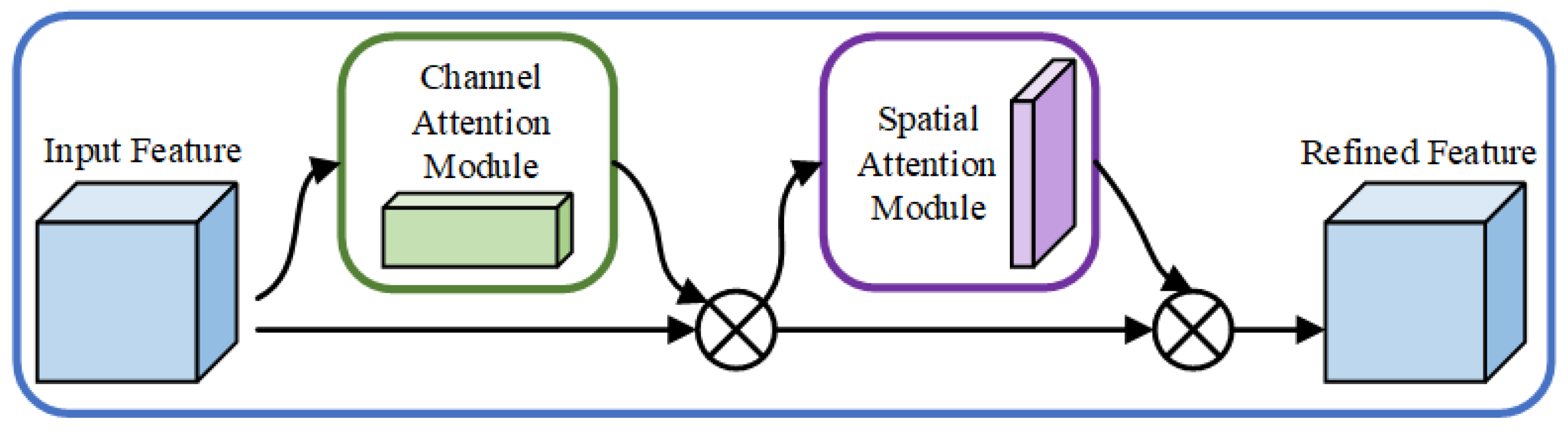
The Convolutional Attention Module (CBAM) is mainly composed of two parts, including the channel attention mechanism and the spatial attention mechanism, and its overall framework is shown in Figure 4. The attention module pays attention to the correlation between different channels and obtains the weights of different channels by calculation, which will be applied to the extracted channels to learn the characteristics of different channels. The role of the spatial attention module is to capture the spatial correlation between different pixel locations in the feature map, since pixels at different locations are of differing importance for the network to learn.
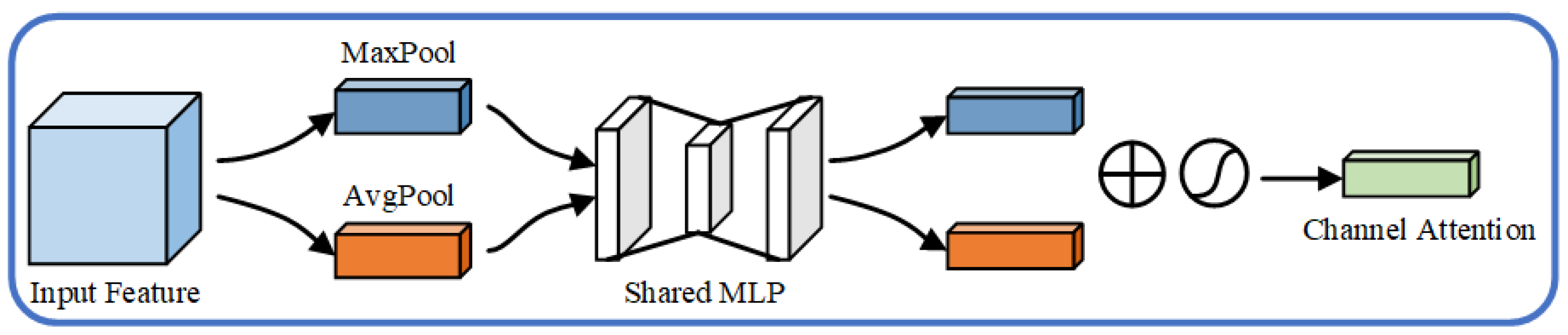
The structure of the channel attention module is shown in Figure 5. It reduces the dimension of the input features and performs max pooling and average pooling, respectively. Then, two 1 × 1 × C feature vectors are obtained, both of which contain the global distribution of the input features in the channel dimension. At the same time, in order to reduce the amount of calculation, a convolution is adopted to reduce the dimension of the two feature vectors, so that the numbers of channels are reduced to 1   /   16 of the previous. Meanwhile, the two reduced feature vectors are superimposed, which are fused by a 1 × 1 convolution, and the numbers of channels are restored to the original number C. Finally, through a sigmoid function, the channel attention matrix C A c k is obtained. The matrix is multiplied by the input elements to realize the adaptive adjustments of the original input characteristics in the channel dimension. The calculation process of the channel attention module [21] is shown in Formula (9):
M c h a n n e l = C A c h · f c h = σ ( δ ( w 1 · ( w 0 · v m a x + w 0 · v a v g ) ) ) · f c h
where σ represents the sigmoid function, W 0 R C / r × C and W 1 R C × C / r , which, respectively, represent the weights of the two 1 × 1 convolution kernels. Meanwhile, the δ ( · ) represents the RuLU activation function, and the v m a x and v a v g , respectively, represent the feature vectors after max pooling and average pooling.
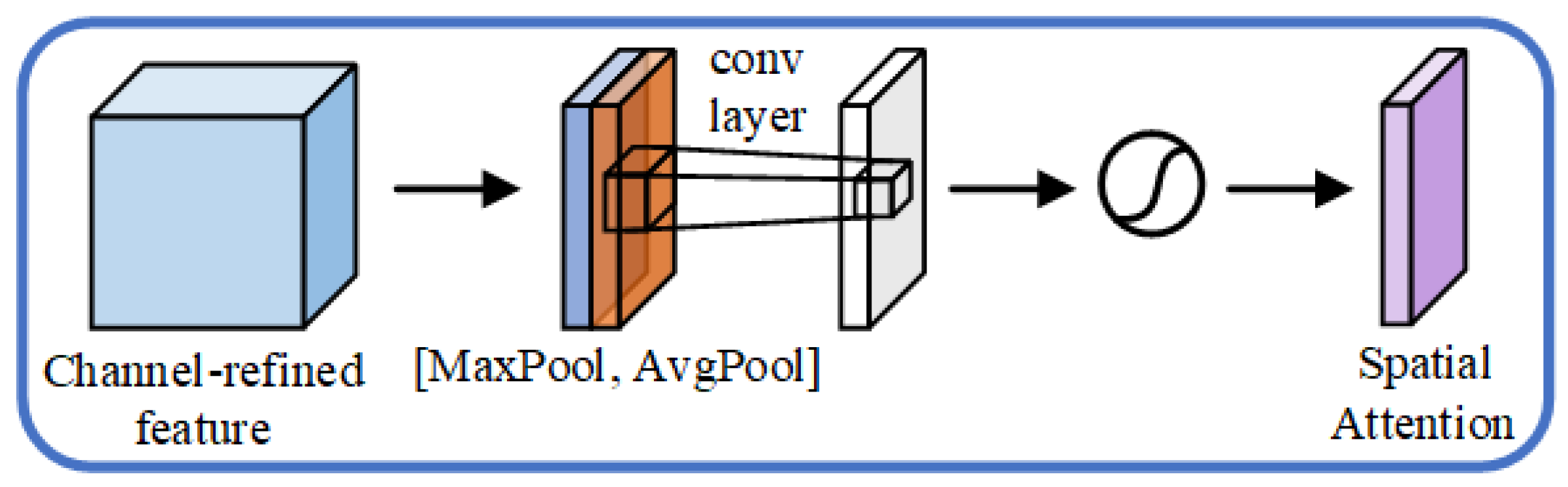
The process of the spatial attention module is similar to that of the channel attention module. The structure is shown in Figure 6. Firstly, the max-pooling and average-pooling operations are performed on the features extracted by channel attention along the channel, respectively, and the input feature maps of H × W × C are compressed into two single-channel feature maps of H × W × 1 , which shows the distribution of the input over the spatial dimension. Secondly, two single-channel feature maps are spliced in the channel dimension, and then fused using the convolution operation to obtain a feature map of H × W × 1 . Then, the spatial attention matrix S A c h is achieved through a sigmoid function. The matrix is multiplied by the elements of the original input features, resulting in a feature representation refined by two attentions. The calculation process of the spatial attention module is shown in Formula (10):
F s p a t i a l = S A c h · f c h a n n e l = σ ( δ ( w 2 · ( f m a x + f a v g ) ) ) · f c h a n n e l
where F s p a t i a l represents the feature extracted by the attention module, and w 2 represents the weights of the 1 × 1 convolution kernel. Two different feature descriptions f m a x and f a v g , respectively, represent the feature map after max pooling and average pooling.

2.2.3. Deep and Cross Fusion Method

After obtaining the 2D and 3D time-series characteristics of tropical cyclones, it is necessary to fuse the two features. In this paper, Deep and Cross Network (DCN) [22] is adopted to solve the problem of CTR estimation for large-scale sparse features. This model is a follow-up study of the Wide and Deep [
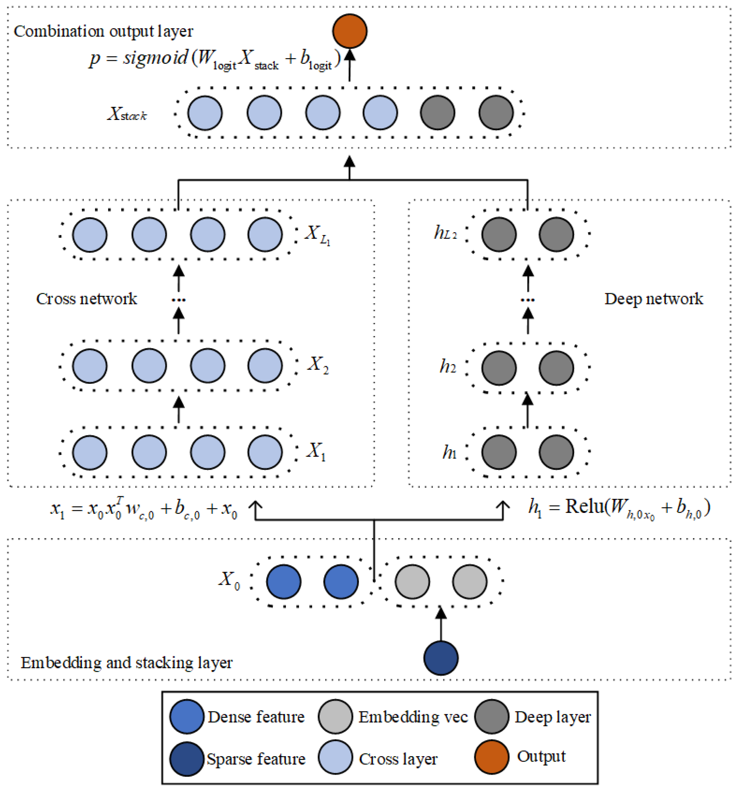
23] model, which replaces the wide part with the cross part implemented by a special network structure. The DCN can automatically construct limited high-order cross-features and learn the corresponding weights in the case of sparse and dense inputs, without manual feature engineering or exhaustive searching. The structure of Deep and Cross is shown in Figure 7.
A DCN model starts with an embedding and stacking layer, followed by a cross network and a deep network in parallel. These are followed by a combination layer which combines the outputs from the two networks.
We take the 2D features of tropical cyclones as dense features (light blue circles in Figure 7) and 3D features as sparse features (dark blue circles in Figure 7). After embedding, they are transformed into low-dimensional dense features. The embedding operation [22] is shown in Formula (11).
x e m b e d ,   i = W e m b e d ,   i x i
where x e m b e d ,   i is the embedding vector of the l t h category feature, corresponding to the 3D features after the embedding operation, and W e m b e d ,   i is the embedding matrix. Finally, this layer needs to combine dense features with the 3D features transformed by embedding, and then the vector is shown in Formula (12).
x 0 = [ x e m b e d , 1 T , , x e m b e d , k T , x d e n s e T ]
where the vector x 0 represents the combination of the 2D and 3D features of the tropical cyclones.
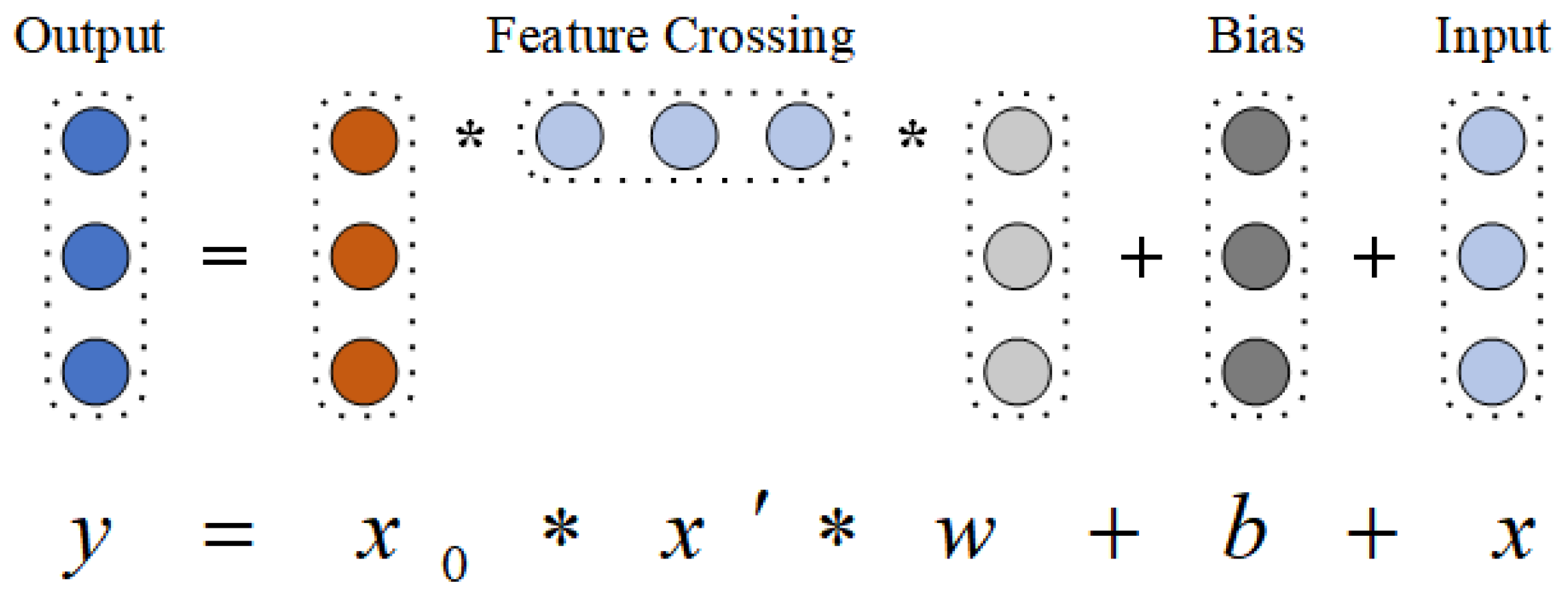
For the cross network, the purpose of the network is to increase the interaction between different features. The cross network is represented by multiple cross layers. Assuming that the output vector of the l t h layer is x 0 , then for the l + 1 t h layer, the output vector is x l + 1 , as shown in Formula (13).
x l + 1 = x 0 x l T w l + b l + x l = f ( x l , w l , b l ) + x l
where w l and b l are the weight and bias of the l t h layer. After each intersection layer completes the feature intersection, it will add the original input of the layer. The visualization of a cross layer is shown in Figure 8.
Each layer adds an n-dimensional weight vector w l , where n represents the dimension of the input vector, and the input vector is retained at each layer. Finally, after the 2D time series characteristics of tropical cyclones are operated by the cross network, a 2D model of tropical cyclones with memory has been established.
For the deep network, the network is a fully connected feedforward neural network, and each deep layer has the following formula:
h l + 1 = f ( W l h l + b l )
where h l , h l + 1 are the l t h and ( l + 1 ) t h hidden layer, respectively. W l , b l are parameters for the l t h deep layer, and f ( · ) is the RuLU function.
We take the 3D time series features of tropical cyclones based on the CBAM and multi-ConvGRU as deep part, which builds a generalized 3D model of tropical cyclones through deep learning and can be used to extract the deep features of tropical cyclones.
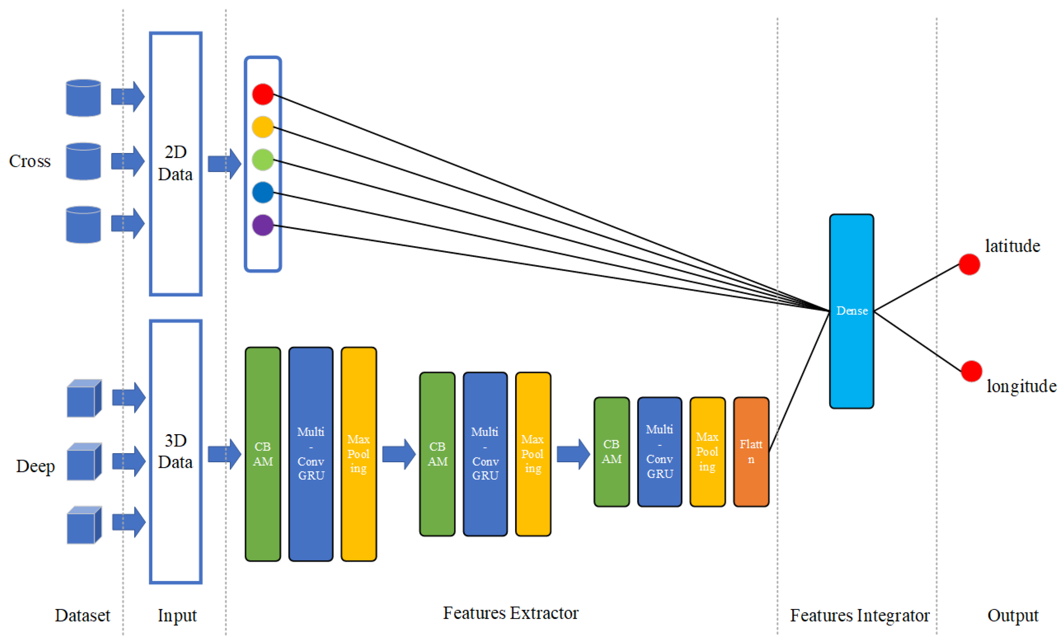
Since we adopt two dimensions of tropical cyclone data, after fusing the 2D and 3D features, we also add a neural network as the fusion network of the two features. The structure of the network is shown in Figure 9.
For the cross part, the 2D time series structure of tropical cyclones is constructed according to the CMA dataset, and CNN is adopted as the cross-part model. For the deep part, the 3D time series structure of the tropical cyclones and its surroundings are constructed according to the geopotential variables. Then, we use three network layers including the CBAM layer, multi-ConvGRU layer, and max pooling layer as a stacking block. Thereafter, the stacked layers are repeated three times, where the first two times are processed on multiple time dimensions, whereas the last time is processed in the current time dimension. The network finally flattens all the features and obtains the features of the cross part and the deep part. We jointly train the two parts and add a layer of neural network to integrate the features of the two parts. Finally, the network forecasts the central latitude and longitude of a tropical cyclone for the next 24 h.
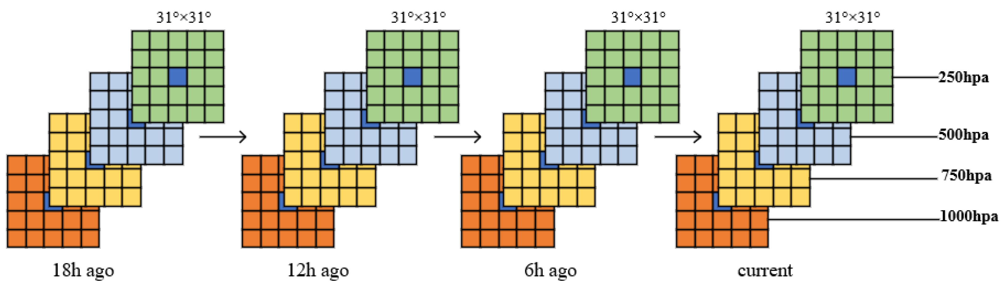
According to the pre-processing of 3D data in Chapter 3, we obtain the 3D time series structure of a tropical cyclone. Since the batch size of data has been set to 128, the shape of the input data is (128, 4, 4, 31, 31), which means (batch, timesteps, channels, height, width). After the input data operated by the three stacking blocks and FC, the shape of the output data is (128, 128). The process of data flow is shown in Table 2. At the same time, we obtain the 2D typhoon data processed by CLIPER, the shape of which is (128, 53). Then, we combine the cross and deep features in a dense layer, whose shape is (128, 128 + 53). After two Full Connection Layers, the shape of the output data is (128, 2), which represents the forecasting latitude and longitude of each batch. We obtain the latitude and longitude of the tropical cyclone in the next 24 h.

3. Results

3.1. Experimental Designs

This chapter designs four experiments to verify the performance of our model. The first one tests the effectiveness of CNN, whose purpose is to analyse whether CNN can more effectively characterize the 2D features of tropical cyclones. The second experiment evaluates whether the CBAM and multi-ConvGRU methods can improve forecasting accuracy based on the Deep and Cross framework. The third experiment compares the proposed method with the traditional tropical cyclone forecasting method and evaluates whether the proposed model has advantages compared with the traditional model. The fifth experiment evaluates the performance of the proposed method in long-term forecasting.

3.1.1. Datasets Pre-Processing

For the experiments, the CMA and EAR-Interim datasets were aligned through the temporal and spatial domains. Then, the datasets were divided into three parts, including training set, validation set, and testing set. The training set selected tropical cyclones data recorded from 2000 to 2016. For the validation set, 10% of the training set was chosen randomly. For the testing set, tropical cyclones recorded from 2017 to 2020 were selected. The experimental data are shown in Table 3.
For the CMA dataset, we ignored tropical cyclones with fewer than 14 records because the duration of such tropical cyclones was so short that we could not establish the CLIPER method. In addition, the training set, validation set, and test set are normalized by the Min-Max method.
The 36 historical records of tropical cyclone “Cuckoo” are shown in Table 4, including the longitude, latitude, timestamp, and meteorological attributes of the tropical cyclone landing.

3.1.2. Experimental Environment

The experiments were performed on a computer equipped with an Intel® Xeon® Gold 6230 CPU® 2.10 Ghz sourced by Intel, Santa Clara, CA, USA, a RTX A6000 GPU sourced by Nvidia, Santa Clara, CA, USA and 128GB RAM sourced by Kingston, Fountain Valley, CA, USA. We adopted the PyTorch deep learning framework to build the model and conduct our experiments.

3.1.3. Evaluation Criteria

In order to evaluate the track forecasting results, we used the Great Circle Distance, a common metrics tool to measure the error distance between model forecasting and ground truth. The Great Circle Distance can be computed by:
D = 2 × R × q u a d   arcsin ( sin 2 ( | X p X r | 2 ) + cos X P cos X r sin 2 ( | β p β r | 2 ) )
where R 6371   km represents the radius of Earth; X r and β r stand for the latitude and longitude of ground truth. X P and β p indicate the latitude and longitude of the forecasting.

3.2. Evaluating Cross Part’s Effectiveness

This experiment intended to evaluate whether CNN performed well for the cross part. CNN was compared with several existing machine learning methods, such as SVM [6], GBDT [18], LSTM [24], GRU [25], RNN [9], and 1D CNN [13]. The experimental results are shown in Table 5.
The experiment in Table 5 shows the annual forecasting error (km) of each comparison method, as well as the average error of all years. Compared with the machine learning methods based on a decision tree (SVM and GBDT), the accuracy of the 1D CNN was improved by 3.46~6.65%. Because 2D tropical cyclones are a combination of linear and nonlinear attributes, these models have a limited ability to model 2D tropical cyclones. Afterwards, we compared 1D CNN with deep learning methods (LSTM, GRU and RNN), and the 1D CNN obtained a 5.97~14.99% improvement in distance error. There are two possible reasons that explain why the deep learning methods achieve poor performances. Firstly, the amount of data for 2D tropical cyclones is too small. Secondly, there are only four available features (latitude, longitude, wind speed, and pressure) in the CMA dataset. Overall, the 1D CNN worked better as a cross component to forecast the 24-h tracks of tropical cyclones.

3.3. Evaluating the Deep and Cross Framework’s Effectiveness

In order to evaluate whether the fused atmospheric reanalysis data can improve the forecasting accuracy, in the deep part, we used 2D CNN [14], ConvLSTM [11], ConvGRU [26], multi-ConvGRU, and multi-ConvGRU + CBAM to conduct comparative experiments. Furthermore, we tested the proposed method and compared methods using different numbers of isobars, which were one isobaric plane (500 hPa); four isobaric planes (1000 hPa, 750 hPa, 500 hPa and 250 hPa); and eight isobaric planes (1000 hPa, 900 hPa, 800 hPa, 700 hPa, 600 hPa, 500 hPa, 400 hPa, 300 hPa). We selected the current time for a single time step, and selected the current time, the previous 6 h, the previous 12 h, and the previous 18 h for multiple time steps.
We applied the 1D CNN to the cross part and 2D CNN to the deep part, and under a single isobaric surface, we conducted comparative experiments using single and multiple time steps. The experimental results are shown in Table 6. The forecasting accuracy of using 2D CNN to extract the 3D features of tropical cyclones and fusing them with the 2D features was about 22.96% higher than that of using only 2D features, the reasons for which are that the characteristics of multiple dimensions can help the deep learning models to learn the laws of movements of tropical cyclones more effectively. Meanwhile, under the conditions of the 2D and 3D features of tropical cyclones, the forecasting accuracy with multiple time steps was improved by about 6.92%, compared to using a single time step. We concluded that the forecasting accuracy can be improved by combining the 3D model of tropical cyclones at different times in the past.
The experimental results in Table 7 present the distance error to evaluate the 24-h forecasting accuracy of different methods under four isobaric surfaces. For the cross part with 1D CNN and the deep part with 2D CNN, whether it was a single or multiple time step, the forecasting accuracy under four isobaric surfaces was 1.12~2.73% higher than that of a single isobaric surface. This is because the deep learning model has better spatial feature extraction abilities. Moreover, under the multi-time-step condition where 1D CNN was adopted in the cross part, the ConvGRU obtained about 3.75% improvement over the ConvLSTM. As the parameters of ConvLSTM are too many, it is easy to cause overfitting of the model. Since the multi-convolution module can extract wider and deeper spatial nonlinear features, the multi-ConvGRU performed better than ConvGRU, which was improved by about 1.85~4.20%. Meanwhile, we applied the CBAM mechanism to the multi-ConvGRU. The experimental results show that the multi-convolution model adopting the attention mechanism performed better than other methods, whose forecasting accuracy was improved about 2.40~32.86%. The reason is that the large-scale problem of a high-response isobaric surface affecting the tropical cyclone can be overcome by the CBAM.
Table 8 shows the distance error to evaluate the 24-h forecasting results of different methods under eight isobaric surfaces. Under the single and multiple time steps, for the cross part with 1D CNN and the deep part with 2D CNN, the forecasting accuracy under eight isobaric surfaces was slightly higher than that under four isobaric surfaces, since CNN had a strong ability to extract spatial features. However, under the condition that ConvLSTM and ConvGRU are adopted in the deep part in multiple time steps, compared with four isobaric surfaces, the forecasting accuracy under eight isobaric surfaces decreased by 3.27~8.00%, which showed that the forecasting accuracy reduced while the number of isobaric surfaces increased. When the isobaric surfaces increase to a certain number, the ability of ConvLSTM and ConvGRU to extract the 3D features of tropical cyclones is limited. Thanks to the powerful spatial feature extraction ability of the multi-convolution module, multi-ConvGRU improved about 2.09% more than ConvGRU in forecasting accuracy. Overall, after adding the CBAM mechanism, the multi-ConvGRU model performed better than other models. It can be proved that the attention mechanism can indeed improve the forecasting accuracy of tropical cyclones.
In order to show whether the experimental results have statistical significance in Table 5, Table 6, Table 7 and Table 8, we conducted significance testing. Significance testing [27,28] is a term used to describe whether the differences between the results of the experimental group and control group are significant, rather than due to chance. Since each table contained more than two forecasting results, we adopted ANOVA (analysis of variance) [29] to conduct the significance of each table, as shown in Table 9. After performing the ANOVA, the statistic and p-value were obtained. The p-value is a target to measure the differences between the results of the experimental group and control group. For the statistical significance, value α represents the significance level and is generally set to 0.05 [29]. If the p-value is above α , the table’s results are not statistically significant, and if it is below α , then the opposite is true. According to the testing, in addition to Table 5, the p-values of Table 6, Table 7 and Table 8 are less than 0.05, and the statistics of these three tables are larger, indicating that the results in Table 6, Table 7 and Table 8 are significantly different.

3.4. Comparison with Traditional and Deep Learning Methods

In this section, we compare the proposed method with traditional and deep learning methods for tropical cyclone forecasting. We selected CLIPER [18] as the traditional method for comparison. This method uses correlation analysis to screen climate persistence factors and build a multiple linear regression model, which can be treated as the baseline of other forecasting methods. Meanwhile, we selected LSTM, GRU [25], NMPT [30], GBRNN [9], and CMO [31] as deep learning methods. NMPT is a model based on the LSTM network model, and GBRNN is a variant of RNN that uses network boundaries to finish the tropical cyclone forecasting. The Central Meteorological Observatory (CMO) adopts the numerical prediction method to forecast tropical cyclone paths, which is a traditional tropical cyclone forecasting method [32]. These models were adopted to forecast the tracks of tropical cyclones in the next 6 h, 12 h and 24 h.
As shown in Table 10, compared with the benchmark model CLIPER, the distance error of the proposed method is less than that of the CLIPER method, which demonstrates the practical availability of our model. Compared with the deep learning methods such as NMPT and GBRNN, the forecasting accuracy of our method was 17.3~44.9% higher than that of NMPT, and 5.20~5.40% higher than that of GBRNN. Then, our method improved by 20.04~50.2% in forecasting accuracy, compared to the LSTM and GRU. Our model performed better than the traditional and deep learning methods in the 24-h tropical cyclone forecasting. Finally, we compared the proposed model to the CMO’s method. Our model had a 1.8% improvement in track forecasting in 6 h but performed worse than that of the CMO in 12 h and 24 h.

3.5. Evaluating the Long-Term Foresting Ability

In order to evaluate the performance of the proposed model for long-term forecasting, we compared the distance error of tropical cyclones forecasting with our model and CMO’s approach in 6 h, 12 h, 24 h, 48 h and 72 h. The experimental results are shown in Table 11.
Our proposed model only performed better in the 6-h forecasting, Meanwhile, the gap in forecasting accuracy between our model and CMO’s method widened with time. Our model is limited in long-term tropical cyclone track forecasting. This also means that the features extracted by our proposed model from the used historical data do not support long-term tropical cyclone forecasting,

3.6. Visualization of Forecasting Results

In order to show the actual forecasting accuracy of our model, we have visualized the tropical cyclones Yutu and Nasa, which occurred in 2018 and 2017. Figure 10 and Figure 11 show the 24-h forecasting paths of the two tropical cyclones, respectively. We use the tropical cyclone paths forecasted by the CNN in the cross part as the baseline path. Meanwhile, the real path adopts the tropical cyclone information from the CMA dataset. Overall, it is observed that the proposed method outperforms the baseline method in terms of distance error.

4. Conclusions

This paper proposes a neural network model for tropical cyclone track forecasting based on attention mechanism and multi-ConvGRU. For the large-scale problem of high response isobaric surface, this model adopts the Convolutional Block Attention Mechanism (CBAM), which considers isobaric planes at different altitudes to establish the 3D structure of tropical cyclones. Moreover, this paper proposes multi-ConvGRU to extract the large-scale nonlinear spatial features of tropical cyclones. In addition, the Deep and Cross framework is adopted to fuse the 2D and 3D features of tropical cyclones, where CNN processes the 2D features and multi-ConvGRU handles the 3D features.
The experiments were conducted on the CMA Tropical Cyclone Best Track dataset and EAR-Interim reanalysis atmospheric data to demonstrate the effectiveness of the proposed model. The results show that the track forecasting model that fuses the 2D and 3D features of tropical cyclones provides a more significant improvement than the model using a single feature. In addition, our model is superior to deep learning tropical cyclone forecasting methods.
Although the deep learning method combined with the CLIPER method has greatly improved, it still has a large gap compared with the current dynamic method. At the same time, statistical forecasting methods have limited consideration of special situations other than tropical cyclones. It may be necessary to introduce tropical cyclone travel rules in the future to strengthen the forecasting accuracy.

Author Contributions

Conceptualization, W.F. and W.L.; methodology, W.F.; software, W.F.; validation, W.L.; formal analysis, W.F.; investigation, W.L.; resources, J.L.; data curation, W.F.; writing—original draft preparation, W.F.; writing—review and editing, W.L. and L.Z.; visualization, J.L.; supervision, W.L.; project administration, W.L. and J.L.; funding acquisition, W.L. All authors have read and agreed to the published version of the manuscript.

Funding

This research was funded by the National Natural Science Foundation of China (Grant No. 42075007), the Open Grants of the State Key Laboratory of Severe Weather (No. 2021LASW-B19).

Institutional Review Board Statement

Not applicable.

Informed Consent Statement

Not applicable.

Data Availability Statement

CMA Tropical Cyclone Best Track Dataset are available at https://tcdata.typhoon.org.cn/en/zjljsjj_sm.html (accessed on 1 May 2022); ERA-Interim data are available at https://apps.ecmwf.int/datasets/data/interim-full-daily/levtype=sfc/ (accessed on 1 May 2022).

Conflicts of Interest

The authors declare no conflict of interest.

References

  1. Neumann, C.J. An alternate to the HURRAN (Hurricane Analog) Tropical Cyclone Forecast System. 1972. Available online: https://repository.library.noaa.gov/view/noaa/3605 (accessed on 1 April 2022).
  2. Knaff, J.A.; Sampson, C.R.; Musgrave, K.D. Statistical tropical cyclone wind radii prediction using climatology and persistence: Updates for the western North Pacific. Weather. Forecast. 2018, 33, 1093–1098. [Google Scholar] [CrossRef]
  3. Geoghegan, K.M.; Fitzpatrick, P.; Kolar, R.L.; Dresback, K.M. Evaluation of a synthetic rainfall model, P-CLIPER, for use in coastal flood modeling. Nat. Hazards 2018, 92, 699–726. [Google Scholar] [CrossRef]
  4. Hsan, T.Z.; Sein, M.M. Combining Support Vector Machine and Polynomial Regressing to Predict Tropical Cyclone Track. In Proceedings of the 2021 IEEE 3rd Global Conference on Life Sciences and Technologies (LifeTech), Nara, Japan, 9–11 March 2021; pp. 220–221. [Google Scholar]
  5. Chen, P.H.; Lin, C.J.; Schölkopf, B. A tutorial on ν-support vector machines. Appl. Stoch. Models Bus. Ind. 2005, 21, 111–136. [Google Scholar] [CrossRef]
  6. Song, H.J.; Huh, S.H.; Kim, J.H.; Ho, C.H.; Park, S.K. Typhoon track prediction by a support vector machine using data reduction methods. In Proceedings of the International Conference on Computational and Information Science, Berlin, Germany, 9–12 May 2005; pp. 503–511. [Google Scholar]
  7. Rüttgers, M.; Lee, S.; Jeon, S.; You, D. Prediction of a typhoon track using a generative adversarial network and satellite images. Sci. Rep. 2019, 9, 6057. [Google Scholar] [CrossRef] [PubMed]
  8. Goodfellow, I.; Pouget-Abadie, J.; Mirza, M.; Xu, B.; Warde-Farley, D.; Ozair, S.; Courville, A.; Bengio, Y. Generative adversarial nets. Adv. Neural Inf. Process. Syst. 2014, 27, 139–144. [Google Scholar]
  9. Alemany, S.; Beltran, J.; Perez, A.; Ganzfried, S. Predicting hurricane trajectories using a recurrent neural network. In Proceedings of the AAAI Conference on Artificial Intelligence, Honolulu, HA, USA, 1–27 January 2019; pp. 468–475. [Google Scholar]
  10. Hochreiter, S.; Schmidhuber, J. Long short-term memory. Neural Comput. 1997, 9, 1735–1780. [Google Scholar] [CrossRef]
  11. Kim, S.; Kim, H.; Lee, J.; Yoon, S.; Kahou, S.E.; Kashinath, K.; Prabhat, M. Deep-hurricane-tracker: Tracking and forecasting extreme climate events. In Proceedings of the 2019 IEEE Winter Conference on Applications of Computer Vision (WACV), Waikoloa Village, HA, USA, 7–11 January 2019; pp. 1761–1769. [Google Scholar]
  12. Shi, X.; Chen, Z.; Wang, H.; Yeung, D.Y.; Wong, W.K.; Woo, W.C. Convolutional LSTM network: A machine learning approach for precipitation nowcasting. Adv. Neural Inf. Process. Syst. 2015, 28, 802–810. [Google Scholar]
  13. Giffard-Roisin, S.; Yang, M.; Charpiat, G.; Kumler, B.C.; Kégl, B.; Monteleoni, C. Tropical cyclone track forecasting using fused deep learning from aligned reanalysis data. Front. Big Data 2020, 3, 1. [Google Scholar] [CrossRef]
  14. Chen, R.; Wang, X.; Zhang, W.; Zhu, X.; Li, A.; Yang, C. A hybrid CNN-LSTM model for typhoon formation forecasting. GeoInformatica 2019, 23, 375–396. [Google Scholar] [CrossRef]
  15. Ying, M.; Zhang, W.; Yu, H.; Lu, X.; Feng, J.; Fan, Y.; Fan, Y.; Zhu, Y.; Chen, D. An overview of the China Meteorological Administration tropical cyclone database. J. Atmos. Ocean. Technol. 2014, 31, 287–301. [Google Scholar] [CrossRef]
  16. Lu, X.; Yu, H.; Ying, M.; Zhao, B.; Zhang, S.; Lin, L.; Bai, L.; Wan, B. Western North Pacific tropical cyclone database created by the China Meteorological Administration. Adv. Atmos. Sci. 2021, 38, 690–699. [Google Scholar] [CrossRef]
  17. Dee, D.P.; Uppala, S.M.; Simmons, A.J. The ERA-Interim reanalysis: Configuration and performance of the data assimilation system. Q. J. R. Meteorol. Soc. 2011, 137, 553–597. [Google Scholar] [CrossRef]
  18. Tan, J.; Chen, S.; Wang, J. Western North Pacific tropical cyclone track forecasts by a machine learning model. Stoch. Environ. Res. Risk Assess. 2021, 35, 1113–1126. [Google Scholar] [CrossRef]
  19. Xu, G.; Xian, D.; Fournier-Viger, P.; Li, X.T.; Ye, Y.M.; Hu, X.Q. AM-ConvGRU: A spatio-temporal model for typhoon path prediction. Neural Comput. Appl. 2022, 34, 5905–5921. [Google Scholar] [CrossRef]
  20. Shi, X.; Gao, Z.; Lausen, L. Deep learning for precipitation nowcasting: A benchmark and a new model. Adv. Neural Inf. Process. Syst. 2017, 30, 5617–5627. [Google Scholar]
  21. Woo, S.; Park, J.; Lee, J.Y.; Kweon, I.S. Cbam: Convolutional block attention module. In Proceedings of the European Conference on Computer Vision (ECCV), Munich, Germany, 8–14 September 2018; pp. 3–19. [Google Scholar]
  22. Wang, R.; Fu, B.; Fu, G.; Wang, M. Deep & cross network for ad click predictions. In Proceedings of the ADKDD’17, Halifax, NS, Canada, 14 August 2017; pp. 1–7. [Google Scholar]
  23. Cheng, H.T.; Koc, L.; Harmsen, J. Wide & deep learning for recommender systems. In Proceedings of the 1st Workshop on Deep Learning for Recommender Systems, Boston, MA, USA, 15 September 2016; pp. 7–10. [Google Scholar]
  24. Kumar, S.; Biswas, K.; Pandey, A.K. Track Prediction of Tropical Cyclones Using Long Short-Term Memory Network. In Proceedings of the 2021 IEEE 11th Annual Computing and Communication Workshop and Conference (CCWC), Las Vegas, NV, USA, 27–30 January 2021; pp. 0251–0257. [Google Scholar]
  25. Dong, P.; Lian, J.; Zhang, Y. A novel data-driven approach for tropical cyclone tracks prediction based on Granger causality and GRU. In Proceedings of the 2019 IEEE International Conference on Service Operations and Logistics, and Informatics (SOLI), Zhengzhou, China, 6–8 November 2019; pp. 70–75. [Google Scholar]
  26. Zhang, Z.; Yang, X.; Shi, L.; Wang, B.; Du, Z.; Zhang, F.; Liu, R. A neural network framework for fine-grained tropical cyclone intensity prediction. Knowl.-Based Syst. 2022, 241, 108195. [Google Scholar] [CrossRef]
  27. Sirkin, R.M. Statistics for the Social Sciences, 3rd ed.; SAGE Publications: Thousand Oaks, CA, USA, 2005; pp. 271–316. [Google Scholar]
  28. Borror, C.M. The Certified Quality Engineer Handbook, 3rd ed.; ASQ Quality Press: Milwaukee, WI, USA, 2009; pp. 418–472. [Google Scholar]
  29. St, L.; Wold, S. Analysis of variance (ANOVA). Chemom. Intell. Lab. Syst. 1989, 6, 259–272. [Google Scholar]
  30. Gao, S.; Zhao, P.; Pan, B.; Li, Y.; Zhou, M.; Xu, J.; Zhong, S.; Shi, Z. A nowcasting model for the prediction of typhoon tracks based on a long short term memory neural network. Acta Oceanol. Sin. 2018, 37, 8–12. [Google Scholar] [CrossRef]
  31. CMO. Typhoon Network of Central Meteorological Observatory. 2019. Available online: http://typhoon.nmc.cn/web.html (accessed on 1 May 2022).
  32. Li, Z.; Zhang, L.; Qian, Q.; Ma, S.; Xu, J.; Dai, K.; Chen, Y.; Wang, Y. The development and consideration of typhoon forecast operation of national Meteorological Center. Trans. Atmos. Sci. 2020, 43, 10–19. [Google Scholar]
Figure 1. The visualization of the CMA dataset’s tropical cyclone paths.
Atmosphere 13 01607 g001
Figure 2. The 2D structure of each isobaric surface of a tropical cyclone, reprinted with permission from Ref. [19]. 2022, Springer Nature.
Atmosphere 13 01607 g002
Figure 3. The 3D time series structure of a tropical cyclone, reprinted with permission from Ref. [19]. 2022, Springer Nature.
Atmosphere 13 01607 g003
Figure 4. The structure of CBAM, reprinted with permission from Ref. [21]. 2018, Spring Nature.
Atmosphere 13 01607 g004
Figure 5. The structure of the channel attention module, reprinted with permission from Ref. [21]. 2018, Springer Nature.
Atmosphere 13 01607 g005
Figure 6. The structure of the spatial attention module, reprinted with permission from Ref. [21]. 2018, Springer Nature.
Atmosphere 13 01607 g006
Figure 7. The structure of Deep and Cross [22].
Atmosphere 13 01607 g007
Figure 8. The visualization of a cross layer [22].
Atmosphere 13 01607 g008
Figure 9. The structure of the tropical cyclone forecasting model.
Atmosphere 13 01607 g009
Figure 10. Visualization of 24-h path forecasting of tropical cyclone Yutu.
Atmosphere 13 01607 g010
Figure 11. Visualization of 24-h path forecasting of tropical cyclone Nasha.
Atmosphere 13 01607 g011
Table 1. Two-Dimensional Characteristics of Tropical Cyclone Tracks.
IDFeature NameDescription
X1–X5LAT0, LAT6, LAT12, LAT18, LAT24Past 6-h, 12-h, 18-h, 24-h latitude
X6–X10LONG0, LONG6, LONG12, LONG18, LONG24Past 6-h, 12-h, 18-h, 24-h longitude
X11–X15WND0, WND6, WND12, WND18, WND24Past 6-h, 12-h, 18-h, 24-h wind speed
X16MonthCurrent month
X17–X18LAT0–LAT6, LAT6–LAT12Past 6 h–12 h first-order difference in historical latitude
X19–X20LAT12–LAT18, LAT18–LAT24Past 12 h–24 h first-order difference in historical latitude
X21–X22LONG0–LONG6, LONG6–LONG12Past 6 h–12 h first-order difference in historical longitude
X23–X24LONG12–LONG18, LONG18–LONG24Past 12 h–24 h first-order difference in historical longitude
X25–X26WND0-WND6, WND6-WND12Past 6 h–12 h first-order difference in historical wind speed
X27–X28WND12-WND18, WND18-WND24Past 12 h–24 h first-order difference in historical wind speed
X29 i = 0 3 ( LAT 6 i LAT 6 ( i + 1 ) ) 2 Sum of squares of X17–X20
X30 i = 0 3 ( LONG 6 i LAT 6 ( i + 1 ) ) 2 Sum of squares of X21–X24
X31 i = 0 3 ( LAT 6 i LAT 6 ( i + 1 ) ) 2 Square root of feature X29
X32 i = 0 3 ( LONG 6 i LAT 6 ( i + 1 ) ) 2 Square root of feature X30
X33–X34 LAT ,   LONG Square root of current latitude and longitude
X35–X36ACC(LOC0, LOC6), ACC(LOC6, LOC12)Past 6 h–12 h physical acceleration
X37–X38ACC(LOC12, LOC18), ACC(LOC18, LOC24)Past 12 h–24 h physical acceleration
X39–X40Angle(LAT0 ,   0 ° N ) ,   Angle ( LAT 6 ,   0 ° N)Past 6 h angle between position and latitude
X41–X42 Angle ( LAT 12 ,   0 ° N ) ,   Angle ( LAT 18 ,   0 ° N)Past 18 h angle between position and latitude
X43–X44Angle(LOC0 ,   0 ° E ) ,   Angle ( LOC 6 ,   0 ° E)Past 6 h angle between position and longitude
X45–X46 Angle ( LOC 12 ,   0 ° E ) ,   Angle ( LOC 18 ,   0 ° E)Past 18 h angle between position and longitude
X47Angle(PATH0,6, PATH6,12)Past 6 h–12 h angle of path
X48Angle(PATH6,12, PATH12,18)Past 12 h–18 h angle of path
X49Angle(PATH12,18, PATH18,24)Past 18 h–24 h angle of path
X50–X51Angle(LOC, LOC6), Angle(LOC6, LOC12)Past 6 h–12 h angle of heading
X52–X53Angle(LOC12, LOC18), Angle(LOC18, LOC24)Past 12 h–24 h angle of heading
Table 2. The specific model parameters of the Deep model.
Layer NameModelIn/OutOutput Size
Block1CBAM4/64(128, 4, 4, 31, 31)
multi-ConvGRU(128, 4, 64, 31, 31)
MaxPooling(128, 4, 64, 15, 15)
Block2CBAM64/128(128, 4, 64, 15, 15)
multi-ConvGRU(128, 4, 128, 15, 15)
MaxPooling(128, 4, 128, 7, 7)
Block3CBAM128/256(128, 4, 128, 7, 7)
multi-ConvGRU(128, 256, 7, 7)
MaxPooling(128, 256, 3, 3)
FCFlatten (256*3*3, 128)
Table 3. Partition of the experimental dataset.
ParametersValue
Datasets amount12,318 records
Training set9803 tuples
Testing set2515 tuples
Validation set980 tuples
Temporal dimension24-h
Table 4. Data representation of tropical cyclone Cuckoo.
TIDYEARMONTHDAYHOURLATLONGWNDPRESNAME
225520159241218.7132.425990Dujuan
225520159241818.9132.228985Dujuan
22552015925019.2132.030980Dujuan
225520159256195131.733975Dujuan
2255201592512198131.335970Dujuan
225520159296255117.620995Dujuan
2255201592912264116.4151000Dujuan
2255201592918274115.9101006Dujuan
225520159300280116.3101008Dujuan
225520159306287116.6101010Dujuan
Table 5. Twenty-four hour distance error in cross component (km).
2017201820192020AVG
SVM182.12224.82244.63250.46225.51
GBDT180.43215.38232.75237.85216.60
LSTM184.24230.67245.95228.63222.37
GRU183.89225.58237.43228.78218.92
RNN202.57248.46265.73267.18245.98
1D CNN173.31219.18226.39217.53209.10
Table 6. Twenty-four hour distance error of single isobaric surface forecast (km).
2017201820192020AVG
1D CNN173.31219.18226.39217.53209.10
Single time step + 1D CNN + 2D CNN156.32149.27158.26180.57161.10
Multiple time step + 1D CNN + 2D CNN155.85140.87148.43154.64149.95
Table 7. Twenty-four hour distance error of four isobaric surfaces forecast (km).
2017201820192020AVG
1D CNN173.31219.18226.39217.53209.10
Single time step + 1D CNN + 2D CNN138.34163.23154.85172.45157.23
Multiple time step + 1D CNN + 2D CNN144.12146.75153.58154.06149.63
Multiple time step + 1D CNN + ConvLSTM140.84146.03155.71166.40152.25
Multiple time step + 1D CNN + ConGRU137.46139.10144.38165.21146.54
Multiple time step + 1D CNN+
multi-ConGRU
128.18146.69153.12147.32143.83
Multiple time step + 1D CNN+
multi-ConvGRU + CBAM
124.22145.69140.03151.58140.38
Table 8. Twenty-four hour distance error of eight isobaric surfaces forecast (km).
2017201820192020AVG
1D CNN173.31219.18226.39217.53209.10
Single time step + 1D CNN + 2D CNN143.84154.28161.87168.49157.12
Multiple time step + 1D CNN + 2D CNN136.43143.68152.38157.45147.49
Multiple time step + 1D CNN + ConvLSTM147.43153.84153.43174.21157.23
Multiple time step + 1D CNN + ConGRU148.49155.00154.32175.23158.26
Multiple time step + 1D CNN+
multi-ConGRU
148.89152.47151.59166.82154.94
Multiple time step + 1D CNN+
multi-ConvGRU + CBAM
133.22140.04152.24156.23145.43
Table 9. Statistical testing results in Table 5, Table 6, Table 7 and Table 8.
TableStatisticp-Value
Table 50.7218780.5903221
Table 614.5518470.0015127
Table 711.4598020.0000105
Table 810.6141490.0000188
Table 10. Six-, twelve-, and twenty-four-hour distance error of traditional and deep learning methods (km).
CLIPERLSTMGRUNMPTGBRNNCMOProposed
6 h201836.5445.2846.5644.1238.7537.3436.30
201937.2846.0645.7346.0037.3436.8035.76
202036.8643.5644.3642.0239.4637.2337.26
AVG36.8944.9745.5544.0538.5237.1236.44
12 h201871.43106.44106.56104.1869.7953.0366.85
201975.31104.68105.43105.4773.1251.0568.30
202070.5998.2699.0399.4474.2152.4270.03
AVG72.44103.13103.67103.0672.3752.1768.40
24 h2018161.75273.12274.76270.45152.2175.73140.04
2019165.18270.89271.14273.06162.4675.00152.24
2020160.69268.65269.54270.14158.3175.86156.24
AVG162.54270.89271.81271.22157.6775.53149.51
Table 11. Long-term distance error of CMO and proposed method (km).
6 h12 h24 h48 h72 h
CMO37.5654.1274.69135.02201.40
Proposed36.4468.40149.51340.14550.45
Publisher’s Note: MDPI stays neutral with regard to jurisdictional claims in published maps and institutional affiliations.

