The Space and Terrestrial Weather Variations as Possible Factors for Ischemia Events in Saint Petersburg

Abstract

The Space and Terrestrial Weather (Weather Complex) impact on ischemia cases in Saint Petersburg is investigated. The results show the main feature of the Weather Complex when it was related to the days of the different ischemia situations in the different ischemia people gender groups. The data treatment was done with some elements of the Folder Epochs Method, Cluster Analysis and the Mann–Whitney hypothesis test criterion.

1. Introduction

The study of a living organism sensitivity to environmental variations is an old subject. There is much information from the many researchers that have worked in this field in the past and work now.

A.L Tchijevsky, the Russian scientist, had investigated this subject in the first half of the 20th century [1,2,3,4]. He made more than a hundred works and claimed that the human organism senses all cosmic variations so space disturbances provoke human health problems. The scientific branch Geliobiology deals with this issue—the field of its study is the Space Weather impact on a living object. A continual line of these studies happened throughout the 20th century [5] and are successfully done now. Modern works in this field consider different aspects of such an impact. The significant part of these works carefully investigates the geomagnetic impact on the biosphere, which includes, of course, the human organism [6,7,8,9,10,11,12]. The information from the authors of the works mentioned above is important for the understanding of the mechanisms of the human body’s reaction to geomagnetic disturbances. The special consideration of the human heart function in the circumstance of magnetic instability [6,8,9,10,11] allows clarifying the heart’s response to geomagnetic storms. Additionally, there are interesting results of the psychological investigation [10,12] in the circumstances of the geomagnetic disturbances. Different works show the direction for the special investigation of the cosmic ray’s impact on the living organism; that impact is mediated by the ionosphere disturbances and the atmosphere electricity disturbances [7,13,14,15,16,17,18,19]. One should note the wide range of modern investigations—from the global impact of lunar phases [20] on the human organism to precise laboratory experiments of manmade physical fields (mostly electromagnetic field); those simulate natural physical fields and the impact of them on the different human organism points [18].

Much information we have from the investigations of Terrestrial Weather [20,21,22,23,24,25,26] is the field of the scientific branch Biometeorology. There are informative investigation results of the dependence of human health on air temperature anomalies [21,24,25]. The important results are about the sensitivity of the human body to atmospheric pressure [22,24].

Both these scientific branches produce a lot of important and trustworthy information. However, in our opinion, there is some problem—the narrow field of the investigations of each of mentioned branches. There are some researchers that have the same opinion as ours [20,23,26]. The authors of the mentioned above works planned their studies with consideration of the different factors that can impact the human organism. We also suppose that the environmental impact on a living object is more complex than only impact of the one concrete selective environmental component. Therefore, the main idea of the series of our works [27,28,29,30]—those we have been carrying out for many years—is the investigation of the environmental parameters complex and its influence upon human health.

In the case when both the object under study and its environment are complex systems in themselves, their interaction cannot be reduced to the primitive influence of a certain external factor on the holistic state of the object under study. Therefore, in the investigation of the relationship of environment variations with the status of a living organism, the complexity of both systems—the complex structure of environmental factors at the one site and the complexity of the organism on the other site—should be obvious to the researcher. The interaction of two such multiparametric systems cannot be reduced to the primitive influence of any one specific external factor (atmospheric pressure, for example) on the state of the human body as a whole.

Additionally, it is necessary to take into account the mutual inter-influence of natural processes, as well as their ability to affect a living organism both comprehensively and consistently. The mutual connections of the environmental processes are well-known. They have been carefully investigated in the past and are under investigation now [31,32,33,34,35,36,37,38,39,40,41,42]. It is well-known that the particle fluxes behavior in the inter-planet space, and particularly in Earth’s vicinity, named the near-Earth space or Geospace [31,32] in the radiation belts, is governed by solar wind [31]. The intensive solar cosmic rays can affect the high-energy galactic cosmic rays fluxes. As the result, the density and speed of different particles in the radiation belts vary in a wide range that affects the magnetosphere and ionosphere status. Additionally, the separate events—solar coronal mass ejection (CME)—can affect the magnetosphere [33]. The magnetosphere–ionosphere interactions [34,35] give additional complexity to the cosmic impact on the Earth. Additionally, we must take into account the reconnections of the geomagnetic field lines after the external impact and the interaction of the “frozen into” solar wind magnetic field with the geomagnetic field. The recent information from a satellite group (Cluster) about the chemical elements in Earth’s vicinity [32] leads to a more complicated scheme of the above-mentioned interaction. Additionally, the atmosphere is involved into these interactions. The atmosphere part in these processes has been investigated now for a long time from two sides—(1) the atmosphere processes as a factor for the electron precipitation [36] in the sub-auroral polarization stream (SAPS) [35] and (2) the atmosphere as the object undergoes Space Weather impact [37,38,39]. The concrete response of the Earth’s atmosphere to the above-mentioned impact is shown by different research from the different points: the troposphere changes [40], thermosphere processes [41], and the polar vortex form changing [42].

Anyway, the described above shows the complexity of the environmental impact on a living organism that is located on the Earth’s surface. In Figure 1, we should illustrate the idea of a complex environmental impact on the living object. We must note that Figure 1 is not a scheme of the interconnections of the environmental fields but only the visualization of the described above idea about the holistic environmental influence on the biosphere. Figure 1 also shows those conditional environmental blocks we include in our investigation. These block names are only handy terms in this work; they have been defined here only for the suitable indication of each environmental parameter under investigation. The detailed descriptions of the environmental parameters under investigation are in the section Materials and Methods, and the list of them is in Appendix A.

The purpose of the presented work is to find the connections between the human organism holistic status and the complex environmental variations so as to create a scientific basis for the correct environment monitoring and thereby for the veracious special (medical) weather forecast. The main task of our work is to hunt the most probable factors—environmental parameters—that can cause the result named “clinical outcome” [43,44,45,46] (e.g., recovery, occurrence of diseases, and death).

In this work, we investigated the health of Saint Petersburg habitants on the basis of cardiology cases, because this population risk group is very sensitive to weather variations. In the presented work, we analyzed and compared the status and variations of Terrestrial and Space Weather characteristics near the days with normal season numbers of ischemia cases vs. days that were absolutely free of the same cases. The observation was in all the regional clinics of one of Saint Petersburg’s districts. This kind of medical material was offered to us by physicians who are interested in the investigation of the circumstances of cardio-catastrophes in the city.

2. Materials and Methods

2.1. Methods

The study of an environment influence on an object requires the careful definition of the research task and the strict adherence to the research requirements when searching for a solution.

The complexity of the problem creates the opportunity for very specific errors, those we can make when we try to determine the connection between the environmental variations and the human organism state.

Here, we described these probable errors that we try to avoid when planned our data treatment. After the list of these errors, we shall describe the ways that we choose for the error elimination.

(1)

The error is to take as an acting factor the variations of some concrete environment characteristic that changed at the same time as the variations of some investigated object characteristic while both these values are only changed at the same time under the action of the third factor, which only is not taken into account in the analysis. This is a classic error that occurs when performing the correlation analysis.

(2)

The error is to take the first of the mentioned characteristics (the factor included in the study) as an agent of the third characteristic (factor that is not taken into account in the study), assuming the latter’s effect on the object through the first, whereas there may not be a connection between the variations of the mentioned characteristics, and their in-phase variations are only a manifestation of the same sensitivity to variations of the next unaccounted-for factor (and maybe not even one).

(3)

The reverse to describe errors is not to detect the relationship between the variations of a particular factor and the variations of the studied characteristics of the object state, whereas this relationship exists but manifests itself differently in different conditions.

There are several reasons for such an error:

• Reactions to external impacts can manifest themselves peculiarly in people of different genders, different ages and different diagnoses (in the case of the presence of the disease). For example, the deviation from the healthy norms of blood parameters values may have age-related features; those are typical for the age changes but not for the reaction to the external impact.
• People belonging to the different gender groups may respond to different characteristics of variations (daily statistics) of the same environmental parameters. For example, women may respond to a maximum value (or any point statistic) of this parameter but not men in a daily spread of this quantity.
• People of different genders, ages and diagnoses can respond to variations of different environmental parameters.

(4)

The next error is to think that changes in the state of the human body do not depend on fluctuations of the environment if the same changes in the human organism occur with variations of quite various environmental parameters. The reason for this may be in the same response of the human body to the action of various factors, e.g., the same human organism reaction to the air temperature and geomagnetic disturbances (the equality and interchangeability of environmental parameters that depend on the temporary conditions can impact human organism).

(5)

The next mistake is not to detect the connection between environment variations and variations in the state of the human organism if these connections have features that manifest themselves over a limited period of time (for example, features of terrestrial seasons or features of different phases of the solar activity cycle).

(6)

Another error is not to detect the connection between environment variations and variations in the state of the human body if these connections correspond to environmental parameters deviations from a certain level that was established at a given time interval (for example, from the calendar seasonal average level or from the median level characteristic of a particular phase of solar activity). It should be taken into account the fact that different environmental parameters have their own intervals of stable existence of the behavioral features (for example, approximately 27/2 days for the solar parameters, approximately 5–7 days for atmospheric pressure parameters, etc.)

(7)

The next mistake is to not detect the connection between environment variations and variations in the state of the human body if there is a time shift in the manifestation of the effect of such a connection (for example, changes in the environmental parameter do not occur on the day of changes in the state of the human body but before that day). Such discrepancies may be explained by the delay in the human reaction to changes in weather conditions (investigated in our study).

(8)

The mistake is to not detect the connection between environment variations and variations in the state of the human body, if both of these variations occur with a time shift and are, in both cases, a response to changes in the third not taken into account parameter that is ahead of a weather change. In this case, changes in the studied environmental parameters do not occur on the day of changes in the state of the human body but later that day, although they follow each other regularly. Such discrepancies can occur if the days of medical events fall on the changes in weather processes when these processes have not yet been completed themselves.

Thus, when we have to plan an experiment to evaluate the environmental factors that presumably affect a living object, we should take into account the listed above errors.

Proceeding from the above, realizing the possibility of these errors lets us formulate the initial provisions that will guide us in the task setting of finding evidence of the environmental influence (or lack thereof) on the living object under study. We will consider the solution of such a problem when highlighting of the most probable factors that cause specific changes in the state of the system, which is the human body.

Let us define the concepts of “changes in the human body”:

• Changes can occur at the level of malfunctions of the functioning of the internal systems of the body, for example, changes in blood characteristics, heart rate variations, etc. In this case, the study leads to the determination of the mechanisms of influence of the external environment on the human body and serves to understand the fundamental foundations of human existence in specific conditions.
• Changes can lead to so-called “clinical outcomes” [43,44,45,46]. We are talking about the occurrence of diseases, inadequate responses to treatment and deaths. In this case, the study leads to conclusions that allow us to determine the risk factors for human life and health and serves as a practical guide for attending physicians and patients in this risk zone.

Let us agree to distinguish between both research options, since mixing them leads either to downplaying the significance of one of them (there is often an opinion that the study of the “clinical outcome” option is less valuable than the search for mechanisms, whereas the practical significance of the latter, for example, for the warning service, is clearly greater than that of the first research option) or to precocious formulations and justifications of “unfavorable” days with insufficiently studied mechanisms of ongoing processes.

We consider it obvious that both types of research are necessary, with a proper understanding of the scope of the results and conclusions obtained.

The fact of registration of “changes in the human body” will be called a “medical event” in the presented work.

Let us define the concepts of “environmental factors”.

• The factors to be studied may be the characteristics of variations of such layers of the external environment that are in close contact with a person. For example, the characteristics of the state of the atmosphere. In this case, the studied parameters can claim the role of direct factors affecting the human body or the role of agents transmitting disturbances from areas of the external environment that are remote from humans, for example, intermediaries of solar influences. The study of such parameters serves to search for mechanisms of environmental impacts on the human body.
• The factors to be studied may be the indices of the manifestation of disturbances of the environment external to humans. For example, indices of changes in solar activity. In this case, the studied parameters can claim either the role of initiators of disturbances through their agents transmitting these disturbances to the human body or the role of indicators of possible deterioration of human health. The study of these indicator parameters serves the practical purposes of preventing possible dangerous clinical outcomes.

We also consider it obvious that both types of research are necessary, with a proper understanding of the scope of the results and conclusions obtained.

Now, we should determine our researching procedure.

(1)

In order to avoid the errors described in paragraph 3, at the first stage of the study, we conduct a statistical analysis of the input data for the characterizing of the object under study. Actually, we create groups of data that are homogeneous in terms of the largest number of indicators (for example, groups of examined people who are the same in age, gender, diagnosis, etc.).

(2)

Within each group, we establish the criteria of “norms” and “anomalies”, agreeing with the opinion of the authors of Clinical Epidemiology [43].

• The concept of norm: “It is customary to consider the norm as the most common, or normal condition” [43]. The definition of the normal state for the concrete human organism is the issue under discussion [45,46]. However, for our study, the “common condition” is important, because it conveniently describes the usual situation in the large people groups under our investigation. We define these concepts through numerical characteristics of statistical distributions of the studied medical parameters. Actually, we consider the values of the studied parameter to be the “norm” when they are within the median deviation of its distribution, even if these values go beyond the boundaries of the medical norm that determines the degree of human health. The reason for this approach is precisely the necessity to determine the “most common or usual state” [44] of the parameter under study. In groups of people of different ages, genders and diagnoses, “frequently occurring values” [43,44] may vary while deviating from the norm of a healthy person without any influence of the external environment.
• The concept of “anomaly” [44,45] is usually defined in each specific study:

  (a)

  with a rough estimate, we consider as an “anomaly” the values of the parameters which are lying within the lower and upper quartiles of its distribution.

  (b)

  separately investigated the rare, but indicative values of maxima and minima.

  (c)

  with a more subtle analysis, we investigate the values of the far tails of the distribution (for example, values separated by 10% and 90% critical points) while introducing classes of intermediate values (for example, values within 10–25% of the distribution and 75–90% of the distribution).

  (d)

  some kind of “anomaly” may be presented by unusual events without the consideration of the statistical distribution.

In the presented work, we consider the “normal” number of ischemia cases (“Middle” in this work) in the concrete people group as the number of the calls to medical advisers in the median deviation frame of these calls distribution for the concrete calendar season of the concrete year. The “anomaly” we consider as the absence of such calls (“Nobody” in this work).

(3)

In order to avoid the error of paragraph 5, we investigate the medical data—prepared in the above way—of the conditions of specific terrestrial seasons, taking into account the fact that the time interval of a particular calendar season of a particular year is already inside the time interval of a specific phase of the solar activity (also in the case when this phase is transitional). We consider it suitable to conduct research within each of the investigated groups and permit ourselves to combine only the conclusions. It should be noted that, in this way, the value of small samples increases significantly (and such inevitably occur with a large number of signs of division of a general sample into statistically homogeneous groups). However, the advantage of this procedure is in the implementation of the basic rule of the statistical research—the keeping of the conditions set unchanged during the repetition of the experiment as carefully as possible with the current level of knowledge. This action reduces the degree of uncertainty necessarily present and therefore increases the reliability of the conclusion obtained. We consider it possible to take into account the results obtained when comparing even the minimum number of groups (two to three people), since the formation of typical samples ensures uniformity in the characteristics that form the type, and, consequently, categorization within such a sample if based on the magnitude of the environmental parameter (or the behavior of this parameter) can be of great importance. At the very least, such categorization can direct further research, pointing to the possibility of a so-called subtle effect, the presence of which will be possible to prove with an increase in the sample size in a future study. In other words, if people of the same sex, the same age and the same diagnosis have “changes in the human body”, let us look for the reason for such changes in the state of the environment at the time of registration of the medical indicators. It should be noted that we should not forget about the unaccounted-for (due to their non-manifestation in a particular experiment) individual features of the studied human organisms. These undetected features have a share in the inevitable uncertainty present in the derivation of any result.

(4)

At the next step, we collect the environmental parameters—as many as we can get from all the different environmental fields—those characterizing the calendar date of the registration of a specific medical event. Thereby, we form the complexes of environment characteristics (named the “Weather Complex” in this work) presumably affecting the object under study.

(5)

Then, we distribute the collected data into the categories of “norms” and “anomalies” (those were described above) by the data of their registration.

(6)

In order to avoid the errors described in paragraphs 5 and 6, we investigate the environment parameters variations in terms of the parameter values taken in relative units of deviations from their seasonal (calendar) average. For this purpose, we calculate the relation of the daily characteristics of each parameter to its seasonal characteristics; we carry out the standardization process for the seasonal median.

$$x_{standardized}=\frac{x-x_{{0.5}_{season}}}{{\sigma }_{season}}$$

(1)

where $x$ is the value of this parameter in the units in those it was measured, $x_{{0.5}_{season}}$ is the value of the seasonal (calendar) median of this parameter in the units in those it was measured, ${\sigma }_{season}$ is the value of the seasonal (calendar) standard deviation of this parameter in the units in those it was measured and $x_{standardized}$ is the standardized value of the concrete environmental parameter that defines the declination of it from its seasonal average level in the units of its seasonal spread.

Such processing allows:

• To present the daily collection of various environmental parameters as a single holistic sample. It means that the set of heterogeneous parameters translated into the sample of members of the identical conventional units. These units describe the deviation of each parameter from its seasonal distribution center. The previous heterogeneous collection immediately turns into a sample set for which descriptive statistics can be calculated; therefore, it is possible to characterize the whole complex by, for example, its mathematical expectation and variance.
• To estimate the degree of deviation of the entire Weather Complex from its norm for a given calendar season—the proximity of the median of such a sample to zero means the proximity of the entire Weather Complex to its seasonal norm.
• To compare the different Weather Complexes corresponding to the days of different medical events by their descriptive statistical characteristics. In the case of differences in the characteristics of Weather Complexes, we can talk about the difference in the conditions in which different medical events are formed. Actually, the searching for such conditions is the main task of the entire study.

(7)

In order to avoid errors in paragraphs 1, 2 and 4, we conduct a study of holistic complexes of environmental parameters (a complete set of all environmental characteristics included in the study—Weather Complexes) corresponding to certain holistic clinical outcomes (that are understood in this work as the result of specific changes in the human body, such as the presence or absence of the ischemia case).

(8)

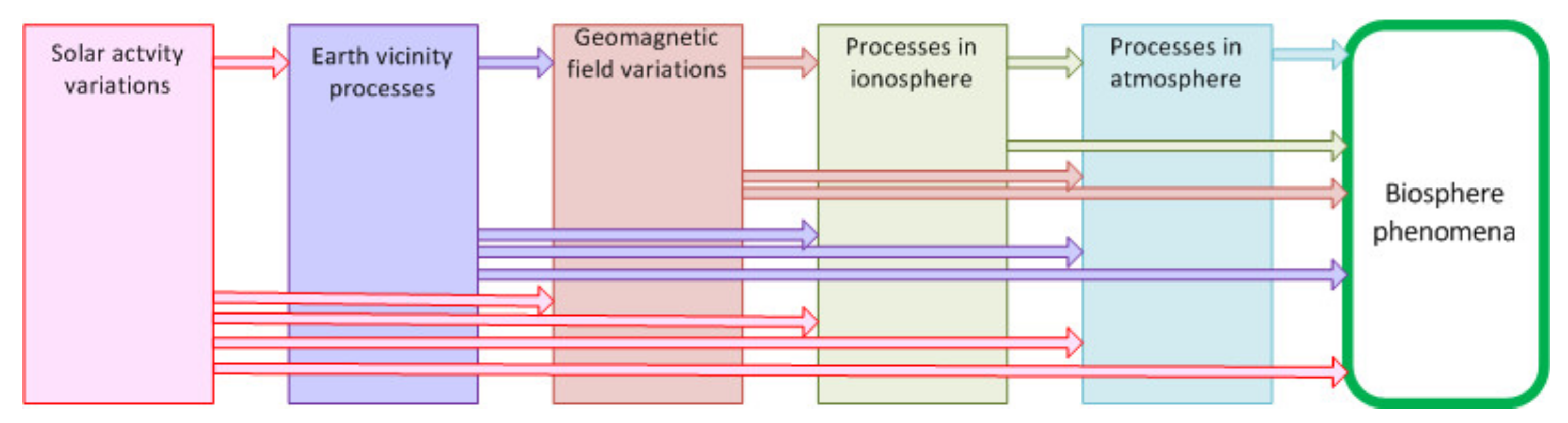
The working scheme of the representation of the natural environment (meteorological and helio-geophysical factors) is focused on the structure of the solar–terrestrial relations, which is based on the position of natural phenomena in space relative to the investigation object on the Earth’s surface—the human person:

• variations of Solar Activity SA (SA global variations and variations of SA flare components)
• variations in the characteristics of processes in the near-Earth space,
• variations in the characteristics of the geomagnetic field,
• variations in the characteristics of the ionosphere and
• variations of meteorological characteristics.

Detailed descriptions of environmental data see in Section 3.2 and in Appendix A.

Based on the proposed scheme, the structure of the studied complex of environmental factors is formed. The Weather Complex consists of two blocks—(1) Space and (2) Terrestrial Weather, divided into the listed subblocks (“Weather Complexes Blocks” in this work). The proposed scheme has the following advantages: (1) it represents an approximate outline of the natural environment (although, of course, it does not claim to be a complete representation of it), and (2) when expanding the study, it makes it easy to add new blocks of environmental characteristics.

Each of the listed blocks contains the entire set of daily statistical characteristics of each of the factors included in it. The starting hypothesis in this work is the assumption of an unknown predominant significance of any of the daily characteristics (statistics) of an environmental parameter for its role as a factor provoking a medical event (for example, the average daily value of atmosphere pressure vs. its daily variance). Each of the daily statistical characteristics of each environmental parameter is thus transformed into an independent and equal with the other studied factor.

(9)

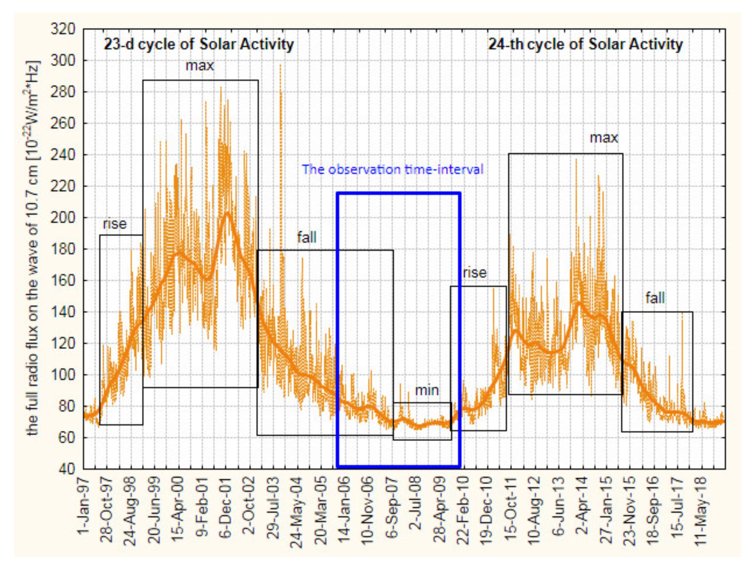
In order to avoid the errors described in paragraphs 7 and 8, we investigate the environmental variations in the interval of +/− 5 days from the date of registration of the medical event. In this work we only considered the half-interval from the (−5) day to the medical event; the investigation of it is useful for the forecast purpose. In this work, we claimed to create the scientific basis for correct environment monitoring and, thereby, for veracious special (medical) weather forecasts.

(10)

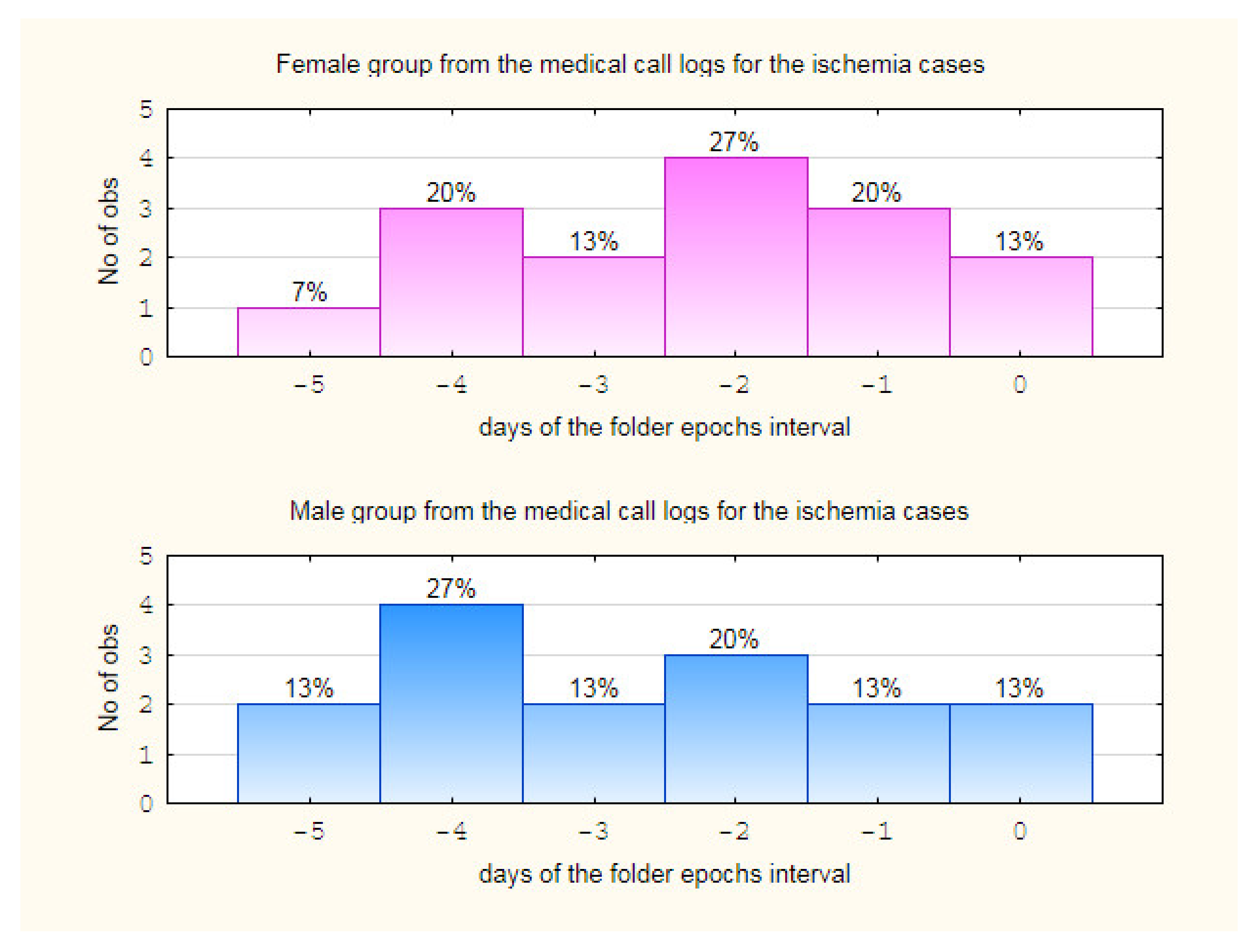
Keeping in mind the possible time discrepancies of a medical event with a moment of the distinct weather change, we are looking for the day of maximum difference of Weather Complexes (“Maximal Difference Day” in this work) in the mentioned interval.

To find the Maximal Difference Day, we use elements of the Folder Epochs Method, some elements of Cluster Analysis and the Mann-Whitney hypothesis test criterion. In detail:

• We consider the days of registration of the concrete studied categories of medical events as the key days (0 days) of the Folder Epochs Method.
• The sets of environmental parameters, which correspond to the days of registration of different categories of medical events (Middle vs. Nobody), are obviously clusters that are already formed according to a given condition: compliance with a specific medical event under study. Thus, we come to one of the tasks of Cluster Analysis: the determination of inter-cluster distances and the allocation of the maximum of them. The Euclidean inter-cluster distance we used was defined as

  $$distance\left(X,Y\right)=\sqrt{{\displaystyle \sum }_{i=1}^n{\left(x_i-y_i\right)}^2}$$

  (2)

  where $X$ and $Y$ are the studied clusters of environmental parameters sets that were registered in days of concrete different medical events, n is the number of their members and $x_i$ and $y_i$ are the values of standardized (in this paper for the seasonal median) values of environmental parameters—members of the corresponding clusters.

We propose to designate one of clusters as the “base cluster” (for example, Weather Complex, which corresponds to the “norm” of the events under study or, alternatively, to a pronounced “anomaly” under study) and determine the distance between it and the other cluster. It is also desirable to determine the level of significance of the differences in the distributions of cluster member parameters corresponding to different medical events. The nonparametric Mann–Whitney criterion is used to determine this level. The nonparametric criterion was chosen due to the discrepancy between the law of Normal Distribution and the Empirical Distribution low of a significant part of the environmental parameters included in the study (usually, the boundaries of the asymmetry coefficient: (−2,5)–(+3.15) and kurtosis coefficient: (−5,6)–(+14) in any Weather Complex that we treated). The environmental characteristics, the difference of which is unreliable by Mann–Whitney criterion, are excluded from further research. In this step, we cleared the first collection of environmental parameters from excessive amounts of them.

Each member of the Weather Complex was registered not only in one day for a specific medical event. It means that, in any concrete season, we observed some number of days with medical “norm” (Middle) and some number of days with medical “anomaly” (Nobody). The set of environmental parameters for every such day can be represented by a point (let us call it an “observation point”) in a multidimensional space which dimensions are equal to the number of these parameters. It is necessary to work with projections of these points in a straight line defining the inter-cluster distance, and then, for these projections, we have to calculate both the variance and the level of significance of similarity/difference of their distributions in relation to the Weather Complexes—Middle and Weather Complexes—Nobody. We also propose the nonparametric Mann–Whitney criterion to determine this level.

Finally, we find the day with maximal difference of the Weather Complexes sets by the maximal difference of their projection distributions in the line of the inter-cluster distance.

Thus, it is proposed to perform the following procedure:

(1)

The calculations of the distance between 2 points $\overrightarrow{X}$,$\overrightarrow{Y}$ corresponding to 2 different phenomena under study. This is the Euclidean norm of the difference between the medians (the median was calculated in the sample of days when the concrete medical event occurred) of the observed values of each environmental characteristic:

$$distance\left(X,Y\right)=\Vert X,Y\Vert =\sqrt{{{\displaystyle \sum }}_{i=1}^n{\left(x_{{0.5}_1}-y_{{0.5}_i}\right)}^2 }$$

(3)

(2)

The calculation of the guiding cosines of each difference in the medians of the observed values of each environmental characteristic:

$$\cos {\alpha }_i=\frac{x_{{0.5}_i}-y_{{0.5}_i}}{distance\left(X,Y\right)}$$

(4)

(3)

The determination of the equation of the straight line to which the distance between the points $\overrightarrow{X}$,$\overrightarrow{Y}$ belongs. The coefficients in the equation of the straight line are the calculated guide cosines.

$$\overrightarrow{t_x}=\overrightarrow{X}+\overrightarrow{\cos \alpha }\ast {\tau }_x$$

(5)

$$\overrightarrow{t_y}=\overrightarrow{Y}+\overrightarrow{\cos \alpha }\ast {\tau }_y$$

(6)

where $\overrightarrow{X}$ is the origin of coordinates set at the “base” point, τ is the position of the projection of the point of a particular observation on the straight line of the distance between the points $\overrightarrow{X}$,$\overrightarrow{Y} \mathrm{and}$ $\overrightarrow{t_x}$ is the blind variable.

(4)

The determination of the equation of the plane that is perpendicular to the described line. The coefficients in the equation of such a plane, by definition, are the coefficients of a straight line perpendicular to this plane:

$${\overrightarrow{\cos \alpha }}^T\ast \overrightarrow{t}+D=0$$

(7)

The plane contains the point of a particular observation ${\overrightarrow{X}}_{obs}$; hence:

$${\overrightarrow{\cos \alpha }}^T\ast {\overrightarrow{X}}_{obs}+D=0$$

(8)

then

$${\overrightarrow{\cos \alpha }}^T\ast {\overrightarrow{X}}_{obs}=-D$$

(9)

The equation of the plane passing through the point of a particular observation and intersecting perpendicular to the straight line of the distance between the points $\overrightarrow{X}$,$\overrightarrow{Y}$:

$${\overrightarrow{\cos \alpha }}^T\ast \left(\overrightarrow{X}+\overrightarrow{\cos \alpha }\ast \tau \right)-{\overrightarrow{\cos \alpha }}^T\ast {\overrightarrow{X}}_{obs}=0$$

(10)

The intersection of the specified plane and the straight line determines the position of the projection of the point of a particular observation in the straight line of the distance between the points $\overrightarrow{X}$,$\overrightarrow{Y}$:

$${\overrightarrow{\cos \alpha }}^T\ast \left(\left(\overrightarrow{X}+\overrightarrow{\cos \alpha }\ast \tau \right)-{\overrightarrow{X}}_{obs}\right)=0$$

(11)

$$\tau ={\overrightarrow{\cos \alpha }}^T\ast \left({\overrightarrow{X}}_{obs}-\overrightarrow{X}\right)$$

(12)

Then, the projection of the point of a particular observation in the straight line of the distance between the points $\overrightarrow{X}$,$\overrightarrow{Y}$:

$$x_{{obs}_{pr}}=\tau ={{\displaystyle \sum }}_{i=1}^{N_{Env.Param}}\cos {\alpha }_i\ast \left(x_{obs}{}_i-x_{0.5}{}_i\right)$$

(13)

We proposed to take a certain level of significance by the Mann–Whitney criterion of the null hypothesis about the similarity of the distributions of the projections of the points obtained from repeated observations of the concrete medical event on the straight line, which belongs to the distance between the points $\overrightarrow{X}$,$\overrightarrow{Y}$ as the threshold for the reliability of the difference between Weather Complexes that correspond to medical events. In this work, we use p < 0.05.

The conducted analysis allows:

• To find the day of the maximal difference of the Weather Complexes, which correspond to the different medical events.
• To find the days when such complexes did not differ (in this case, the Mann-Whitney significance level is quite high).
• To filter out the parameters whose difference is unreliable in terms of the significance of the Mann–Whitney hypothesis test criterion.
• To consider as responsible for the division of medical events into categories only those environmental parameters that would differ by Mann–Whitney criterion when they correspond to the different categories of the medical events.

(11)

We investigate—within the interval of the folder epochs—the behavior of some parameters that are different when they correspond to different medical events.

The scheme of the method is illustrated in Figure 2.

The algorithm for the implementation of the above-described method we developed specially for this work and applied it by VBA STATISTICA.

The investigation points in the presented work are:

• The day of the Weather Complexes maximal difference when they corresponded to the different medical events: Nobody and Middle—Maximal Difference Day in this work. We have investigated the first part of the folder epochs interval—from the (–5) day to the key day—for the scope of the investigation of forecast perspectives.
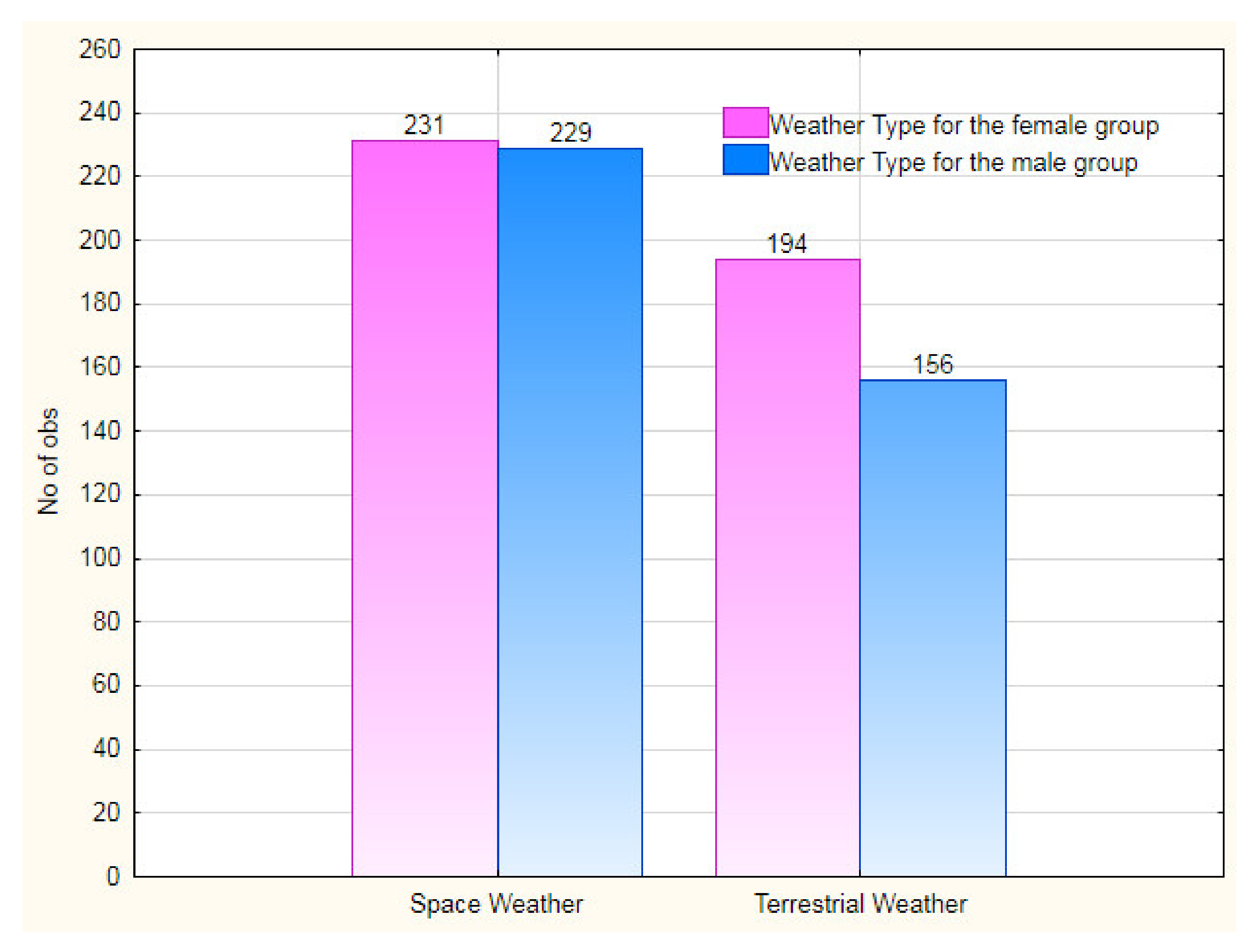
• The ratio of Space Weather characteristics to Terrestrial Weather characteristics, which differed when corresponding to the different medical events in the Maximal Difference Days.
• The distribution of the above-mentioned characteristics by Weather Complex blocks. These blocks relate to the different environmental fields.
• The lists of the concrete environmental characteristics that were different when they were registered in the days of the different medical events.
• The plot of the timeline—behaviors of some selected environmental characteristics as an example of such behavior features.

2.2. Materials

2.2.1. Medical Data

The medical material is the daily number of ischemia cases in the one of Saint Petersburg districts (from the call logs of medical officials). We analyzed the environmental circumstance of the two alternative events: the days with ischemia case normal numbers (“Middle” in this work) vs. the days of such case absences (“Nobody” in this work). “Middle” we calculated separately for ischemia cases in different gender and age groups, and it means the number of call for ischemia cases in the frame of the seasonal median deviation for these groups. Only those days when “Middle” coincides for different ages within the gender group were selected for the study. However, “Nobody” means the empty days for these events at all—nobody in the men group and the same in the women group.

The observed time interval: 19.12.2005–31.12.2009. The whole number of ischemia cases—15,122. The samples of investigated days of different medical events in different calendar seasons have commensurate sizes (

Table 1. The number of the medical events under study in the different seasons in the observing time interval.

Calendar Season	Nobody	Male Group Middle	Female Group Middle
winter 2005–2006	11	20	23
spring 2006	21	19	32
summer 2006	22	17	23
autumn 2006	20	28	28
winter 2006–2007	19	26	33
spring 2007	15	15	35
summer 2007	23	26	31
autumn 2007	18	8	29
winter 2007–2008	13	25	36
spring 2008	20	31	31
summer 2008	20	20	23
autumn 2008	17	14	34
winter 2008–2009	16	28	33
spring 2009	23	26	29
summer 2009	7	12	22
autumn 2009		14	21
winter 2009–2010		7	7

). We have to note the absence of “Nobody” events in autumn 2009 and winter 2009–2010.

2.2.2. Environmental Data

(1)

Daily indices of Solar Activity (SA) global variations (the full radio flux on λ = 10.7 cm, Wolf-number, the daily sum of the area of all observed sunspots and the number of the new Active Regions per day) [47]—GlobalSun conditional block in this work.

(2)

Daily characteristics of the SA flare-component in various bands of the electromagnetic spectrum (optical-, radio- and X-ray-band) [47]—SolarFlare conditional block in this work.

(3)

Daily variations of Interplanetary Space characteristics in the near-Earth space (e^–, p⁺ and α-particle fluxes) [48]—EarthVicinity conditional block in this work.

(4)

Daily Geomagnetic Field (GF) variations (the total GF vector in the near-Earth space (GOES orbit), the component of GF that is perpendicular to the Earth’s orbit plane in the near-Earth space (GOES orbit); K–indices on high terrestrial latitudes; K–indices on middle terrestrial latitudes and GF x-,y- and z-components on the latitude of Saint Petersburg) [48,49]—GeoMag conditional block in this work.

(5)

Ionosphere phenomena (sudden ionosphere disturbances) [50]—ion conditional block in this work.

(6)

Atmosphere parameters (the atmosphere pressure, the low nebulosity, the wind speed, the humidity, the air temperature, the dew point temperature and weight oxygen content in the air) (Saint Petersburg meteorology station, #26063 (59°58′ N 30°18′ E))—respectively, Baric, Humidity, Temperature and Oxy conditional blocks in this work.

These environmental characteristics for days of ischemia cases were investigated in frames of exact terrestrial calendar seasons close to the SA minimum between the 23rd and 24th cycles (Figure 3).

The detailed list of the environmental parameters included in this work were put in Appendix A.

3. Results

Our investigation—in the frame of the observing time interval—discovered some gender features of human relations to the environmental variations. These features are partly common for people from the different gender groups and partly quite various. We have highlighted—at the concrete investigation points—these similarities and conformities below under the investigation points those were described in Section 2.1.

3.1. The Day of the Weather Complexes Maximal Difference When They Corresponded to the Different Medical Events Nobody and Middle in the First Part of the Folder Epochs Interval—From the (−5) Day to the Key Day

We discovered the little dominance of the (−4) day and (−2) day as the Maximal Difference Days in the days line of the half-interval of folder epochs. The dominance is small in the frame of 15 calendar seasons—the Maximal Difference Days were revealed in each season—but give some hint for the careful investigation of these days for the forecast purpose (Figure 4). Additionally, one can note the small tendency of the days’ distribution center to the key day (0-day) in the female group.

The Maximal Difference Days varied from season to season in alternative gender groups, but in 40% of seasons these days, they were the same in the male and female groups (

Table 2. The list of Weather Maximal Difference Days in concrete seasons and concrete solar activity phases.

General Season	Concrete Season	Solar Phase	Maximal Weather Difference Day (Female Group)	Maximal Weather Difference Day (Male Group)
winter	winter 2005–2006	SolarFall	−4	−2
winter	winter 2006–2007	SolarFall	−2	−2
winter	winter 2007–2008	SolarFall	−2	−2
spring	spring 2006	SolarFall	−1	−1
spring	spring 2007	SolarFall	0	0
summer	summer 2006	SolarFall	−3	−4
summer	summer 2007	SolarFall	−5	−1
autumn	autumn 2006	SolarFall	−2	−3
autumn	autumn 2007	SolarFall	−1	−4
spring	spring 2008	CloseToMin	−1	−4
spring	spring 2009	CloseToMin	0	0
summer	summer 2008	CloseToMin	−4	−5
summer	summer 2009	CloseToMin	−2	−4
autumn	autumn 2008	CloseToMin	−4	−5
winter	winter 2008–2009	SolarMin	−3	−3

Solar phases were the fall branch (SolarFall) of solar activity 23rd cycle, the solar minimum (SolarMin) between the 23rd and 24th cycles and the vicinity of the solar minimum (CloseToMin) from the both side of this minimum.

).

The mentioned above coincidences of Maximal Difference Days went through the whole 2006 year (the phase of the solar activity fall (Figure 3) and then matched twice—in spring 2009 and winter 2008–2009. The reason of such coincidence indicates the careful investigation of it but is outside the frame of the presented work. Additionally, one can note that in those seasons when Maximal Difference Days differed between gender groups the mentioned days were closer to the day of the medical event (key day) in the female group. This fact appeared in 47% of cases in various phases of the solar activity cycle: spring 2007, from autumn 2007 to spring 2008 and from autumn 2008 to spring 2009. When called to mind the mentioned above tendency of these days’ distribution center to the key day in the female group, we may suppose the nearness of the medical event to the day of maximal weather variation in the female group. Therefore, we may assume the more sharp reaction of a female organism to the weather conditions change.

3.2. The Ratio of Space Weather Characteristics to Terrestrial Weather Characteristics Which Differed When Corresponded to the Different Medical Events in the Maximal Difference Days

We investigated the environmental characteristics—these parameters have different values that corresponded to the different medical events; those were observed in the Maximal Difference Days, which were revealed in each season. Therefore, we could detect the overweight of the Space Weather parameters part over the Terrestrial Weather part in those days (Figure 5).

The ratio between the Weather Types in the Maximal Difference Days shows the dependence from the solar phases and seasons and differs between investigated gender groups (Figure 6 and Figure 7).

Figure 6 shows the significant overweight of SW parameters over TW parameters, which were different at different medical events in the Female group on the 23rd solar activity cycle fall phase. In the Male group, medical events were mostly under SW parameter variations in any calendar season and any solar phase, except only summer seasons in the solar fall phase—those are summer 2006 and summer 2007 (Figure 7). Additionally, the summer seasons are interesting because of another reason—the ratios between SW and TW parameters are alternative in the alternative gender groups. This difference is marked by the red contours in Figure 6 and Figure 7. The reason of this fact is outside the frame of this work but is exactly a good base for the careful investigation of the gender features in a human relation to the environmental variations of different conditions—different solar phases at the same calendar seasons. Exact alternative were Weather Complexes structures when they corresponded to different medical events in the alternative gender groups in the solar minimum phase. The difference is marked by green circles in Figure 6 and Figure 7. One can see the absolute absence of SW parameters in the Female group and such an absence of TW parameters in the Male group.

Of course, we tried to find out the environmental characteristics that were significant different at the different medical events and were common for the both gender groups. The ratio between the SW and TW parameters of such characteristics is more balanced than the ratio mentioned above (Figure 8).

The distribution of these environmental characteristics by the calendar seasons and solar activity phases is shown in Figure 9.

Figure 9 shows the overweight of common TW parameters over common SW parameters in the steady seasons—summers and winters in the solar activity fall branch, as well as in the summertime of the solar activity phase close to the solar minimum. The fact of the summer’s similarity in this field shows the way for the investigation of the above-mentioned phenomenon—the alternative ratios between SW and TW parameters in the alternative gender groups that were shown in Figure 6 and Figure 7. The reason for this phenomenon is that we should search in the particularity of SW parameters in the different phases of the solar activity.

3.3. The Distribution of the Mentioned above Characteristics by Weather Complexes Blocks. These Blocks Relate to the Different Environmental Fields

The detailed investigation of Weather Complexes structure in Maximal Difference Days shows the bimodal distribution of the mentioned above SW and TW parameters—the geomagnetic block in the Space Weather complex and the humidity block in the Terrestrial Weather complex are leading among all revealed parameters, summarized parameters for the both gender groups (Figure 10), as well as among parameters that are common for the different gender groups (Figure 11).

3.4. The Lists of the Concrete Environmental Characteristics That Are Different When They Were Registered in the Days of Different Medical Events

Here, we should show only those environmental parameters that were revealed in more than two calendar seasons or more than in two solar activity cycle phases.

For the parameters common for both gender groups, there was not found out such frequent appearances of the concrete parameters. Only the daily range and the daily standard deviation of the total magnetic field in the near-Earth space (satellite GOES orbit) were repeated twice in autumns of the solar activity fall phase. Of course, we must note that, in the frame of our investigation, we had only these two autumns (see Table 2) in this solar phase. Therefore, this fact gives us the next hint for the careful investigations of autumns in solar fall phase. Other environmental parameters differed by their value when corresponding to different medical events, mostly one time for each parameter per calendar season of the concrete year. Such diversity of Weather Complex factors that may be responsible for the circumstance of medical events in different conditions—the matching of calendar season features (Terrestrial Weather) with solar activity phase features (Space Weather)—may lead us to the hypothesis of the equality and interchangeability of environmental parameters that can impact human organism. One can call to mind the repeating of Maximal Difference Days for Weather Complexes (Figure 4 and Table 2) and note its structure difference from season to season for assuming this hypothesis.

Between the parameters those were specific for the concrete gender group, we found few repeated appearances of some of them in quite different calendar seasons but in the same solar activity phases (

Table 3. The list of the revealed parameters that were different at the moments (the days) of the different medical events, Nobody and Middle, and were specific for each of different gender group.

Gender Group	Solar Activity Phase	Calendar Season	Environmental Parameter	Weather Type
Female	SolarFall	2 Winters, Spring	proton flux E = (4–9 MeV)—daily maximum	Space Weather
		Spring, Summer Autumn	total magnetic field in the Earth Vicinity—daily maximum	Space Weather
		Summer, Winter, Spring, Autumn	3-hourly K indices high-latitude station monitoring Earth’s magnetic field—daily maximum	Space Weather
		Summer, Winter, Autumn	3-hourly K indices from high–latitude station monitoring Earth’s magnetic field—daily median	Space Weather
		2 Autumns, Winter	3-hourly K indices from the middle—latitude station monitoring Earth’s magnetic field—daily median	Space Weather
		Winter, Spring, Summer	Temperature of Dew Point—standard deviation, coefficient of oscillation	Terrestrial Weather
Male	SolarFall	Winter, Spring, Summer	Geomagnetic Field Magnitude y-component, (Saint Petersburg latitude)—daily median	Space Weather
		2 Summers, Winter	Geomagnetic Field Magnitude z-component, (Saint Petersburg latitude)—daily median	Space Weather
		2 Winters, Autumn	Relative Humidity—daily median	Terrestrial Weather
		2 Winters, Autumn	Relative Humidity—daily min	Terrestrial Weather
	CloseToMin	Spring, Winter, Summer	3-hourly K indices from the middle-latitude station monitoring Earth’s magnetic field—daily coefficient of oscillation	Space Weather
		2 Springs, Summer	Temperature of Dew Point—daily minimum	Terrestrial Weather

).

Table 3 shows the overweight of large-scale space parameters (geomagnetic, high- and middle-geo-latitudes), which were different at the different medical events in the Female group vs. local-scale parameters (geomagnetic on the latitude of Saint Petersburg) in the Male group in the solar activity fall phase.

3.5. The Plot of the Time–Behaviour of Some Selected Environmental Characteristics as the Example of Such Behaviour Features

The time–behavior of the revealed environmental parameters is always significant differs when these parameters were registered near the day of the concrete different medical events. In Figure 12, we show an example of such behavior for the parameter that is common for the both gender groups—the daily standard deviation of the total magnetic field in the near-Earth space (GOES orbit). One can see the dramatic difference of the timelines of this Space Weather characteristic when it was recorded near the days of the “normal” number of calls for ischemia (Middle—season norm) in both gender groups vs. the days of absolute absence of such calls (Nobody). Additionally, these lines show slight difference between gender groups events. All declinations from the seasonal norm (0: line on the plot of the standardized value) are small—within the frames of the seasonal standard deviation, but the behavior lines are obviously specific. The discussion of the geomagnetic field behavior specialty is outside frame of the presented work, but we have to note that, in our previous works [28,29], we have seen the rise of the geomagnetic field daily spread that corresponded to the good cardio-situation in our city.

4. Discussion

The results of our work have shown the multiparametric feature of the environmental impact on the human organism status. Often researchers investigate only one environmental factor that can impact the human or any other living organism [6,17,19,21,22,25]. Some researchers take a few environmental parameters for the investigation [14,20,23,26], but these environmental parameters usually are predefined as obvious factors that can affect the human organism. Frequently, this ensemble of factors consists of the air temperature, air pressure plus in different works one of space weather parameters is added [20,24,26]—usually, the geomagnetic disturbances are added to the investigation [26]. These works are very informative, especially those of them in which not popular environmental parameters were combined for the study [23]. Our approach to this issue—the consideration of the most holistic collection of the environmental characteristics that includes, together, space and terrestrial weather in various manifestations without any predefined selection—permit discovering, firstly, a complex environmental characteristics sample that could jointly impact people with ischemia and, secondly, permit discovering some unexpected environmental parameters that are significance for people with ischemia. Some unpredictability was in the predomination of the humidity characteristics in the terrestrial part of factors those affect ischemic people. We have to pay special attention to the temperature of the dew point. This parameter is complex; it describes the combination of the relative humidity and the air temperature, so, by the mentioned parameter, we can again note the complexity of environmental impact on the human health.

Our decision to investigate the days those were previous to the medical events permits us to discover the day when Weather Complexes were maximally different in their relation to the normal number of the ischemia cases vs. the absence of them. This discovering gives us a way to forecast ischemia cases by careful study of such days. It is important that the study of the closeness of such days of medical events discovers a dependence on the gender groups of ischemic people under investigation. Usually, the researchers investigate the exact day of the medical event [8,9,10,11,12,17,20,21,22,23,24,25,26] so they cannot offer a scheme for the forecast of the environmental variations that can cause the medical events.

Our approach to the study that permit us to consider not only daily averages—that is common [19,20,21,22,24]—but to study all daily statistics shows the common for people’s—any gender group—reactions to the standard deviation of the total magnetic field vector value, which was measured in the near-Earth space (GOES orbit).

Our decision to investigate the probable influence of the geomagnetic variations on the different gender groups when these variations were measured in the different geomagnetic points—so they can describe the geomagnetic situation as the global factor (near-Earth space, high and middle latitudes) or as the local factor (exact Saint Petersburg latitude)—permit us to discover the gender differences in the sensitivity to these variations. It is a fact that females reacted to large-scale geomagnetic variations, and males reacted to the local-scale geomagnetic variations. Often [6,8,9,10,11,12,26], the geomagnetic characteristics are investigated only in a local geo-point of study or investigated only on planetary-scale geomagnetic indexes [14].

Our approach to the study with the consideration of the different components of the geomagnetic field at the local point (x-, y- and z-components at the Saint Petersburg latitude) helped us to discover the reaction of the male group to the daily median value of the y- and z-components and not the x-component, which variations usually detect geomagnetic storms [6].

We discovered the significance of the quite different parameters for ischemic people depends on the matching of the calendar season with the phase of the solar activity. We offer the hypothesis of the equality and interchangeability of environmental parameters that can impact the human organism—the same human reaction on different kinds of the environmental impacts, as we have mentioned in the Materials and Methods section (Section 2.1, error #4 in the list of probable study’s errors). This hypothesis we have assumed when saw the changing of environmental factors collection content from season to season of the concrete years. We never meet such a hypothesis in the works of other researchers.

Our results show the way to the detailed study of the geomagnetic spread-out characteristics in autumns of solar fall phases. The repeating of the spread statistics of the total magnetic field in the Earth vicinity as the factor that is common for both gender groups in similar seasons and in the same solar phase leads us to such study. We never meet such results in the works of other researchers.

We found out the rising of the daily spreading of the total magnetic field vector value in the near-Earth space (GOES orbit) before the 2 days of absolute absence of the ischemia cases in any gender group vs. the falling of this environmental parameter before 1 day to the normal number of mentioned cases. We never meet such results in the works of other researchers, but we found such an unexpected effect in our previous works [28,29].

We are glad that our investigation with the unprejudiced selection of the environmental parameters shows the significance of the geomagnetic field variations of ischemic people. This fact proves the correctness of other research works [6,7,8,9,10,11,12,13,14,15] and adds new features to the investigation of the geomagnetic effects on human life.

The above results were obtained in the relatively short time interval that was close to the solar activity minimum between the 23rd and 24th cycles. The length of this interval is not enough for ultimately confident conclusions about the human organism in relation to environmental variations on a large scale. However, we must note that our time interval of observation (4 years) was not so much shorter than some mentioned in the introduction to this article authors have: 1 year in Reference [6], 2 years and 3 months in Reference [21], 4 months in Reference [24], 1 month in Reference [12] and 2 months in Reference [11]. There are longer time intervals under investigation, [14,25] but these researchers did not take into account the calendar seasons and solar activity phase relations of their studies.

Additionally, the number of the investigated ischemia cases—15,122—allowed us be confident in these results to highlight the direction of careful future studies for some concrete points.

These points are:

• The sharp reaction of a female organism to weather conditions changes. This conclusion we assumed from the closeness of Weather Complexes Maximal Different Days to the medical events in the Female group (Figure 4 and Table 2).
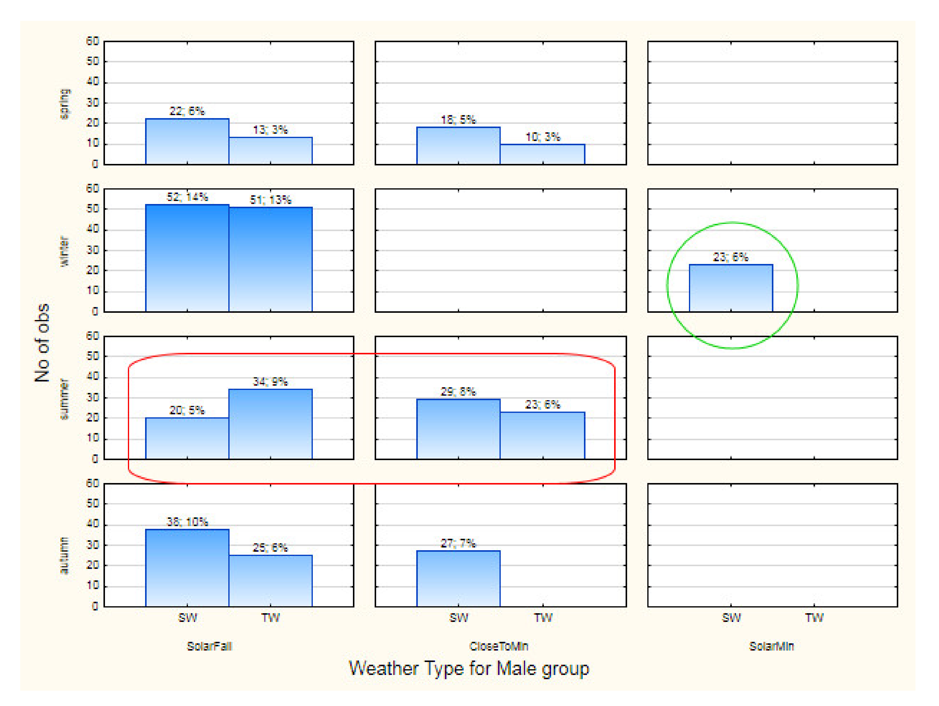
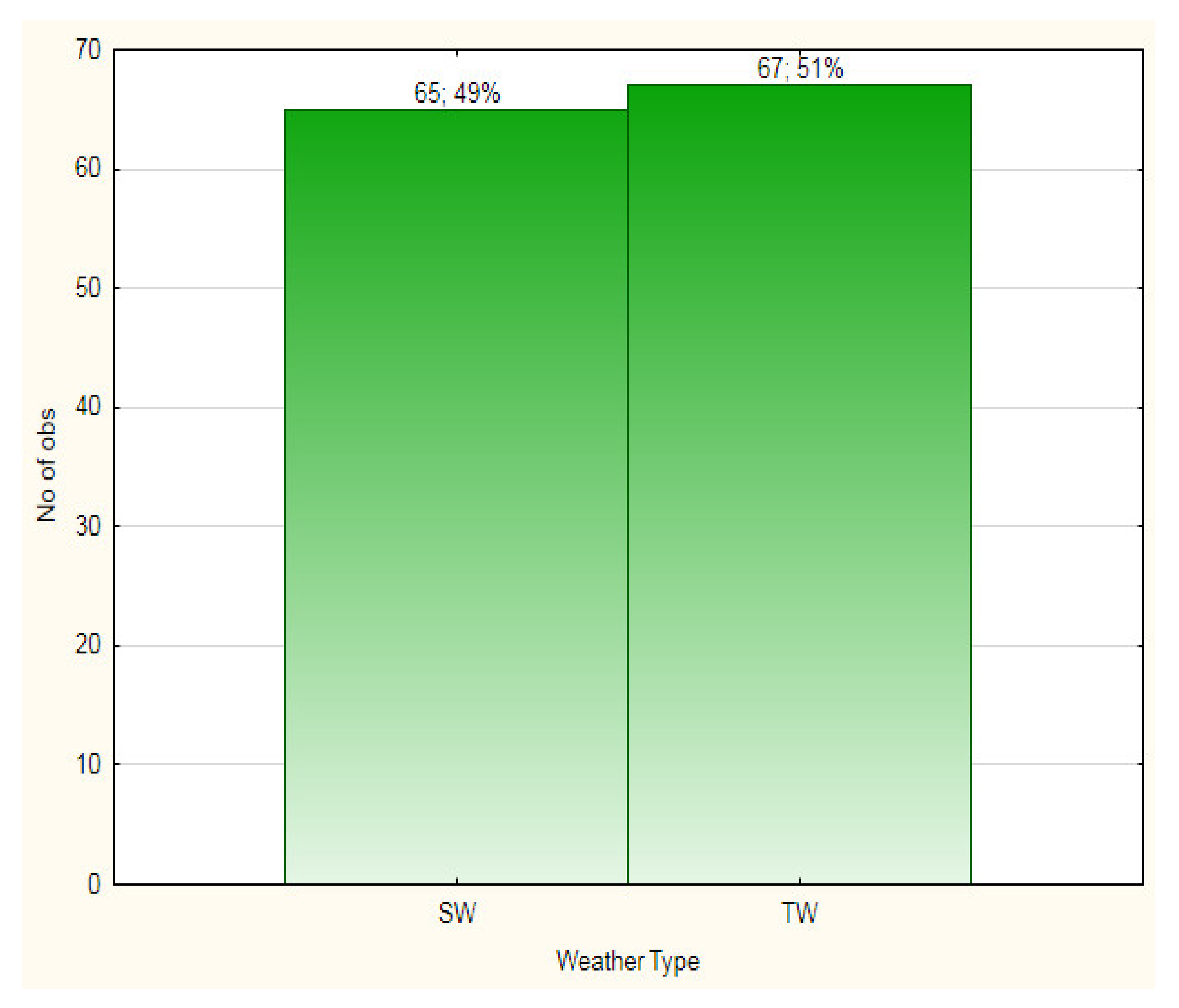
• The classification of the combinations of calendar seasons with solar activity phases cause different weights of Space and Terrestrial types of weather in Weather Complexes of environmental factors, which can impact the human organism. We can see this unbalance from distributions of the weather types by calendar seasons and solar activity phases (Figure 6 and Figure 7).
• The careful study of geomagnetic factors of Space Weather and humidity factors of Terrestrial Weather. These parameters were highlighted from the distributions of factors by environmental blocks (Figure 10 and Figure 11).
• The detailed study of the geomagnetic spread characteristics in the autumns of the solar fall phases. The repeating of the spread statistics of the total magnetic field in the Earth vicinity as the factor that is common for both gender groups in the similar seasons and in the same solar phase leads us to such study (Section 3.3 and Section 3.4 in the Results).
• The verification of hypothesis of the equality and interchangeability of environmental parameters that can impact human organism. This hypothesis we assumed when we saw the changing of environmental factors collection from season to season of the concrete years (Section 3.3 in the Results).
• The clarification of the fact of female reaction to large-scale geomagnetic variations when the male reaction was registered on the local-scale geomagnetic variations. This fact was evident as the result of study of the environmental factors specific for each gender group separately (Table 3).
• The verification of the good influence of small geomagnetic field variations to human health (Figure 12). This result is unexpected but appears not only in our work [28,29].

5. Conclusions

• The presented work shows the results of the complex study of the holistic environmental impact (Weather Complex impact) on the human organism.
• The comparing of the Weather Complexes in their relation to the days with different numbers of the ischemia cases in the frames of the study discovered the days of the maximal difference of these complexes (Maximal Difference Days) before the exact days of the registration of the concrete numbers of the ischemia cases. This fact is useful for the forecast purposes.
• The dissimilarity of the Maximal Difference Days for the different ischemic people gender groups led to the necessity of gender-targeted forecasts of the environmental status for the different medical events of the ischemia cases.
• The unprejudiced selection of the environmental parameters for the study shows the primary importance of the geomagnetic parameters as the Space Weather factors and the humidity parameters as the Terrestrial factors for the ischemia outcomes.
• The including of the environmental parameters daily statistics to the study shows the importance of point statistics and spread statistics in different circumstances.
• The investigation of different circumstance that is described by the different combinations of the calendar seasons with the phases of the solar activity cycle leads to the hypothesis of the equality and interchangeability of environmental parameters which can impact the human organism.
• The investigation of different circumstance that is described by the different combinations of the calendar seasons with the phases of the solar activity cycle discovers—in the frames of our work—the different weights of Space and Terrestrial types of weather in Weather Complexes in such combinations.
• The daily spread of the geomagnetic total vector value in near-Earth space turned out—in the frames of our study—to be important for the both ischemia-people gender-groups in the autumns of solar activity cycle falling phase.
• The investigation of the behavior of the daily spread of the total vector value in near-Earth space before the days of different numbers of the ischemia cases discovers—in the frames of our work—the rising of this spread before two days to the absence of the ischemia cases contra falling of it before one day to the normal value of these cases. That fact was noted for the both ischemia-people gender-groups in the autumns of solar activity cycle falling phase.
• The including of the different geomagnetic points to the study discovers—in the frames of our work—the importance of the local geomagnetic daily median for the ischemia-people male group contra the large-scale geomagnetic daily point-statistics (maximum and median) for the female group.
• The including of three geomagnetic field components in the local terrestrial point (Saint Petersburg latitude) to the study discovers—in the frames of our investigation—the importance of y- and z-components for the ischemia-people male group.
• The results of the presented study mostly show the perspective for the expanded investigation. However, the representativity of ischemia cases sample allows us to confide in accuracy of the planned study directions.

References

- Tchijevsky, A.L. Ueber die Wechselbeziehungen zwischen der periodischen Tatigkeit der Sonne und den Cholera und Grippe Epidemien. Dtsch.–Russ. Med. Z. 1927, 3, 511–539. [Google Scholar]
- Tchijevsky, A.L. Kosmische Einfluesse, die Entstehung und Verbreitung von Massepsyshoseh beguenstigen. Dtsch.–Russ. Med. Z. 1928, 17, 1–89. [Google Scholar]
- Tchijevsky, A.L. La radiation cosigue comme facteur biologique. Resultats des recherches experimentales de l’influence de la radiation cosmique, solaire et astrale sur les cellules et les tissus. Bull. L’Association Int. Biocomigue Toulon 1929, 13, 245–250. [Google Scholar]
- Tchijevsky, A.L. A propos de I’influence de l’active solar periodique sur le movement des masses humaines11, 57–62. La Cote d’Azur Med. Toulon 1929, 11, 57–62. [Google Scholar]
- Vladimirski, B.M.; Temurjantz, N.A. The Influense of Solar Activity on the Biosphere–Noosphere; IIEPU: Moskow, Russia, 2000; p. 374. [Google Scholar]
- Chernouss, S.; Vinogradov, A.; Vlassova, E. Geophysical Hazard for Human Health in the Circumpolar Auroral Belt: Evidence of a Relationship between Heart Rate Variation and Electromagnetic Disturbances. Nat. Hazards 2001, 23, 121–135. [Google Scholar] [CrossRef]
- Unger, S. The Impact of Space Weather on Human Health. Biomed. J. Sci. Tech. Res. 2019, 22, 16442–16443. [Google Scholar] [CrossRef]
- Belisheva, N. The Effect of Space Weather on Human Body at the Spitsbergen Archipelago; IntechOpen: London, UK, 2019. [Google Scholar] [CrossRef] [Green Version]
- Belisheva, N.K.; Vinogradov, A.N.; Vashenyuk, E.V.; Tsymbalyuk, N.I.; Chernous, S.A. Biomedical research on Svalbard as an effective approach to studying the bioefficiency of space weather. Herald KSC RAS 2010, 1, 26–33. [Google Scholar]
- Belisheva, N.K.; Martynova, A.A.; Pryanichnikov, S.V.; Solov’evskaya, N.L.; Zavadskaya, T.S.; Megorsky, V.V. Connection of the Parameters of the Interplanetary Magnetic Field and the Solar Wind in the Polar Cusp Region with the Psychophysiological State of the Inhabitants of Arch. Spitsbergen. Herald KSC RAS 2018, 4, 5–24. [Google Scholar] [CrossRef]
- Samsonov, S.; Parshina, S. Space weather in the 11-year solar cycle and cardio-sensitivity of volunteers in the middle latitudes. IOP Conf. Ser. Earth Environ. Sci. 2021, 853, 012028. [Google Scholar] [CrossRef]
- Kodochigova, A.I.; Samsonov, S.N.; Polidanov, M.A. Psychological characteristics of the Heliomed 2 project volunteers and geomagnetic disturbance at high latitudes. IOP Conf. Ser. Earth Environ. Sci. 2021, 853, 012027. [Google Scholar] [CrossRef]
- Stoupel, E. Considering space weather forces interaction on human health: The equilibrium paradigm in clinical cosmobiology is it equal? J. Basic Clin. Physiol. Pharmacol. 2015, 26, 147–151. [Google Scholar] [CrossRef] [PubMed]
- Stoupel, E.; Radishauskas, R.; Bernotiene, G.; Tamoshiunas, A.; Virvichiute, D. Blood troponin levels in acute cardiac events depends on space weather activity components (a correlative study). J. Basic Clin. Physiol. Pharmacol. 2018, 29, 257–263. [Google Scholar] [CrossRef] [PubMed]
- Stoupel, E.G.; Petrauskiene, J.; Kalediene, R.; Sauliune, S.; Abramson, E.; Shochat, T. Space weather and human deaths distribution: 25 years’ observation (Lithuania, 1989–2013). J. Basic Clin. Physiol. Pharmacol. 2015, 26, 433–441. [Google Scholar] [CrossRef] [PubMed]
- Ferrari, F.; Szuszkiewicz, E. Cosmic rays: A review for astrobiologists. Astrobiology 2009, 9, 413–436. [Google Scholar] [CrossRef] [PubMed]
- Abalyaev, A.Y.; Grunskaya, L.V.; Leshchev, I.A. Research and forecasting of the influence of the Earth’s electromagnetic field on the accident rate on public roads. IOP Conf. Ser. Earth Environ. Sci. 2021, 853, 012033. [Google Scholar] [CrossRef]
- Minina, E.N.; Bobrik, Y.V.; Ponomarev, V.A. The change of the skin electroconductivity and cardiointervalography inidicators under the influence of different physical factors. IOP Conf. Ser. Earth Environ. Sci. 2021, 853, 012031. [Google Scholar] [CrossRef]
- Cifra, M.; Apollonio, F.; Liberti, M.; Mir, L.M. Possible molecular and cellular mechanisms at the basis of atmospheric electromagnetic field bioeffects. Int. J. Biometeorol. 2021, 65, 59–67. [Google Scholar] [CrossRef] [Green Version]
- Ochiai, A.M.; Gonçalves, F.L.T.; Ambrizzi, T.; Florentino, L.C.; Wei, C.Y.; Soares, A.V.N.; De Araujo, N.M.; Gualda, D.M.R. Atmospheric conditions, lunar phases, and childbirth: A multivariate analysis. Int. J. Biometeorol. 2012, 56, 661–667. [Google Scholar] [CrossRef]
- Cui, L.; Geng, X.; Ding, T.; Tang, J.; Xu, J.; Zhai, J. Impact of ambient temperature on hospital admissions for cardiovascular disease in Hefei City, China. Int. J. Biometeorol. 2019, 63, 723–734. [Google Scholar] [CrossRef]
- Dohmen, L.M.E.; Spigt, M.; Melbye, H. The effect of atmospheric pressure on oxygen saturation and dyspnea: The Tromsø study. Int. J. Biometeorol. 2020, 64, 1103–1110. [Google Scholar] [CrossRef] [PubMed] [Green Version]
- Kourtidis, K.; André, K.S.; Karagioras, A.; Nita, I.-A.; Sátori, G.; Bór, J.; Kastelis, N. The influence of circulation weather types on the exposure of the biosphere to atmospheric electric fields. Int. J. Biometeorol. 2021, 65, 93–105. [Google Scholar] [CrossRef] [PubMed]
- Makowiec-Dąbrowska, T.; Gadzicka, E.; Siedlecka, J.; Szyjkowska, A.; Viebig, P.; Kozak, P.; Bortkiewicz, A. Climate conditions and work-related fatigue among professional drivers. Int. J. Biometeorol. 2019, 63, 121–128. [Google Scholar] [CrossRef] [Green Version]
- Yang, Z.; Wang, Q.; Liu, P. Extreme temperature and mortality: Evidence from China. Int. J. Biometeorol. 2019, 63, 29–50. [Google Scholar] [CrossRef] [PubMed]
- Sasonko, M.L.; Ozheredov, V.A.; Breus, T.K.; Ishkov, V.N.; Klochikhina, O.A.; Gurfinkel, Y.I. Combined influence of the local atmosphere conditions and space weather on three parameters of 24-h electrocardiogram monitoring. Int. J. Biometeorol. 2018, 63, 93–105. [Google Scholar] [CrossRef]
- Golovina, E.; Trubina, M.; Stupishina, O.; Misyura, O. Influence of the urban atmosphere on human health. In Proceedings of the 15th International Congress of Biometeorology & International Conference on Urban Climatology, Sydney, Australia, 8–12 November 1999. [Google Scholar]
- Stupishina, O.M.; Golovina, E.G. Investigation of Correspondence Between Environmental Parameter Complex and Human Body Status. In Proceedings of the V International Conference Atmosphere, Ionosphere, Safety, Kaliningrad, Russia, 19–25 June 2016; Karpov, I.V., Borchevkina, O.P., Eds.; Immanuil Kant Baltic Federal University Press: Kaliningrad, Russia, 2016; pp. 263–268. [Google Scholar]
- Stupishina, O.M.; Golovina, E.G. Detection and Monitoring of Environmental Factors those can be Responsible for the Cardio-Catastrophs. In Proceedings of the VI International Conference Atmosphere, Ionosphere, Safety, Kaliningrad, Russia, 3–9 June 2018; Karpov, I.V., Borchevkina, O.P., Eds.; Immanuil Kant Baltic Federal University Press: Kaliningrad, Russia, 2018; pp. 218–235. [Google Scholar]
- Stupishina, O.M.; Golovina, E.G.; Noskov, S.N. The relation of the human cardiac-events to the environmental complex variations. IOP Conf. Ser. Earth Environ. Sci. 2021, 853, 012029. [Google Scholar] [CrossRef]
- Plyaskin, V. Simulation of Particle Fluxed in the Earth’s vicinity. Int. J. Mod. Phys. A 2002, 17, 1733–1741. [Google Scholar] [CrossRef]
- Iron Is Everywhere in Earth’s Vicinity, Suggest Two Decades of Cluster Data. Available online: https://sci.esa.int/web/cluster/-/iron-is-everywhere-in-earth-s-vicinity-suggest-two-decades-of-cluster-data (accessed on 16 December 2021).
- Nitta, N.V.; Mulligan, T.; Kilpua, E.K.J.; Lynch, B.J.; Mierla, M.; O’Kane, J.; Pagano, P.; Palmerio, E.; Pomoell, J.; Richardson, I.G.; et al. Understanding the Origins of Problem Geomagnetic Storms Associated with “Stealth” Coronal Mass Ejections. Space Sci. Rev. 2021, 217, 82. [Google Scholar] [CrossRef] [PubMed]
- Cowley, S.W.H. Magnetosphere-ionosphere interactions’: A tutorial review. In Magnetospheric Current Systems; Geophysical Monograph Series; Ohtani, S.-I., Fujii, R., Hesse, M., Lysak, R.L., Eds.; American Geophysical Union: Washington, DC, USA, 2000; Volume 118, pp. 91–108. [Google Scholar] [CrossRef] [Green Version]
- Kunduri, B.S.R.; Baker, J.B.H.; Ruohoniemi, J.M.; Coster, A.J.; Vines, S.K.; Anderson, B.J.; Shepherd, S.G.; Chartier, A.T. An Examination of Magnetosphere-Ionosphere Influences during a SAPS Event. Geophys. Res. Lett. 2021, 48, e95751. [Google Scholar] [CrossRef]
- Khazanov, G.V. Why Atmospheric Backscatter Is Important in the Formation of Electron Precipitation in the Diffuse Aurora. J. Geophys. Res. Space Phys. 2021, 126, e29211. [Google Scholar] [CrossRef]
- Haigh, J.D. The impact of solar variability on climate. Science 1996, 272, 981–984. [Google Scholar] [CrossRef] [PubMed]
- Haigh, J. Solar variability and climate. In Space Weather: Research towards Applications in Europe; Lilensten, J., Ed.; Springer: Dordrecht, The Netherlands, 2007; pp. 65–81. [Google Scholar]
- Werner, K. Schmutz Changes in the Total Solar Irradiance and climatic effects. J. Space Weather Space Clim. 2021, 11, 40. [Google Scholar] [CrossRef]
- Gleisner, H.; Thejll, P. Patterns of tropospheric response to solar variability. Geophys. Res. Lett. 2003, 30, 1711. [Google Scholar] [CrossRef]
- Ward, W.; Seppälä, A.; Yiğit, E.; Nakamura, T.; Stolle, C.; Laštovička, J.; Woods, T.N.; Tomikawa, Y.; Lübken, F.-J.; Solomon, S.C.; et al. Role of the Sun and the Middle atmosphere/thermosphere/ionosphere In Climate (ROSMIC): A retrospective and prospective view. Prog. Earth Planet. Sci. 2021, 8, 47. [Google Scholar] [CrossRef]
- Veretenenko, S.V.; Ogurtsov, M.G. 60-Year Cycle in the Earth’s Climate and Dynamics of Correlation Links between Solar Activity and Circulation of the Lower Atmosphere: New Data. Geomagn. Aeron. 2020, 59, 908–917. [Google Scholar] [CrossRef]
- Fletcher, R.H.; Fletcher, S.W.; Wagner, E.H. Clinical Epidemiology: The Essentials; Williams & Wilkins: Philadelphia, PA, USA, 1996. [Google Scholar]
- Ray, S.; McEvoy, D.S.; Aaron, S.; Hickman, T.-T.T.; Wright, A. Using statistical anomaly detection models to find clinical decision support malfunctions. J. Am. Med. Inform. Assoc. 2018, 25, 862–871. [Google Scholar] [CrossRef] [PubMed] [Green Version]
- Miettinen, O.S.; Flegel, K.M. Elementary concepts of medicine: III. Illness: Somatic anomaly with. J. Eval. Clin. Pract. 2003, 9, 315–317. [Google Scholar] [CrossRef]
- Supino, P.G.; Borer, J.S. (Eds.) Principles of Research Methodology a Guide for Clinical Investigators; Springer: New York, NY, USA; Heidelberg, Germany; Dordrecht, The Netherlands; London, UK, 2012; pp. 45–46. [Google Scholar]
- Space Weather Prediction Center. Solar Data Source. Available online: https://www.swpc.noaa.gov/ (accessed on 21 December 2021).
- Space Weather Prediction Center. Satellite GOES Data Source. Available online: https://satdat.ngdc.noaa.gov/sem/goes/data/avg/ (accessed on 21 December 2021).
- Geomagnetic Data Source: Intermagnet—The Global Network of Observatories Monitoring the Earth’s Magnetic Field, Nurmijarvi Observatory, Saint Petersburg Observatory. Available online: www.intermagnet.org (accessed on 21 December 2021).
- Space Weather Prediction Center. Ionosphere Data Source. Available online: https://www.ngdc.noaa.gov/stp/space–weather/ionospheric–data/sids/reports (accessed on 21 December 2021).