1. Introduction
Traditionally, it is believed that extreme ionospheric events are associated with extreme geomagnetic storms. Indeed, the studies of the two strongest (by the Kp-index criterion) storms of solar cycle 23 (known as the Bastille Day storm of 15–16 July 2000 and the Halloween storm of 29–30 October 2003) have demonstrated extreme ionospheric responses to these storms. Foster and Coster [
1] revealed the strong enhancements in the total electron content (TEC) (~200 TECu) above the quiet-day background (~30 TECu) for the low latitude magnetically conjugate stations in the American sector during the Bastille Day storm. Mannucci et al. [
2] studying the Halloween storm showed a 250% increase in TEC averaged over the range of ±40 degrees magnetic latitude and a 900% increase in the electron content above the CHAMP satellite (400 km altitude). Foster and Rideout [
3] found that the Halloween storm generated one of the most severe enhancements of TEC over the continental USA. The storm impact led to a TEC of ~250 TECu over the Arizona region (38° N, 244° E), which represented a ten-fold enhancement in TEC over undisturbed conditions. Tsurutani et al. [
4] investigated a hypothetical impact of the Carrington super magnetic storm of 1–2 September 1859 on the low and mid-latitude ionosphere using the modified version of the NRL SAMI2 model. Such modeling showed that the equatorial region was swept free of plasma within 15 min of storm onset; the plasma was swept to higher altitudes and latitudes creating the equatorial ionization anomaly within a broad range of latitudes ± (25°–40°) at ~500–900 km altitudes. The peak density was found to be 6 × 10
6 cm
−3 at ~700 km, which was +600% relative to quiet time values. There have been two concepts suggested to explain an extreme increase in the electron density. The first one [
2,
4] is the so called ‘‘dayside ionospheric superfountain’’ effect. This concept implies that the prompt penetration electric field reaches the equatorial dayside ionosphere and produces dayside ionospheric uplift combined with equatorial plasma diffusion along magnetic field lines to higher latitudes. The increase in the electron density is due to lower recombination rate at greater heights and the plasma drift from the equatorial anomaly crests to higher latitudes. The second concept [
1,
3] implies the plasma redistribution as a multistep systemwide process. The penetration electric field redistributes the equatorial ionospheric plasma and forms the equatorial anomaly peaks at lower latitudes (as in the ‘‘dayside ionospheric superfountain’’ concept). Additionally, the polarization electric field at the dusk terminator redistributes the enhanced electron density further in both longitude and latitude. The geomagnetic field geometry forms preferred longitudes for the enhancement of low- and mid-latitude electron density in the American sector at sunset time. The electric field is not the only source of extreme increase in the electron density. The important role of thermospheric composition changes was demonstrated by Yu et al. [
5]. Their study showed that the increase in the oxygen mass density reached up to ~90% during the 20–21 November 2003 superstorm.
We have to note that such extreme ionospheric events as observed during the Bastille Day and Halloween storms were not reported in studies of other storms. Foster et al. [
6] investigated the severe geomagnetic storm of 31 March 2001 and showed that the storm scenario over the North American continent was close the Bastille Day storm but with a smaller enhancement in TEC, the largest TEC values were ~100 TECu which was about two times smaller than those for the Bastille Day storm. The studies of the strongest storm of solar cycle 22, which occurred on 13–14 March 1989 showed that the ionospheric response to this event was mainly negative. Kane’s study [
7], based on the ionosonde data from the NGDC SPIDR website (41 stations), showed a very strong negative response in the ionosonde critical frequencies and no positive response for all the stations at all the latitudes and longitudes. Greenspan et al. [
8], using the DMSP spacecraft, two Brazilian ionosondes, and Brazilian TEC station data detected extensive and dramatic decreases in the ion density at 840 km and did not reveal any positive responses at the ionosondes and TEC station. At the same time, some spacecraft passes showed enhanced, rather than depleted, ion densities at dusk.
The studies of the two strongest (by the Dst-index criterion) storms of solar cycle 24 (the first one is known as the St. Patrick’s Day storm of 17–18 March 2015 and the second one is the severe geomagnetic storm of 22–23 June 2015) revealed strong positive ionospheric responses but with smaller amplitudes than those observed during the strongest storms of solar cycle 23. Astafyeva et al. [
9] presented the multi-instrumental study (TEC from ground-based GPS receivers, peak electron density from ionosondes, topside TEC from GPS receivers on board the satellites, and electron density from the Langmuir Probe on board the Swarm satellites at ~400–500 km) of ionospheric responses to the St. Patrick’s Day storm. The largest positive ionospheric responses were revealed for the in situ electron density measurements (~280%) and the topside TEC data (~100–150%). These storm time effects were observed at low latitudes in the morning and post-sunset sectors. A comparable and even slightly greater positive ionospheric response in the topside TEC was found by Astafyeva et al. [
10] for the severe geomagnetic storm of 22–23 June 2015. A three-fold excess of background values was found at ~35° N of geographic latitude for nighttime conditions. Fagundes et al. [
11] studied the ionospheric response to the St. Patrick’s Day storm in the Brazilian sector using a large network of 102 GPS stations. The study revealed the strong positive ionospheric response that had three peaks of enhancement. The daytime peak showed the largest absolute TEC values (~100 TECu) at the low-latitude region, while the post-sunset peak demonstrated the largest excess of background values (~3 times) at a latitude beyond the equatorial ionization anomaly region. Nava et al. [
12] studied the ionospheric response to the St. Patrick’s Day storm using GPS Stations in four longitudinal sectors (Asian, African, American, and Pacific); magnetometers in three longitudinal sectors (Asian, African, and American); and ionosondes in two longitudinal sectors (Asian and American). The strongest positive ionospheric responses were found in observed TEC for the South American sector. The structure of these responses was close to that revealed by Fagundes et al. [
11]: the largest absolute TEC values at the low-latitude region (Peruvian station) and the largest excess of background values at a latitude beyond the equatorial ionization anomaly region (Chilean station).
Geomagnetic storms are not the only source of strong ionospheric disturbances. Pedatella [
13] considered a hypothetical case when an extreme geomagnetic storm occurs during a major stratospheric warming. The simulation with the TIE-GCM model included solar and geomagnetic forcing corresponding to the Halloween geomagnetic storm conditions and atmospheric forcing corresponding to the January 2013 major SSW. The simulation revealed the substantial contribution of the lower atmosphere. The changes in TEC due to the Halloween storm could differ by up to 100% (~30 TECU) if the storm occurred during the major stratospheric warming compared to changes under quiet atmospheric conditions. The ensemble simulation [
14] with the Whole Atmosphere Community Climate Model revealed that the day-to-day variability in TEC, which is 10–20% under geomagnetic quiet conditions, increases to ~20–40% during an idealized storm with a Kp of 7 and even up to 100% in localized regions.
In this paper, we take an unconventional approach to the study of extreme ionospheric events. Instead of investigating ionospheric responses to extreme space weather events (as is usual for case studies [
1,
2,
3,
5,
6,
7,
8,
9,
10,
11,
12] or statistical investigations [
15,
16,
17]), we collect statistics of extreme ionospheric disturbances from datasets of two ionosondes. Similar to our study, the extreme values of TEC over Japan with frequencies of once per year, 10 years, and 100 years were investigated using 22-year GPS TEC measurements and 62-year ionosonde slab thickness observations [
18]. The study showed that the once-per-100-year TEC were about 150–190 TECu at Tokyo, and 180–230 TECu in Kagoshima were observed during geomagnetic storms. In our investigation, we try to find a relationship between extreme ionospheric events and manifestations of geomagnetic and meteorological activity. As potential sources of extreme ionospheric disturbances, we consider sudden stratospheric warmings, geomagnetic storms by the criterion Dst ≤ −30 nT, and recurrent geomagnetic storms that do not necessarily satisfy the criterion for Dst.
2. Methods
The ionospheric data were the long observation series at the Irkutsk (52° N, 104° E) and Kaliningrad (54° N, 20° E) ionosondes. The geographic latitudes of the ionosondes are close (Kaliningrad is 2° to the north); however, due to the longitudinal difference, the geomagnetic latitudes differ significantly: the Irkutsk geomagnetic latitude is 42 N, while the Kaliningrad geomagnetic latitude is 53 N. For the analysis, we selected the 2003–2016 period; the Irkutsk ionosonde dataset covers the entire period, and the Kaliningrad ionosonde dataset covers the 2009–2016 period. The analyzed period included the declining phase of solar cycle 23, the deep solar and geomagnetic minimum of cycle 23/24, and the rising phase of solar cycle 24.
The peak electron density NmF2 obtained from the ionosonde critical frequency was used as an ionospheric characteristic chosen for this study. The ionospheric disturbances (ΔNmF2) were treated as deviations (in %) of the observed values (NmF2
obs) from their 27-day running median values (NmF2
med):
where DoY is day of year, LT is the local time, and NmF2
med is the median of the series NmF2
obs(DoY ± 13 days,LT). As extreme NmF2 disturbances, we considered cases when ΔNmF2 > 150%. The extreme level of 150% was selected to make extreme disturbances rather rare, but on the other hand, have fairly representative statistics of extreme disturbances.
To find a relationship between extreme ionospheric disturbances and manifestations of geomagnetic and meteorological activity, we considered sudden stratospheric warmings (SSW) as the impact of the lower atmosphere on the ionosphere; and two types of space weather events: geomagnetic storms by the criterion Dst ≤ −50 nT, hereinafter referred as standard geomagnetic storms (SGS) and recurrent geomagnetic storms (RGS).
According to the Meteorological Organization’s definition, the major SSW is an event when the zonal-mean zonal wind at 60° N and 10 hPa changes its direction from westerly to easterly during winter and the 10-hPa zonal-mean temperature gradient between 60° N and 90° N becomes positive [
19]. If no reversal of the westerlies is observed but only a rapid temperature increase (at least 25 °C within one week in the upper stratosphere in any area of the winter time hemisphere), the event is defined to be a minor warming [
20]. The final SSW may occur in late winter (late Feb–early Mar), when the zonal wind at 60° N and 10 hPa changes its direction and does not recover till autumn, i.e., there is an early transition in the atmospheric circulation. The problem of SSW classification and determination of its temporal period were discussed by Palmeiro et al. [
21]. In our study, the major SSW periods are the dates of the zonal mean zonal wind reversals at 10 hPa and 60° N, the minor SSW dates are the dates of the largest the zonal mean temperature at 10 hPa averaged over 60–90° N, and the final SSW onset is the date of the zonal mean zonal wind reversals at 10 hPa and 60° N. These dates were determined from the MERRA (Modern ERA-Retrospective Analysis for Research and Applications) re-analysis daily data available at the website
http://acdb-ext.gsfc.nasa.gov/Data_services/met/ann_data.html, accessed on 5 December 2021. The analyzed 2009–2016 period included eight major SSW (2003–2006, 2007–2009, and 2013); three minor SSW (2011, 2012, and 2016); and one final SSW (2016).
To identify the SGS, we used a previously developed algorithm [
16,
17] for extracting storms from the DST index database available at the website
http://omniweb.gsfc.nasa.gov/form/dx1.html accessed on 5 December 2021. The algorithm consists of three criteria: (1) Dst(Tmin) is the local minimum in Dst variations; Dst(Tmin) is the lowest Dst value for the interval of Tmin ± 12 h; and (3) Dst(Tmin) ≤ −50 nT. According to the classification of Gonzalez et al. [
22,
23], the list includes moderate storms (−100 nT < Dst(Tmin) ≤ −50 nT) and intense storms (Dst(Tmin) ≤ −100 nT). After initial analysis, we also looked at small storms (−50 nT < Dst(Tmin) ≤ −30 nT) (an explanation of this expansion will be given in
Section 3). It should be noted that SGS are mainly produced by coronal mass ejections (CME). The SGSs can be verified using a list of CME published at
http://www.srl.caltech.edu/ACE/ASC/DATA/level3/icmetable2.htm, accessed on 5 December 2021.
Additionally to the SSWs and SGSs, we also considered RGSs (an explanation of this consideration will be given in
Section 3). RGSs result from interaction of the magnetosphere with a complex interplanetary structure consisting of high-speed streams of the solar wind preceded by co-rotating interaction regions (CIR) formed between the fast and slow solar wind streams [
24,
25,
26]. RGSs are also known as CIR-storms [
27,
28]. The RGSs (or CIR-storms) may occur over the full range of geomagnetic storm conditions according to the classification of Gonzalez et al. [
22,
23]: from no storm conditions (Dst > −30 nT) to intense storm conditions (Dst ≤ −100 nT), with the largest occurrence under small (−50 nT < Dst ≤ −30 nT) and moderate (−100 nT < Dst ≤ −50 nT) storm conditions [Zhang et al., 2008]. During the solar minimum, the RGSs (or CIR-storms) play a dominant role in geomagnetic activity [
23,
27,
28]. To identify recurrent storms, we used the method that was used for the superposed epoch analysis of RGS-related variations in TEC [
26]. The beginning of RGS corresponded to the time when the solar wind density and the interplanetary magnetic field (IMF) reached their maximum values in CIR. The maximum of a RGS usually occurs during maximal solar wind velocity. We used the ACE solar wind data provided by N. Ness and D.J. McComas through the CDA Web website
https://cdaweb.gsfc.nasa.gov/index.html/, accessed on 5 December 2021. Note that the lists of geomagnetic storms by the criterion Dst ≤ −50 nT, and recurrent geomagnetic storms can overlap. All non-CIR SGS events are CME-related storms.
3. Results of Extreme Ionospheric Events Analysis
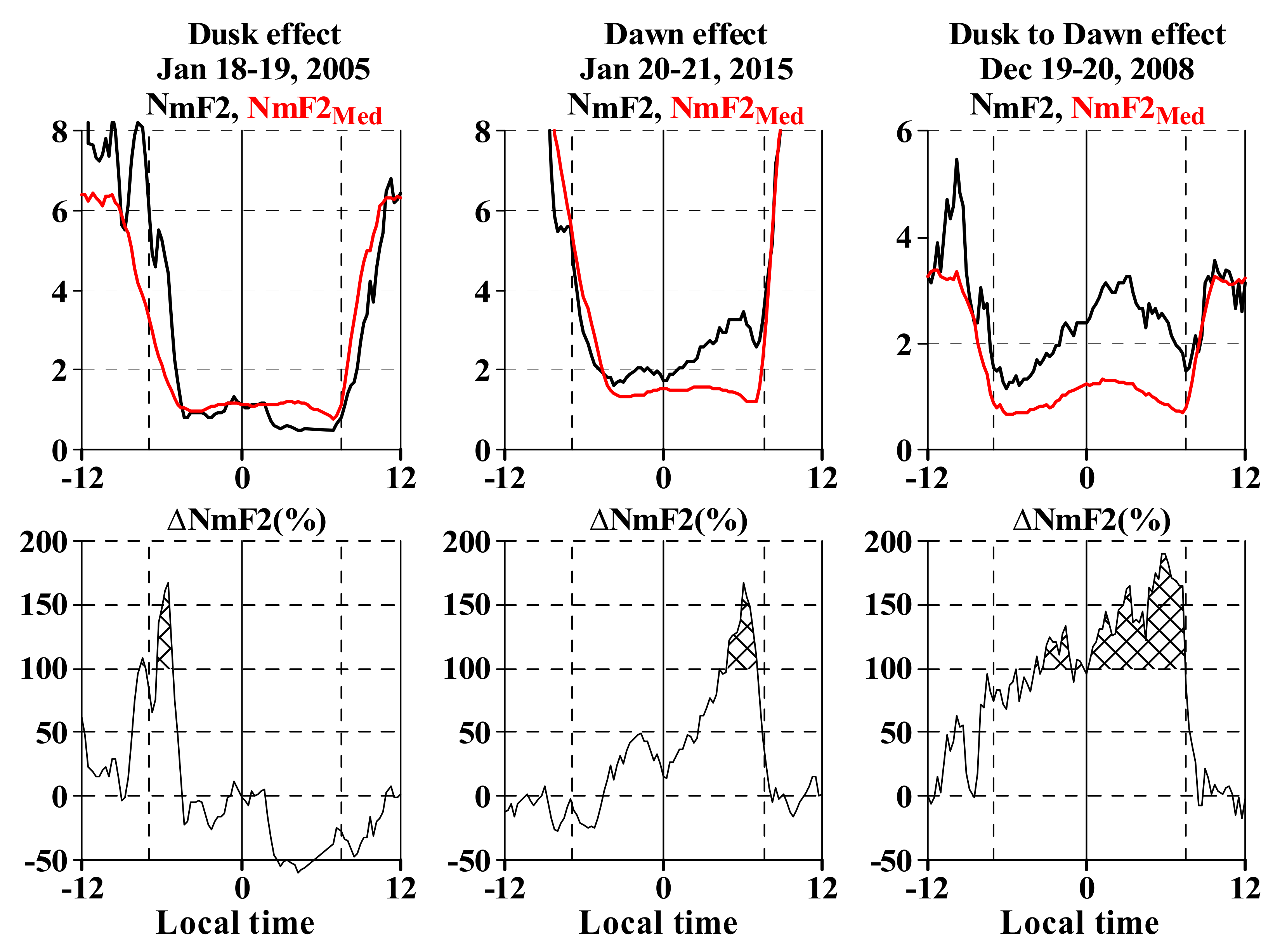
Figure 1 demonstrates three examples of extreme ionospheric disturbances over Irkutsk: the first type (first column) presents the case of near sunset disturbance (18–19 January 2005), the second type (second column) was related to a disturbance observed near dawn (20–21 January 2015), and the third type (third column) shows the case when a strong disturbance NmF2 (>100%) was observed during almost the entire night (19–20 December 2008).
The first type is known as the dusk effect [
29]. By analogy, we may call the second type the “dawn effect” and the third type “from dusk to dawn effect”. The third presented case demonstrates unique ionospheric disturbances when the winter nighttime NmF2 on 20 December 2008 was larger than the noontime NmF2 of the same day. The local time occurrence of all the observed extreme ionospheric disturbances is presented in
Section 3.1.
3.1. Morphology of Extreme Ionospheric Events
From the entire Irkutsk database (2003–2016) of the ΔNmF2 with 15 min resolution, we identified 98 data samples when ΔNmF2 exceeded 150%.
Figure 2 shows the local time distribution of these cases.
The local time distribution of extreme disturbances shows that they were observed either in the post-sunset period (0–6 h after sunset, ~83% of cases) or in the pre-sunrise period (0–4 h before dawn, ~17% of cases). In the post-midnight period (00–02 LT) and during the sunlight time (08–16 LT), the extreme cases were not observed. From the entire Kaliningrad database (2009–2016) of the ΔNmF2 with 1 h resolution, we identified only six cases of extreme disturbances by the criterion ΔNmF2 > 150%; four cases were the dusk effect, and two cases were the dawn effect. The difference between the Kaliningrad and Irkutsk statistics is discussed in
Section 4. The local time distribution of extreme NmF2 disturbances indicated that ΔNmF2 > 150% occurred only under nighttime conditions. Further analysis was carried out in terms of extreme ionospheric events: one event represented a night when the ΔNmF2 was greater than 150%. In total, the 2003–2016 Irkutsk database of the ΔNmF2 represented 25 extreme ionospheric events (on average 1.8 events per year), while the 2009–2016 Kaliningrad database of the ΔNmF2 gave six extreme ionospheric events (on average 0.75 events per year).
Figure 3 shows the seasonal distribution of the extreme ionospheric events from the Irkutsk database. As seen from
Figure 3, most of the events took place in January (10 events) and December (9 events), fewer in February (3 events) and November (2 events), and only one event in October. The diurnal-seasonal distribution shows that the most probable time of extreme events occurrence was the pre-dawn and post-sunset periods in December–January. On the one hand, this period corresponded to the highest ionospheric short-term variability according to the statistical analysis of the Irkutsk ionosonde data [
30]. On the other hand, this period corresponded to the lowest values of NmF2 in the regular diurnal-seasonal variations [
31]. Of the six Kaliningrad extreme events, three occurred in January and three in November, February, and March (one event for each month). Note that there were no extreme events at Irkutsk in March.
Figure 4 shows the year-by-year distribution of the extreme ionospheric events from the Irkutsk database. The year-by-year distribution of extreme events does not show a clear dependence on solar/geomagnetic activity in terms of yearly mean F10.7 and Ap values. For example, in the year of the highest geomagnetic activity (2003) one may see the same number of extreme events as at the solar/geomagnetic minimum (2009), while the largest number of extreme events was seen in 2005 at the declining phase of solar cycle 23. Thus, the morphological analysis showed that the extreme ionospheric disturbance was the nighttime phenomenon that occurred from late October to early March (mainly in December–January) and did not have a clear dependence on solar/geomagnetic activity in terms of yearly mean F10.7 and Ap values.
3.2. Relation of Extreme Ionospheric Events with SSWs
The dates of extreme ionospheric events were compared with the periods and dates of SSWs. The comparison showed that only two out of the 25 Irkutsk extreme ionospheric events occurred during SSWs. These were the major January-February SSWs of 2006 and 2009. We may also distinguish the extreme events of 31 December 2003 and 25 January 2004, which occurred five days before and seven days after the January 2004 SSW. In other cases, the dates of extreme ionospheric events and the dates of SSWs differed by 15 days or more. Thus, SSW cannot be considered as the main cause of the Irkutsk extreme ionospheric events. This fact does not mean the absence of SSW impact on the ionosphere. For example, the minor February 2016 SSW led to strong nighttime NmF2 disturbances, but the response amplitude was not extreme [
32].
The Kaliningrad extreme ionospheric events were more closely related to SSWs than the Irkutsk events: three out of six Kaliningrad extreme ionospheric events (i.e., half) occurred during SSWs. The Kaliningrad ionosonde dataset covers the 2009–2016 period, which included two major SSWs (January–February 2009 and January 2013) and one final SSW (March 2016); and all these SSWs were accompanied by extreme ionospheric events at Kaliningrad. In two cases of three, the extreme events occurred on the day of the SSW onset (the day of zonal mean zonal wind reversal), and in one case they occurred two days after the SSW onset. Unlike Irkutsk, SSW can be considered as one of the main causes of extreme Kaliningrad ionospheric events.
3.3. Relation of Extreme Ionospheric Events with SGSs
The dates of extreme ionospheric events were compared with the dates of SGSs. The comparison showed that 12 out of 25 (i.e., about half) Irkutsk extreme ionospheric events may be related to SGSs. Among the SGSs accompanied by Irkutsk extreme ionospheric events, we found four intense storms (Dst ≤ −100 nT) that included the well-known Halloween storm, the severe storm of 15 December 2006 associated with the long-duration positive storm effect [
33], the strong storm of 18 January 2005 associated with the extremely strong positive storm effect [
34], and the strong storm of 22 January 2004 associated with the strong positive storm effect at low latitudes around local sunset time [
35].
The SGS occurrence decreased greatly at the deep solar and geomagnetic minimum of cycle 23/24 compared to the declining phase of solar cycle 23. From January 2007 to February 2011 there were seven Irkutsk extreme ionospheric events, none of which were related to SGSs. In order to increase the set of storms, we reduced the criterion to −30 nT and considered small storms (−50 nT < Dst(Tmin) ≤ −30 nT). This increase in the storm set showed that three Irkutsk extreme ionospheric events may be related to the small storms. Of the two extreme ionospheric events that occurred during SSWs, one may be related to the moderate storm (SGS list) and the other one to the small storm. Finally, 15 out of 25 Irkutsk extreme ionospheric events may be related to SGSs, small storms, and/or SSWs; however 10 extreme events remained unexplained. In order to explain these 10 extreme events, we considered RGSs as potential sources of extreme ionospheric disturbances.
The comparison of Kaliningrad extreme events with the dates of SGSs and small storms showed that two out of six Kaliningrad extreme ionospheric events may be related to SGSs (moderate storms in both cases), one of which occurred during the final March SSW.
3.4. Relation of Extreme Ionospheric Events with RGSs
The dates of extreme ionospheric events were compared with the dates of RGSs. The comparison showed that 18 out of 25 (i.e., 72%) Irkutsk extreme ionospheric events and two out of six Kaliningrad extreme ionospheric events may be related to RGSs. The RGSs accompanied by the Irkutsk extreme events are partly included in the SGS list (6 out of 18) and partly supplement it (12 out of 18). The RGSs accompanied by the Kaliningrad extreme events are not included in the SGS list.
All storms accompanied by extreme ionospheric events were divided into storms driven by co-rotating interaction region (RGSs or CIR-storms) and storms driven by coronal mass ejection (CME-storms). As a result, the relation of extreme ionospheric events with geomagnetic and meteorological activity is as follows. At Irkutsk, 18 extreme events out of 25 may have been related to RGSs (one case also may be related to SSW); six extreme events out of 25 may have been related to CME storms (one case also may be related to SSW); and one extreme event out of 25 was related neither to storms nor SSWs. Thus, RGS may be considered the main cause of extreme ionospheric events at Irkutsk. At Kaliningrad, two extreme events may have been related to both SSWs and storms (both RGS and CME-storm); two extreme events may have been related to storms without SSWs (both RGS and CME-storm); one extreme event may have been related to SSW and without storms; and one extreme event was related neither to storms nor SSWs. Thus, the main cause of extreme ionospheric events at Kaliningrad is not clear. We may suppose that the contribution of SSWs and storms to producing extreme ionospheric events may be comparable.
Table 1 demonstrates the complete list of extreme ionospheric events and their potential sources for Irkutsk (2003–2016) and Kaliningrad (2009–2016) data.
Earlier (
Figure 4), we concluded that the year-by-year distribution of the Irkutsk extreme ionospheric events did not show a clear dependence on solar/geomagnetic activity in terms of yearly mean F10.7 and Ap values. Given that the extreme ionospheric event was mainly a winter phenomenon related to an RGS or CME-storm, we can revise the year-by-year variations. Instead of number of extreme events by year, we considered number of extreme events by winter: winter of a year is the period including the first 45 days of this year and the last 45 days of the previous year. Only two extreme ionospheric events out of 25 occurred outside the winter period (one related to the RGS and the other one to the CME-storm). Instead of yearly mean F10.7 and Ap values, we considered number of RGSs and SGSs by winter.
Figure 5 shows the results of the revision.
Three conclusions may be obtained from
Figure 5. The RGSs tightly covered the solar/geomagnetic minimum and were able to explain extreme ionospheric events during this period. The number of extreme ionospheric events at Irkutsk correlated with the number of RGSs at the declining phase of solar cycle 23 and solar/geomagnetic minimum, but the correlation decreased at the rising phase of solar cycle 24. From the total number of the events, we can estimate the probability of extreme events during RGS. Considering that 17 out of 23 extreme events could be related to RGS, the probability is ~0.12, i.e., on average, every 8th storm is accompanied by extreme ionospheric event. The reasons for this low probability are discussed in
Section 4.
4. Discussion
The analysis of extreme ionospheric events at Irkutsk showed that all events, except one, may have been related to geomagnetic storms, mainly to RGSs (18 cases out of 25) and partly to CME-storms (6 cases out of 25). The analysis of Kaliningrad events did not reveal the main cause of extreme ionospheric events: three out of six Kaliningrad extreme ionospheric events (i.e., half) occurred near SSW onsets, indicating that SSW may play a major role in the event occurrence; however, two out of six Kaliningrad events may have been related to storms without SSWs (both RGS and CME-storm).
The analysis raises the following open questions:
Why is not every RGS accompanied by extreme ionospheric disturbances?
The extreme ionospheric events at Kaliningrad have lower occurrence, higher sensitivity to SSWs, and lower sensitivity to RGSs compared to those at Irkutsk. What is the reason for the difference between the Kaliningrad and Irkutsk extreme ionospheric events?
What is an extreme ionospheric event related neither to storms nor SSWs?
What are the mechanisms for producing extreme ionospheric disturbances?
Typically, the recombination rate of O+ ions increases during geomagnetic storms due to an increase in the density of molecular nitrogen [
36,
37]. Cai et al. [
38] showed that ∑O/N2 depletion may be significant and long-lasting phenomena even under weak geomagnetic activity. The increase in the recombination rate results in a negative ionospheric storm (decrease in electron density) and reducing the positive ionospheric storm (increase in electron density). In our case, the increase in the recombination rate is the first factor that reduces the probability of the positive extreme disturbances in NmF2 during a storm. The lower the geomagnetic latitude is, the less the increase in the recombination rate under storm conditions [
36,
37,
38]. This may explain the lower occurrence and lower sensitivity to RGSs for extreme ionospheric events at Kaliningrad compared to those at Irkutsk (the geomagnetic latitude at Irkutsk is 11° lower than that at Kaliningrad). However, the higher sensitivity to SSWs for the Kaliningrad extreme ionospheric events is unclear.
Most of extreme ionospheric events occurred either in the post-sunset period or in the pre-sunrise period. This means that the time of the largest storm impact should be close to the local time of sunset or sunrise. The need for such a combination is the second factor that reduces the probability of the positive extreme disturbances in NmF2 during a storm. The third factor is an arbitrarily chosen threshold for identifying extreme events; lowering this threshold may increase the probability.
The Irkutsk extreme ionospheric event related neither to storms nor SSWs is the event shown in
Figure 1, and it is called as “from dusk to dawn effect”. Deminov et al. [
39] noted that such an extreme case in the ionosphere is very rare, and supposed that it could be caused by the superposition of the changes in thermospheric parameters and processes of interaction between the solar wind and magnetosphere, including the southwards rotation of the IMF. In our opinion, such cases require a separate analysis and a different definition of an extreme event. Instead of considering the extreme ΔNmF2 values, we may propose an analysis of the largest values of nighttime averaged disturbances.
Among the reasons causing extreme ionospheric events, the following mechanisms for producing extreme ionospheric disturbances can be considered. Buonsanto analysis [
29] of the dusk effect (large enhancement in electron density at middle latitudes in the evening hours) revealed three possible mechanisms: storm induced traveling atmospheric disturbances resulted in a convergence of plasma in to the peak density region, electric field induced advection of high-density plasma from lower latitudes, and neutral composition changes. Foster et al. [
1,
3,
6] highlighted the main role of the electric field for producing storm enhanced density: the penetration electric field redistributes the equatorial ionospheric plasma and forms the equatorial anomaly peaks at lower latitudes, whereas the polarization electric field at the dusk terminator redistributes the enhanced electron density further in both longitude and latitude. Another mechanism for producing strong positive nighttime NmF2 disturbances is associated with an increase in the downward plasmaspheric flux [
39,
40]. This process may be initiated by an increase in the peak height hmF2 due to thermospheric wind [
40] or by an increase in the plasmaspheric density due to the electric field induced plasma drift from a large volume geomagnetic field tube into one with a smaller volume [
39]. In our case, the extreme ionospheric disturbances near sunset or sunrise are most likely related to the electric field induced plasma drift from the sunlit side to the dark side; while the extreme ionospheric disturbances observed during almost the entire night are most likely related to the increase in the downward plasmaspheric flux.
Our analysis revealed that RGS may be considered as the main cause of extreme ionospheric events at Irkutsk. This fact prompts us to briefly discuss the role of RGSs (or CIR-storms) in ionospheric variability. Dmitriev et al. [
26], analyzing the statistics of ionospheric storms in the region of dayside equatorial ionization anomaly during RGSs, revealed the substantial enhancements of TEC within a few days after the storm onset and found the correlation of the TEC enhancements with the heliospheric and geomagnetic drivers. Chen et al. [
41], comparing the effects of CIR- and CME-induced geomagnetic activity on thermospheric densities and spacecraft orbits, showed that, in general, the effect of CIR storms on thermospheric density and satellite orbits is comparable to or even greater than that of CME storms. Cai et al. [
38] demonstrated that weak geomagnetic activity plays an important role in the variations of thermosphere composition during solar minimum “quiet” conditions: the ∑O/N2 depletion reached 30% of quiet time values during weak geomagnetic activity. Modeling of the thermospheric responses to geomagnetic storms for both solar maximum and minimum conditions showed that the decrease in electron densities should be greater at solar minimum than at solar maximum for equivalent storms at each part of the solar cycle [
42]. Buresova et al. [
28] compared ionospheric responses to the strong magnetic storms of January 2000 and October 2012 with those of the minor magnetic storms of January and November 2008 using digisonde measurements at middle latitude stations across European-African and American regions. The comparison showed that the ionospheric effects of CIR-related storms under extremely low solar activity conditions were comparable with the effects of strong CME-generated storms under higher solar activity conditions. Do these results mean that the ionospheric variability at the maximum (when CME-storms dominate) and minimum (when CIR-storms dominate) of geomagnetic activity are comparable with each other? The answer depends on the selected measure of ionospheric variability. The statistical analysis of ionospheric variability from the Irkutsk digisonde data [
30] showed that the nighttime variability and the short-term variability both for the day- and nighttime were comparable at the geomagnetic minimum (2009) and geomagnetic maximum (2003). However, at the same time, the long-term daytime variability showed a clear increase in the geomagnetic activity level and correlation with the annual mean of Ap-index.
We analyzed the behavior of the peak height (hmF2) during extreme ionospheric events (ΔNmF2 > 150%). Each case of ΔNmF2 exceeding 150% corresponded to some disturbance of hmF2 (absolute deviation of the observed value from the 27-day running median value).
Figure 6 shows the histogram of the percentage distribution of hmF2 disturbances (ΔhmF2) for extreme cases of ΔNmF2 > 150%.
The cases when extreme ΔNmF2 corresponded to large positive ΔhmF2 were rare events: ΔhmF2 exceeds 40 km only in ~5% of cases. The most probable case is near zero or slightly negative values: ΔhmF2 is in the range from −20 to 0 km in ~52% of cases. If the cause of extreme ΔNmF2 was vertical plasma drift due to neutral wind surge or disturbance of the eastward electric field, then correlated behavior would have occurred: large ΔNmF2 correspond to large ΔhmF2. Such cases do occur but as an exception. Therefore, we can conclude that neutral wind surges or eastward electric field disturbances are not the main cause of extreme ΔNmF2 occurrence. If the reason for extreme ΔNmF2 is horizontal plasma drift from the sunlit side to the dark one, then one would expect a decrease in hmF2 rather than an increase (on the sunlit side, hmF2 is lower than on the dark side). On the whole, the obtained distribution of ΔhmF2 fits into this hypothesis. If the cause of extreme ΔNmF2 is downward plasma drift (from the plasmasphere to the ionosphere) or a change in the neutral composition, then hmF2 disturbance can be both positive and negative. As a result, two conclusions can be drawn from the obtained distribution of ΔhmF2: (1) neutral wind surges or eastward electric field disturbances were not the main cause of extreme ΔNmF2; (2) the obtained distribution of ΔhmF2 did not contradict the hypothesis that the main cause of extreme ΔNmF2 was the horizontal plasma drift from the sunlit side to the dark one. Plasma fluxes from the plasmasphere to the ionosphere and changes in the neutral composition can also play an important role in producing extreme ionospheric disturbances.
5. Conclusions
With the long observation series at the Irkutsk (52° N, 104° E) and Kaliningrad (54° N, 20° E) ionosondes we obtained the datasets of ionospheric disturbances that were treated as relative deviations of the observed peak electron density values from their 27-day running median values. As the extreme disturbances, we considered cases when the disturbance was greater than 150%. As potential sources of extreme ionospheric disturbances, we considered sudden stratospheric warmings, geomagnetic storms by the criterion Dst ≤ −30 nT, and recurrent geomagnetic storms that did not necessarily satisfy the criterion for Dst.
The morphological study gave the following pattern. The extreme disturbances were observed either in the post-sunset period or in the pre-sunrise period. Further analysis was carried out in terms of extreme ionospheric events: one event represented a night when the disturbance was greater than 150%. In total, the 2003–2016 Irkutsk dataset gave 25 extreme ionospheric events (on average 1.8 events per year), while the 2009–2016 Kaliningrad dataset gave six extreme ionospheric events (on average 0.75 events per year). The seasonal distribution showed that most of the events took place in January and December, fewer in February and November, and only one event in October and March. The diurnal-seasonal distribution showed that the most probable time of extreme disturbances occurrence was the pre-dawn and post-sunset periods in December–January. The year-by-year distribution of extreme events did not reveal a clear dependence on solar/geomagnetic activity in terms of yearly mean F10.7 and Ap values but showed a correlation between the number of events and the number of recurrent geomagnetic storms.
The study of the relationship between extreme ionospheric events and manifestations of geomagnetic and meteorological activity revealed that about half of the extreme ionospheric events may have been related to geomagnetic storms by the criterion Dst ≤ −30 nT and/or sudden stratospheric warmings. Consideration of recurrent geomagnetic storms allowed us to find the sources of almost all extreme ionospheric events. The final relation of extreme ionospheric events to space weather events is as follows. Geomagnetic activity may be considered the main cause of extreme ionospheric events at Irkutsk (mainly associated with recurrent geomagnetic storms and partly with CME-storms); while the main cause of extreme ionospheric events at Kaliningrad is not clear (a comparable contribution of sudden stratospheric warmings and storms can be assumed). The extreme ionospheric events at Kaliningrad had lower occurrence, higher sensitivity to sudden stratospheric warmings, and lower sensitivity to recurrent geomagnetic storms compared to those at Irkutsk. This difference may be explained by the higher geomagnetic latitude of Kaliningrad and, consequently, by a larger increase in the recombination rate under storm conditions.


 ,
, 


