1. Introduction
Rainfall is undoubtedly one of the most significant natural phenomena that plays a key role in the natural life and habitat of the earth. However, excessive rainfall can trigger natural disasters that put millions of lives at serious risk. In Malaysia, the rainy season, also known as the Northeast Monsoon season, runs from November to January each year and contributes 60% of the annual rainfall in East Malaysia. Along the east coastline of Malaysia, states such as Kelantan and Terengganu receive very heavy rainfall with over 3500 mm of rainfall annually. Each subsequent rainfall event over the rainy season increases the discharge of rainfall. Since Malaysia often encounters such issues, hydrologists have studied the rainfall trend in Malaysia with an emphasis on extreme rainfall events [
1,
2,
3].
For instance, Malaysia experienced a massive flood in November of 2005. The flood hit various locations in Malaysia, including Kota Bharu, Kelantan. The disastrous event was described as the worst natural flood in history. Afterwards, in the years 2006, 2007, and 2008, heavy monsoonal rainfall again triggered major floods along the East Coast as well as in other parts of the country [
4]. The hardest-hit areas were again along the East Coast of Peninsular Malaysia in the states of Kelantan, Terengganu, and Pahang.
In hydrological studies, these events are known as torrential rainfall. The term torrential rainfall has been used to describe extreme rainfall exceeding the threshold of 60 mm/day based on the classification of rainfall intensity by the Department of Irrigation and Drainage, Malaysia (DID) [
5]. The East Coast region of Peninsular Malaysia often receives torrential rainfall during the Northeast Monsoon season. Due to this, several states located in the East Coast region face massive flooding every year. Climatologists or hydrologists could put this data to use to recommend additional measures to mitigate flood damage or to take precautions when flooding occurs [
6].
Over the last few decades, there has been abundant research on spatial and temporal rainfall as well as its effect on the catchment areas [
7]. The study of spatial and temporal rainfall has proved its importance in modeling and forecasting future rainfall patterns [
8]. The study of spatial and temporal rainfall in hydrology is comprised of two approaches: regression-based modeling and cluster-based modeling. Previous studies [
9,
10,
11] used regression-based modeling that generally aims to characterize the rainfall distribution patterns. With this approach, identifying spatial and temporal patterns of rainfall focuses on detecting trends rather than describing the regional characteristics of each pattern.
Nevertheless, studies related to cluster-based approaches in identifying spatial and temporal rainfall patterns aim to quantify the characteristics of a set of observations that fit into the same group, meaning that the patterns are similarly highly structured [
12]. In addition, this approach is perceived as an efficient statistical tool in handling tasks such as grouping each region and identifying time periods based on the groups to reflect the occurrence of rainfall events.
Cluster analysis is often used to identify the rainfall patterns. Classical clustering methods, such as k-means clustering, require certain assumptions that contradict the characteristics of rainfall by dividing the database of rainfall patterns into clusters with the assumption that every weather pattern exclusively belongs to only one specific cluster. Using classical clustering, each day is respectively assigned to only one cluster [
13]. These assumptions may not reflect reality, since one day could include several different types of weather at different stations.
Researchers have proven the superiority of using the Fuzzy C-means (FCM) as opposed to other clustering algorithms [
14,
15]. As a result, several clusters can belong to one data point when the Fuzzy C-means are used. The distance between the data point and the cluster center is used to assign the membership of each data point. It is more feasible to use a cluster located near a cluster center for particular sets of data. For instance, a study [
16,
17,
18] proved that the FCM were very stable compared to other clustering algorithms, even when outliers and overlapped variables were present. The FCM algorithm incorporates noise, outliers, and non-uniform mass distributions to make the method applicable to data with unequal cluster sizes [
19]. The FCM algorithm has proven its capability in handling datasets contaminated by noise and outliers. Previous researchers have applied this algorithm in various areas, including image processing [
20,
21,
22].
Aside from traditional cluster algorithms, the usage of PCA has proven to be effective in identifying the number of clusters and improving cluster accuracy. Previous studies [
23,
24] have demonstrated the capability and applicability of PCA in identifying the number of clusters for rainfall patterns. However, the classical PCA can be insensitive to outliers, as it assigns equal weights to each set of observations [
25]. Hence, applying the classical PCA may affect overall cluster partitions of the rainfall patterns.
In clustering torrential rainfall patterns of the East Coast of Peninsular Malaysia, a long time series of observed rainfall data trends is needed. This is because the amount of rainfall for tropic regions does not vary significantly from day to day as compared to daily rainfall averages in four-season regions [
12]. However, high-dimensional datasets tend to contain many irrelevant features that will affect the accuracy of the results [
26]. Therefore, feature selection is considered to be an essential procedure in the processing of high-dimensional data [
27]. There are few widely used dimensionality reduction methods that deal with spatial and temporal datasets. For instance, researchers [
28] applied discriminant analysis (DA) in finding the relation between rainfall and landsides, while others [
29] demonstrated the capability of non-linear principal component analysis in dealing with a climate dataset. On the other hand, many other researchers [
30,
31,
32] have applied PCA in identifying the rainfall patterns for climate analysis.
The aims of this study are twofold: to propose statistical modeling using a combination of Robust PCA and the Fuzzy C-Means clustering method and to validate the outcome of the proposed model against the classical PCA in terms of the quality of internal and external clustering methods based on clustering validity indices. The proposed model is expected to improve the cluster partitions by using effective inputs from significant underlying patterns from the torrential dataset. It is anticipated to counter the shortcomings of the clustering approach for determining rainfall patterns on the East Coast of Peninsular Malaysia. Consequently, a robust measure of location and scale in the PCA was incorporated using Tukey’s biweight correlation to downweight observations that were far from the data center and resistant to outlying observations due to their characteristics. The Fuzzy C-Means method exhibited the capability for overlapping data set in cluster partitions based on the membership level.
3. Methodology
3.1. Principal Component Analysis (PCA)
By retaining most of the original variability in the data, PCA is designed to reduce the dimensions of large data to a lower dimension [
34]. This is achieved by converting a set of observations of possibly correlated variables into a set of linearly uncorrelated principal components. The first principal components account for much of the original data’s variability. Then each successive component accounts for the remaining variation subject to the previous component being uncorrelated.
When PCA is applied, the covariance or correlation matrix, derived from the data matrix is used to calculate its eigenvalues and eigenvectors [
35]. In this study, the eigenvectors and eigenvalues were calculated from the correlation matrix to find the components that best explain variance in the data.
For the extraction of the number of components, it is recommended to take at least 70% of the cumulative percentage of total variation as a benchmark to cut off the eigenvalues in the large data sets [
36]. The reduced matrix is the component matrix of eigenvector “loadings” that defines the new variables consisting of the linear transformation of the original variables maximizing the variance in the new. The steps involved in the PCA algorithm are shown in
Figure 2.
3.2. Pearson Correlation Matrix
In applications of hydrology and climatology, the Pearson correlation is typically used in the PCA for calculating the eigenvectors and eigenvalues [
37,
38]. The Pearson correlation coefficient between two variables is defined as the covariance of the two variables divided by the product of their standard deviations. Typically, the Pearson correlation is used to measure the distance (or similarities) before implementing a clustering algorithm. The Pearson correlation coefficient between two vectors of observations is as follows:
where
and
refer to the vectors of observations in matrix data
with
observations, with
and
referring to the mean of the vectors.
3.3. Tukey’s Biweight Correlation
Tukey’s biweight correlation is based on Tukey’s biweight function that relies on the M-estimator used in robust correlation estimates. The M-estimator has a derivative function
which determines the weight assigned to the observations in the data set. It has the ability to down-weight observations to reflect their influence from the mean of the data [
39].
Let matrix
be the rainfall data in the east coast of Peninsular Malaysia comprising
observations (i.e., rainfall days) defined by
variables (i.e., rainfall stations) denoted by the
matrix
, whose generic element is
. After that, the data was standardized using median and mean absolute deviation (MAD). This was conducted to prevent any masking or swamping effects [
40]. The standardization of
is computed as follows
such that
refer to elements in the input matrix,
.
Let
denote an
matrix
, in which its generic element is
comprising
observations (i.e., rainfall days) described by
variables (i.e., rainfall stations). Let
be the valuation that minimizes
where
is described as the objective function and the M-estimator of location
). Consequently,
where
denotes the derivative of
with respect to
which is used to simplify the calculation of the M-estimator by computing a value of
.
To calculate
and
, it is mandatory to measure the observation and choose some estimators of matrix, called
, and also a function of each element,
) of matrix
. Hence, the observations are converted to
where
is the location matrix,
is the shape matrix, and
is the positive constant, which is an equally tuning constant. To simplify the interpretation, the algorithm is shown in one dimension as:
Equation (6) substituted in Equations (3) and (4) to obtain
and
where
and
that solve Equation (7) are the consequential M-estimates of location and shape, correspondingly.
The derivative function is derived as follows:
It can be seen that if
is large enough, then
reduces to zero. One of the important aspects of measuring the resistance to outlying data values of M-estimators is its breakdown point. According to the study, the breakdown point is used in measuring their resistance to outlying data values [
41]. However, in the PCA-based Tukey’s biweight correlation, the breakdown point is used to determine the ideal number of components to extract. Adjustments of the breakdown point will have an effect in determining the number of components to obtain using the PCA method [
12]. This study tested the performance of the biweight correlation under various point changes in order to determine the number of components to extract from the PCA in order to identify the pattern of torrential rainfall. In this study, Tukey’s biweight with breakdown points at 0.2, 0.4, 0.6, and 0.8 are compared.
The biweight estimate of correlation is produced by first calculating the location estimate
and then updating the shape estimate,
. The
element of
, i.e.,
acts as a robust estimate of the covariance between the two vectors,
and
. The biweight correlation of these two vectors is calculated as follows:
with
where
is a location vector and
is a shape matrix such that
Thus, a PCA-based Tukey’s biweight correlation is more likely to produce a better cluster partition that is more resistant to outlying values than the Pearson correlation in PCA.
3.4. K-Means
This algorithm consists of two separate phases; the first step is to randomly select
k objects, each of which initially represents a cluster mean or center. The next phase is to assign each data point
to the nearest cluster center. The Euclidean distance method is generally used to determine the distance
between each data point
and centroid
as shown below:
When all the data points are assigned to each of the clusters, the cluster centroid is recalculated. A schematic procedure of the k-means method is also presented below; the k-means clustering algorithm works as follows:
Step 1: Randomly choose objects from a data set as an initial cluster centroid.
Step 2: Calculate the distance between each data point and assign each item to the cluster which has the closest centroid. Recalculate the cluster centroid for each cluster until the convergence criteria is reached.
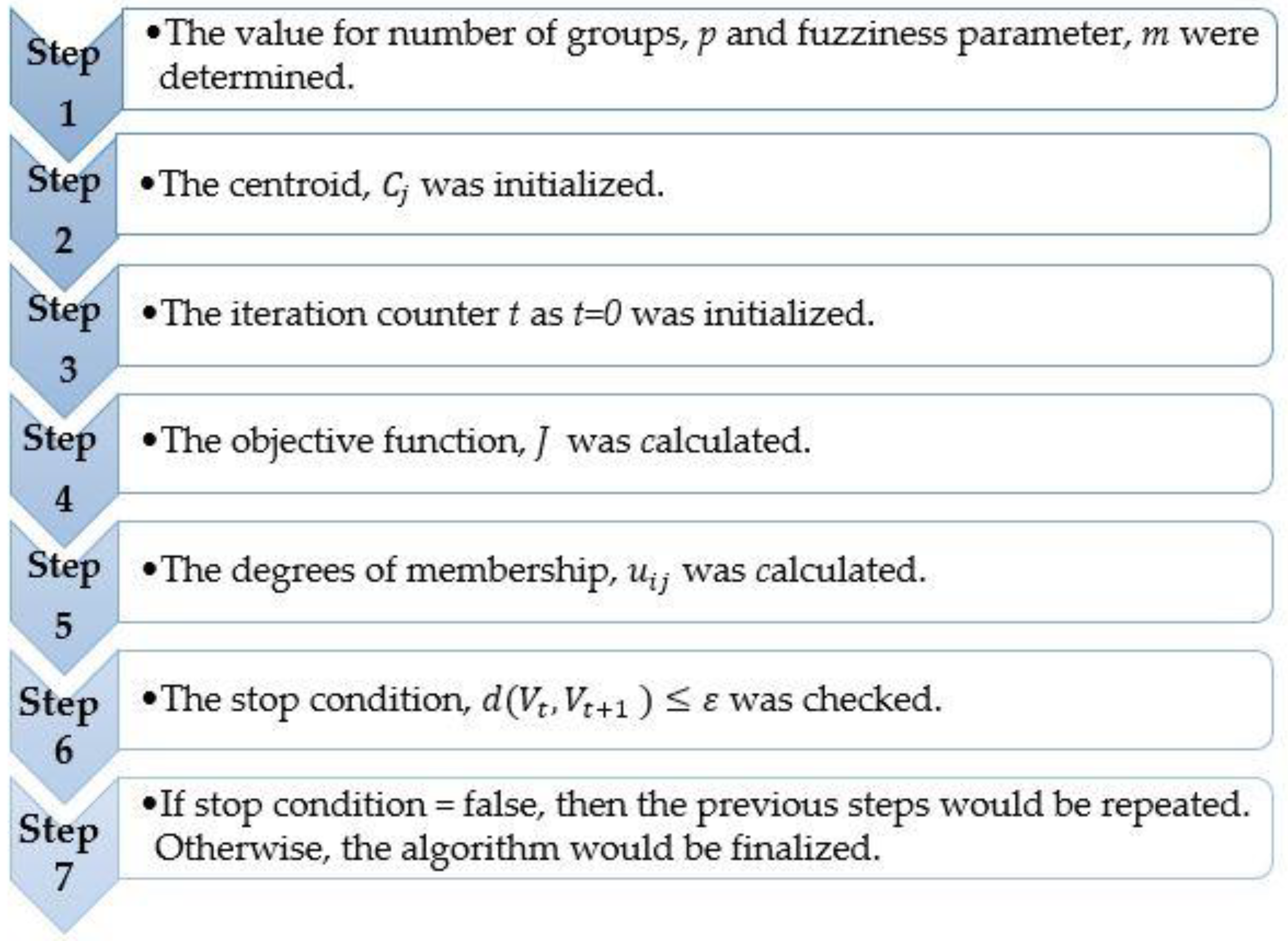
3.5. Fuzzy C-Means Clustering (FCM)
Bezdek [
42] introduced a clustering approach, FCM, which is widely used in solving the problems connected with feature analysis, clustering, and classifiers. Generally, fuzzy clustering refers to assigning values to membership levels and using them to assign data elements to one or more clusters. When using k-means clustering algorithms, each pattern belongs to only one cluster. However, fuzzy clustering goes a step further and assigns or associates every pattern present in an image to every cluster of image data using a membership function.
The clusters in FCM are formed according to the distance between data points and the cluster centers formed. As compared to K-means, FCM clustering is well performed in that it allows the data to belong to more than one cluster [
43,
44,
45]. A dataset is grouped into
p clusters with every data point in the dataset related to every cluster; each data point that lies close to the center will have a high degree of connection to that cluster while another point which lies far from the center of a cluster will have a low degree of connection to that cluster [
46].
The FCM approach uses a fuzzy membership function that assigns a membership degree to each class. FCM splits the dataset
X into c fuzzy clusters. This algorithm holds that every object belongs to a specific cluster with various degrees of membership, while a cluster would be considered as a fuzzy subset on the dataset. FCM finds the partition that minimizes the objective function using the algorithm below [
47]:
where
n is the number of data;
p is the number of clusters;
is the degree of relevance of the sample
to the
j-th cluster;
is a measure of fuzziness that determines how membership between fuzzy clusters is shared;
d is the Euclidean distance between
and
;
is the data vector, with
i = 1, 2, …,
n, which signifies a data attribute; and
is the center of fuzzy clustering.
The FCM method relies on the fuzziness parameter m, and it works well when
m (1.5, 2.5) [
48]. In this study, the fuzziness parameter applied is
m = 2 as a default from the package that has been used. The quadratic total of the weighed distances from the samples to the cluster centroid in every cluster is known as the objective function [
49]. The objective function,
J is minimized, and the membership degrees,
are produced as the following formula:
where
can be obtained from:
In the interval (0, 1), the degrees of membership,
represent the probabilities that could be generated by a uniform distribution [
50,
51]. The clustering is modified at each iteration as the steps involved in the
Figure 3 shown below:
3.6. Proposed Statistical Modeling of RPCA-FCM
Robust PCA (RPCA) which is PCA based Tukey’s biweight correlation, is used to overcome the problems that affect cluster partitions and generate extremely unbalanced clusters in a high-dimensional space. RPCA is the robust version of classical PCA where the Pearson correlation is replaced with Tukey’s biweight correlation. This solves the issue of the number of clusters obtained by using classical PCA where the Pearson correlation assigns equal weight to the outliers. Outliers in hydrological data are potentially gained from various mechanism of physical phenomenon or from errors occurring during the measuring process. Additionally, outliers could be carrying substantial information about irregular conditions of hydrologic phenomenon. While Tukey’s biweight correlation is capable of assigning the weightage to the outliers in order to obtain the various number of clusters for the dataset used. To avoid any masking or swamping effects, the original data matrix is standardized using a robust location and scale estimator before proceeding. The reduced data set is then applied to the K-means cluster analysis to obtain the cluster partitions. The K-means method requires specifying the number of clusters before the algorithm is applied. To overcome this problem, the Calinski–Harabasz Index [
52] is used as a measure to determine the optimal number of cluster partitions for the input data. Lastly, the steps are continued by combining the FCM to allow each element in the data to belong to more than one cluster partition. This is due to the drawback of K-means clustering where the element in the data is only allowed to belong to one and only one cluster.
The steps involved in the proposed model are presented in
Figure 4 and the flowchart of the developed RPCA-FCM model is illustrated in
Figure 5.
3.7. Clustering Validity and Model Validation
The use of validity indices is important in order to contrast the clustering algorithms and compare the performance of clusters in terms of compactness and connectedness. Hence, the validation of the clustering results is a base for the clustering process. In this study, all of the external and internal criteria were used to calculate the quality of the clustering findings using two separate approaches in the correlation matrix.
Internal clustering validation uses internal information from the clustering process to assess the decency of a clustering structure. It can also be employed for guesstimating the number of clusters and suitable clustering algorithms. In this study, the silhouette index is used to reflect the compactness, connectedness, and separation of the cluster partitions to assess the quality of the clustering findings. The silhouette width is the average of each observation’s silhouette value. This technique finds the silhouette width for each single data point, the average silhouette width for every cluster, and the overall average silhouette width for the overall data set [
53]. The largest overall average silhouette width indicates the best clustering. Therefore, the number of clusters with maximized overall average silhouette width is considered the optimal number of the clusters. It can be concluded that the silhouette value measures the degree of confidence in a clustering study and lies in the interval (−1, 1), with well-clustered observations showing values near 1 and poorly clustered observations having values near −1.
The external criteria tested whether the points of the data set were randomly structured. There were many external quality indices and this study focused on the Rand index as a means of validating the clustering results. This index was calculated by determining the fraction of properly classified data points to every data point. The derivation of the Rand index has been described in previous studies [
54]. The ranges of the Rand index are between 0 and 1 where the value near 0 indicates that the pair is organized similarly under both clusterings, and the value approximate to 1 shows identical clustering.
The effectiveness of the properly identified clusters is shown by the following validity measures: partition coefficient, partition entropy, the fuzzy silhouette index, and the modified partition coefficient [
55,
56].
Based on the fuzzy partition matrix, the partition coefficient (PC) measures the degree of the fuzzy division of the clusters, as well as the quality of the partition; the larger its value, the better the partition results. Using the fuzzy partition matrix, the partition entropy (PE) measures the fuzzy degree of the final divided cluster, and the smaller its value, the better the partition. Meanwhile, the modified partition coefficient (MPC) decreases the monotonic tendency and the maximum value is shown at the best clustering of a given data set. The fuzzy silhouette index (FSI) is ideal for showing the maximum number of clusters so that the index takes the maximum value.
3.8. Monte Carlo Simulation
In order to assess the performance of the proposed model (RPCA-FCM), several sets of simulated data matrices generated by the Monte Carlo simulation were used to illustrate the methods described in
Section 3.6. These simulated data matrices were generated to mimic the real data and to follow the pattern of the original torrential rainfall data from East Coast Peninsular Malaysia. The purpose of using simulation is to determine an appropriate breakdown point and to evaluate the performance of the RPCA-FCM against the classical PCA in the analysis of identifying spatial cluster torrential rainfall patterns in East Coast Peninsular Malaysia.
The Monte Carlo simulation is capable of testing the performance of the normal and non-normal distribution of data [
57]. During the process, values are sampled at random from the input probability distributions. A sample is defined as a collection of samples. The outcome is reported from each sample. The Monte Carlo simulation is conducted through hundreds of iterations in order to obtain the optimal outcome.
The distribution is obtained for the creation of a
n ×
p matrix with
n = 175 and
p = 30 to reflect 175 torrential rainfall days and 30 rainfall stations correspondingly, from the original torrential rainfall data collected over 32 years from East Coast Peninsular Malaysia. All of the data produced shows values of about 60 and above, representing the torrential rainfall threshold of 60 mm/day. The standard algorithm of the Monte Carlo Simulation was illustrated in
Figure 6 [
58].
Every set of the produced data was further applied to two approaches that are either classical PCA or RPCA. From both approaches, the results were then contrasted based on the cluster partition, the number of components, and the validity measure of the original datasets.
4. Results and Discussion
4.1. Descriptive Analysis
Data preparation is one of the vital steps before proceeding with the analysis; it involves screening, evaluating, selecting records, and reducing the number of variables to a manageable range. A brief overview of the torrential rainfall data on the study area is provided in
Table 2 including descriptive statistics such as mean, standard deviation, and skewness.
All the stations give positive skewness with value 6.83. The results illustrated that the shape of rainfall distribution for the 48 stations is skewed because the values of the skewness are far from zero. Based on the data, it is likely that daily torrential rainfall does not originate from a normal population. Meanwhile, the kurtosis has the value of 139.47, indicating that the data has heavier tails compared to a normal distribution.
Table 2 shows that the average mean and average standard deviation of daily torrential rainfall amounts in East Coast Peninsular Malaysia are 7.78 and 17.80, respectively. Typically, the average coefficient of variation for the 48 rainfall stations is quite small, with the value of 2.29, exhibiting that the data have distributed evenly.
4.2. Choice of Breakdown Point for RPCA
The breakdown point is a significant element in the M-estimator for its tolerance towards the outlying data values. This study analyzed the choices of the breakdown point for
r = 0.2,
r = 0.4,
r = 0.6, and
r = 0.8.
Table 3 visualizes how the choice of the breakdown point affected the number of extracting components, as well as the clusters, in this approach.
From
Table 3, choosing
r = 0.2 was not suitable for this dataset where the highest internal validity measured at 90% cumulative percentage of variation while the highest value of the Rand index was at 70% cumulative percentage of variation. However, 60% to 70% of the cumulative percentage of variation obtained undefined the value for the silhouette index. This shows that
r = 0.2 is an unstable breakdown point for this dataset. While from
Table 3, it could be clearly seen that
r = 0.6 and
r = 0.8 can also be concluded as unstable breakdown points for RPCA. Based on the internal validity, the silhouette index, NA, was obtained for 60% to 85% cumulative percentage of variation used. In addition, the number of components to extract in both breakdown points was too small, affecting the validation measure of the clusters. However, it was impossible to increase the cumulative percentage of variation with the aim of increasing the number of components to extract. This is because higher cumulative percentage is defined as higher noise in the data. It is clearly proven that the cutoff for the breakdown point at
r = 0.6 and
r = 0.8 were not suitable for this dataset. Based on
Table 3, 90% cumulative percentage of variation obtained well-performed internal and external validity measures. However, the clusters obtained for the 90% cumulative percentage contained two clusters that were not a suitable cluster identifications for the rainfall study. The number of components to retain for 90% was also the highest (36 components) compared to other cumulative percentages of variation. Especially in hydrological study, if excessive components were extracted, it would show the insignificant variations of low frequency or spatial scale. Due to this fact, the 85% of cumulative percentage of variation using the breakdown point,
r = 0.4 was focused on in this study to improve the performance of the clustering.
It can be concluded that the best selection of the breakdown point for RPCA is
r = 0.4. This result is supported by previous researchers [
12,
41] who agreed that the breakdown point of
r = 0.4 offered a good balance to extract the best number of components since it retains only sufficient outstanding components.
The time consumed in calculating the validity index for the validity measure with a higher number of components takes a longer time compared to lower number of components. There is a limitation, as high-end computers with faster processing speeds are needed to acquire reliable and accurate results. The results can only be generated with the help of high-end computers and the application of machine learning methods that can improve the speed and accuracy of the test. In this study, we also found that extracting too low a number of components also affected the calculation for obtaining the validity measures of the clusters. This basically refers to a number of fewer than 10 components. In fact, the results that came out as NA for the number of components was less than 10. Hence, choosing the most accurate breakdown point is very important in using RPCA.
Based on the internal validity, the silhouette index, NA, was obtained for 60% to 85% cumulative percentage of variation used. Based on
Table 3, 90% cumulative percentage of variation obtained the well-performed internal and external validity measures. In contrast, the clusters obtained at 90% cumulative percentage were two clusters which were not suitable for the rainfall study since they mask the true structure of the data. The number of components to retain for 90% was also the highest, which was 36 components, compared to other accumulative percentages of variation. Especially in hydrological study, if excessive components were extracted, it would show the insignificant variations of low frequency or spatial scale. Due to that, 85% of cumulative percentage of variation in which the breakdown point,
r = 0.4 was focused on in this study to improve the performance of the clustering.
4.3. Evaluating Performance of Classical PCA against RPCA
From
Table 4, it shows that in order to obtain at least 60% of the total percentage of variance in contrast to the classical PCA, RPCA required less components to be extracted. Fourteen components were retained using RPCA as compared to the classical PCA, which required 30 components at 70% cumulative percentage of variation. This reflects the results of the number of components in each level of cumulative percentage of variation in which RPCA required a smaller number of components to extract compared to the classical PCA. However, the selection of excessively high cumulative percentages of variation was not a good cutoff for the number of principal components in identifying the rainfall patterns. This is due the fact that extracting a higher cumulative percentage of variation results in a higher number of components to retain. Inclusion of too many principal components inflates the importance of outlier, and the results become unsatisfactory in identifying the rainfall patterns [
25].
In terms of cluster partitions,
Figure 7 also shows that in contrast to the classical PCA, RPCA is more sensitive to the number of clusters according to the number of components retained. At 60% of cumulative percentage, RPCA resulted in the highest number of clusters (seven clusters) compared to the classical PCA. The number of cluster partitions becomes stabilized at 65% to 85% cumulative percentage of the variation of the data (four clusters). However, the resulting number of clusters was maintained as the classical PCA when obtained at more than 85% cumulative percentage of variance. Moreover, the number of clusters using the classical PCA appeared to stabilize at just two clusters, despite the cumulative percentage of variation employed.
This is due to the fact that the detection and treatment of the outliers in these observations is less effective when employing the Pearson correlation in the classical PCA because of its vulnerability towards the outliers. Additionally, the Pearson correlation in PCA assigns equal weight to each pair of observations. This would reduce the efficiency of the data due to the fact that the outliers undoubtedly stick out, causing information in the observation to be weakened. As a result, this correlation becomes ineffective in detecting the outliers.
In hydrological studies, particularly in identifying rainfall patterns, it is more reasonable to obtain more than two cluster partitions to explain various types of rainfall patterns. This shows that RPCA is capable of downweighting the outliers closer to the center as it helps in obtaining differentiated numbers of clusters compared to using the classical PCA.
4.4. Validity Measures of Clusters
Table 5 illustrates that the RPCA shows the relatively highest silhouette index with approaching 1 (0.9442) while the classical PCA obtained the smallest silhouette index at 0.6047. Similarly, RPCA also obtained a higher value of Rand index compared to the classical PCA. Therefore, from the clustering results, it can be concluded that RPCA correlation is more efficient in clustering hydrological data, especially for clustering the rainfall data of tropic regions.
4.5. Validity Measures of RPCA-FCM
The clusters obtained from the RPCA correlation were maintained as four optimal clusters. These clusters were then validated using the fuzzy silhouette index (FSI), partition entropy (PE), the partition coefficient (PC) and the modified partition coefficient (MPC) as shown in
Table 6. As a guideline, the smallest value of PE with the largest value of FSI, PC, and MPC represents a well-clustered partition.
From
Table 6, it can be seen that RPCA-FCM obtained the largest value of FSI, PC, and MPC with the lowest value of PE, while the combination of classical PCA with FCM obtained poor results. This result shows that the proposed statistical modeling, RPCA-FCM, performed well in clustering the torrential rainfall patterns of East Coast of Peninsular Malaysia compared to the classical procedure.
4.6. Evaluating the Performance of Proposed Models Based on Simulation Results
The data that mimicked the original dataset was then generated using the Monte Carlo simulation. In
Table 7, similar results were shown with the original data where the classical PCA required a greater number of components to extract in order to achieve at least 60% of the cumulative percentage of variation compared to the RPCA. For example, seven components were retained in the RPCA as compared to the classical PCA which required 28 components at 60% cumulative percentage of variation. This reflected the results obtained from the original data where RPCA required a smaller number of components to extract.
In terms of the number of clusters obtained, it can be seen that in contrast to the classical PCA, RPCA was more sensitive to the number of clusters according to the number of components retained. RPCA also showed similar results similar to the original data, whereas the classical PCA appeared to stabilize at only two clusters regardless of the cumulative percentage of variation used while the RPCA showed differentiating patterns of the number of clusters obtained.
Table 8 illustrates that RPCA showed a relatively higher silhouette index against the classical PCA. On the other hand, the classical PCA obtained a lower Rand index compared to the RPCA, proving that the RPCA is more well-clustered.
The analysis was then continued by using 85% cumulative percentage of variation for the simulated data in the FCM clustering. From
Table 9, the classical PCA combined with FCM obtained smaller values of FSI, PC, and MPC compared to RPCA combined with FCM. It also showed a higher value of partition entropy at 0.4419 compared to RPCA combined with FCM, which obtained a smaller value of 0.4126. This result shows the same results as implied by the original dataset where the proposed statistical modeling, RPCA-FCM, performed well compared to the classical PCA in clustering the torrential rainfall patterns of East Coast Peninsular Malaysia.
4.7. Description of Clustering of Rainfall Patterns
Using the results of the proposed statistical model RPCA coupled with FCM, four clusters were obtained. The clusters were then analyzed in order complete the cluster mapping.
As shown in
Figure 8, the pattern of torrential rainfall on the East Coast of Peninsular Malaysia is divided into daily torrential rainfall amounts from RP1 through RP4. As we compare the four clusters presented, it can be seen that the distinction between the torrential rainfall patterns were quite evident and that each pattern represented a different distribution of the rainfall. In each torrential rainfall patterns, there were distinct locations that were especially affected by the torrential rainfall. The highest rainfall recorded with an average amount of 229–238 mm.
Figure 8e shows the main torrential rainfall stations after filtering out days with rainfall more than 60 mm for at least 1.5% of the total number of stations.
Figure 8a refers to RP1, or generally exhibited moderate torrential rainfall, in the entire regions of Kelantan, Pahang, and Terengganu with an average amount of 85–117 mm where the highest percentage of days associated in this pattern was 40% of the torrential days over 32 years. The maximum average of torrential rainfall for RP1 occurred at Setor JPS KT (E1) in Terengganu with the record of 117.71 mm/day.
Figure 8b refers to RP2, or light torrential rainfall within the range of 81–101 mm throughout the whole region. The second-highest percentage of days associated in this pattern was 35.4% of torrential days over 32 years. Kg. Unchang (E20) recorded the maximum average of torrential rainfall at 100.06 mm/day.
Figure 8c refers to RP3, characterized as extreme torrential rainfall, since it generally represents heavy rainfall with an average amount of 76–238 mm in most regions. The maximum average torrential rainfall in RP3 is 237.80 mm/day at (E7). RP3 was associated with the lowest days of torrential days at 5.7%.
RP4 as referred to in
Figure 8d represents intense torrential rainfall with an average amount of torrential rainfall of 85–166 mm. This rainfall pattern was associated with 18.9% of torrential days over 32 years. It contributed to the second-highest maximum average of torrential rainfall of 165.8 mm, measured at Kg. Menerong (E4).
These results shows that the eastern areas are strongly affected by the Northeast Monsoon season that brings torrential rainfall to the East Coast regions from November until February. Therefore, the eastern part of Peninsular Malaysia is considered the wettest area during the Northeast Monsoon season. In particular, a maximum intensity is clearly distinguishable on the windward side of the mountain range. A large intensity gradient is observed across the mountain range, where greater values are recorded on the windward side of the mountain range and lesser values on its leeward side. The mountain range located in the center of the country forces the winds to rise and the rising air cools and condenses, resulting in heavy rains. The increased of intensity observed in October all across the peninsula may be attributable to the equatorward migration of another broad area of convergence. Intensity values are also greater in October than in April/May due to the fact that the convergence is smaller in the latter months than in the former. In spite of the fact that the intensity all across the peninsula increases in October, the same pattern prevails with larger values on the windward side of the mountain range and lesser values on its leeward side.


 ,
, 


