Article

A Climatological Study of the Mechanisms Controlling the Seasonal Meridional Migration of the Atlantic Warm Pool in an OGCM

1
Laboratoire de Physique de l’Atmosphère et de l’Océan Siméon Fongang (LPAO-SF/ESP/UCAD), Dakar 10200, Senegal
2
Laboratoire d’Océanographie et du Climat: Expérimentations et Approches Numériques (LOCEAN/UPMC), 75252 Paris, France
3
Laboratoire des Sciences de l’Atmosphère et des Océans (LSAO/UGB), Saint-Louis 234, Senegal
*
Author to whom correspondence should be addressed.
Atmosphere 2021, 12(9), 1224; https://doi.org/10.3390/atmos12091224
Submission received: 10 February 2021 / Revised: 20 June 2021 / Accepted: 26 June 2021 / Published: 18 September 2021
(This article belongs to the Special Issue Tropical Atlantic Variability)

Abstract

:
The tropical Atlantic Warm Pool is one of the main drivers of the marine intertropical convergence zone and the associated coastal Northeast Brazilian and West-African monsoons. Its meridional displacement is driven by the solar cycle, modulated by the atmosphere and ocean interactions, whose nature and respective proportions are still poorly understood. This paper presents a climatological study of the upper ocean and lower atmosphere contributions to the warm pool seasonal migration, using an Ocean General Circulation Model (OGCM). First, we provide quantitative, albeit simple, pieces of evidence on how the large amplitude of migration in the west, compared to the east, is mainly due to the strong east–west contrast of the background meridional SST gradient intensities, which is maintained by equatorial and eastern tropical upwellings. Our main results consist first in identifying a diagnostic equation for the migration speed of the two meridional boundary isotherms of the Warm Pool, expressed in terms of the various mixed-layer heat fluxes. We then evidence and quantify how, in general, the migration is forced by air–sea fluxes, and damped by ocean circulation. However, remarkable controls by the ocean are identified in some specific regions. In particular, in the northwestern part of the Warm Pool, characterized by a large temperature inversion area, the boreal spring northward movement speed depends on the restitution of the solar heating by the thermocline. Additionally, over the southern part of the Warm Pool, our study quantifies the key role of the equatorial upwelling, which, depending on the longitude, significantly accelerates or slows down the summer poleward migration.

1. Introduction

The Inter-Tropical Convergence Zone (ITCZ) is a band of deep atmospheric convection [1,2] which can also be defined as a region of heavy precipitation on-time average [3], produced by the convergence of the Trade winds [4,5] and by intense solar heating [6]. In tropical oceans, the warmest waters are generally found under regions with the most active convection [7,8]. The ITCZ is indeed coupled to the distribution of Sea Surface Temperatures (SSTs), with deep atmospheric convection favored by warm SSTs [9,10,11,12]. This has been confirmed numerically by [13], who showed that ITCZ migration is blocked in boreal spring when the cold tongue is prevented from developing. A common definition of the Warm Pool (WP) relies on the simple concept of an SST threshold value associated with deep convection. Some authors choose 27 °C [12,14,15], others 28 or 28.5 °C [16,17,18,19], and we will retain the first value for the boundaries of the tropical Atlantic Warm Pool (AWP). As shown in Figure 1a, the AWP is characterized by significant seasonal variability in terms of extension and migration. Indeed, it is more extensive in the west and during March, where the two AWP boundaries migrate in opposite directions. Similarly, the velocity of the AWP boundaries shows a zonal asymmetry of its migration, generally marked by higher velocities in the western region. Thus, Figure 1b,c shows that, in climatological and zonal average, the isotherms 27 °C delineate an AWP associated at the first-order with precipitation greater than about 3 mm·day−1, encompassing tropical surface wind convergence larger than 0.1 s−1.
Reference [12] proposed that above the tropical ocean where the SST exceeds a threshold of 26–27 °C, the warm temperature can induce deep convection by heating the local air particles, increasing the humidity, and leading to a vertical wet state following the Clausius–Clapeyron equation. This thermal mechanism is supported by many studies [9,15,20]. Reference [21] claimed that the meridional position of the marine ITCZ is controlled by SST variations that force hydrostatic adjustment of the atmospheric boundary layer through adjustment of the surface pressure and convergence in the lower layers. Another theory, based on a more dynamic hypothesis, suggests that climatological surface winds convergence, the main source of humidity for precipitation, is mainly controlled by SST gradients through the horizontal adjustment of the sea-level pressure [22,23,24].
The importance of the seasonal migration of the ITCZ has been a key point for studying climate variability in tropical regions for a long time. The variability of rainfall, storms, or dust transport in tropical regions is related to the position of the ITCZ, which strongly influences ocean-atmosphere and land-atmosphere interactions on local scales, circulation in tropical oceans on the regional scale, and several climatic impacts on a global scale [25]. In the tropical Atlantic, its migration controls the precipitation regimes of northeastern South America and the West African regions [5]. References [26,27,28] linked the appearance of the West African monsoon to the northward migration of the ITCZ in boreal summer. Southward migration of the ITCZ is associated with the Brazilian rainy season [29,30,31]. There are pieces of evidence of the influence of the AWP, west of 40° W, on the climate of the surrounding regions [19,32,33,34,35]. Reference [36] highlighted a proportional relationship between the precipitation from August to October in the Caribbean, Central and South America, and the size of the AWP.
Climatologically, the seasonal evolutions of the tropical Atlantic ITCZ and AWP display meridional movements that are not symmetrical with respect to the equator (Figure 1). Reference [37] have shown that continental asymmetries set the average northern position of the system. References [38,39] also underline the role of extratropical interhemispheric differential heating. In addition to this well-known meridional asymmetry, the AWP possesses a major longitudinal one, with a meridional extent wide to the west and relatively narrow to the east. This is illustrated by Figure 1a and observable also for the rain band in particular if one considers the isohyet 1 mm·day−1 (Figure 1b,c). Idealized steady-state model experiments suggest that the phenomenon arises because of ocean dynamics [40], as poleward Ekman transport tends to homogenize warm pool waters meridionally, but to the east, the equatorial upwelling cooling breaks the zonal symmetry. This result remains to be verified in a more realistic setting, in particular since the degree of asymmetry is strongly seasonally dependent (maximal in the summer hemisphere as shown in Figure 1), and the present paper aims to do so.
At the basin scale, SST seasonal variability studies based on observations [6,34] and modeling [41,42] show that the tropical Atlantic can grossly be divided into two regions: the equatorial band (5° S–10° N) dominated by oceanic processes, and particularly vertical turbulent mixing, and the rest of the basin governed by air–sea fluxes, dominated by solar heating and latent heat loss [40,43,44]. But how do these various factors quantitatively combine to generate warm pool meridional migration? This is the principal objective of our paper; to construct and analyze a diagnostic equation for the displacement velocities of key isotherms and identify where and when vertical mixing, horizontal advection, or air–sea fluxes explain the swing of the AWP. The paper first presents the data and methodology in Section 2. Section 3 analyzes the causes of the meridional displacement of two northern and southern isothermal boundaries of the AWP, and Section 4 is dedicated to the summary and conclusion.

2. Data and Methods

2.1. Data

2.1.1. Observations

Precipitation comes from version 1.2 of the Global Precipitation Climatology Project (GPCP-V1.2) [45]. This product provides estimates of the rainfall per day on a grid of 1° × 1° over the entire globe for the period from October 1996 to October 2015. It is obtained by optimally providing the estimates calculated from data from microwaves, infrared and sounders observed by the international constellation of precipitation-related satellites, and precipitation gauges analyses. In this study, we linearly interpolate these data at the same resolution as the outputs of the Nucleus for European Modelling of the Ocean (NEMO) model, and a pentad climatology is calculated over the period 1997–2014 which coincides with the provision of daily GPCP data.
Sea surface temperature (SST) data are obtained from OISST (Optimal Interpolation SST) observations. This product was developed by optimal interpolation of very high-resolution infrared satellite data (AVHRR, Advanced Very High-Resolution Radiometer) and in-situ data of ships and buoys [46]. The spatial and temporal resolution is 0.25° × 0.25° and 1 day respectively and, the data is available for the period 1981 to present. A pentad climatology is calculated for the period 1997–2014.
In addition, we used the daily solar radiation data derived from TropFlux for the period 1997–2014. This product is derived from a combination of ERA-I reanalysis data for turbulent and long-wavelength and surface radiation fluxes from ISCCP for short-wavelength (solar). All input products are corrected for amplitude and bias based on Global Tropical Moored Buoy Array data before the net surface heat flux is calculated using the COARE-v3 algorithm [47].
The wind data used are those of DFS4 from the European center (ECMWF, European Centre for Medium-Range Weather Forecasts, Reading, UK) which were used to force the NEMO-ATL025 model [48]. These data have the same spatiotemporal resolution as the 5 day climatological outputs of NEMO.

2.1.2. Numerical Model

To answer the questions addressed above, we used the Nucleus for European Modelling of the Ocean (NEMO) model [49], which is an oceanic general circulation model (OGCM). It solves the primitive equations on an Arakawa C grid, with a scheme of finite second-order differences. It assumes Boussinesq and hydrostatic approximations, the incompressibility hypothesis, and uses a free surface formulation [50]. In the present study, we use the climatological simulation of the regional configuration ATLTROP025 for the tropical Atlantic from 30° N to 30° S and 60° W to 20° E, as presented by [51], derived from the global configuration DRAKKAR ORCA025-G70 [52]. The horizontal resolution is 0.25 × 0.25°and the vertical dimension is resolved by 46 vertical levels. The bottom topography and realistic coasts are derived from ETOPO2. The most relevant elements of the setting are as follows: a horizontal biharmonic operator is used for the diffusion of the horizontal momentum, with a viscosity coefficient (background value of −1.5 × 10⁻¹¹ m4·s−2) varying from δx3 (δx the size of the horizontal grid). The diffusion of temperature and salinity use a Laplacian operator pivoted along the isopycnic, with a decreasing coefficient proportional to the size of the grid (from 300 m2·s−1 at the equator). The vertical mixing of momentum and tracers is calculated using a second-order turbulence kinetic energy closure model described in [49]. The lateral boundary conditions are provided by the global analysis ORCA025-G70. The surface forcing is based on the 6 hourly DRAKKAR DFS4 dataset [48]. Turbulent air–sea fluxes are computed using the CORE bulk formula algorithm [53], and the radiative fluxes are based on the CORE-v1 dataset, using an ISCCP-FD corrected radiation product [54]. For this simulation, the model is forced for thirteen years with climatological weekly fields averaged over the period 1988–2000. The 5-day mean outputs were averaged climatologically over the last five years of this simulation.
Considering the large seasonal and sub-basin scales at the center of our analysis, most model outputs were low-passed filtered by applying a running mean over 20 points along x and y axes and a Lanczos filter smoothing scales inferior to one month.

2.2. Methodology

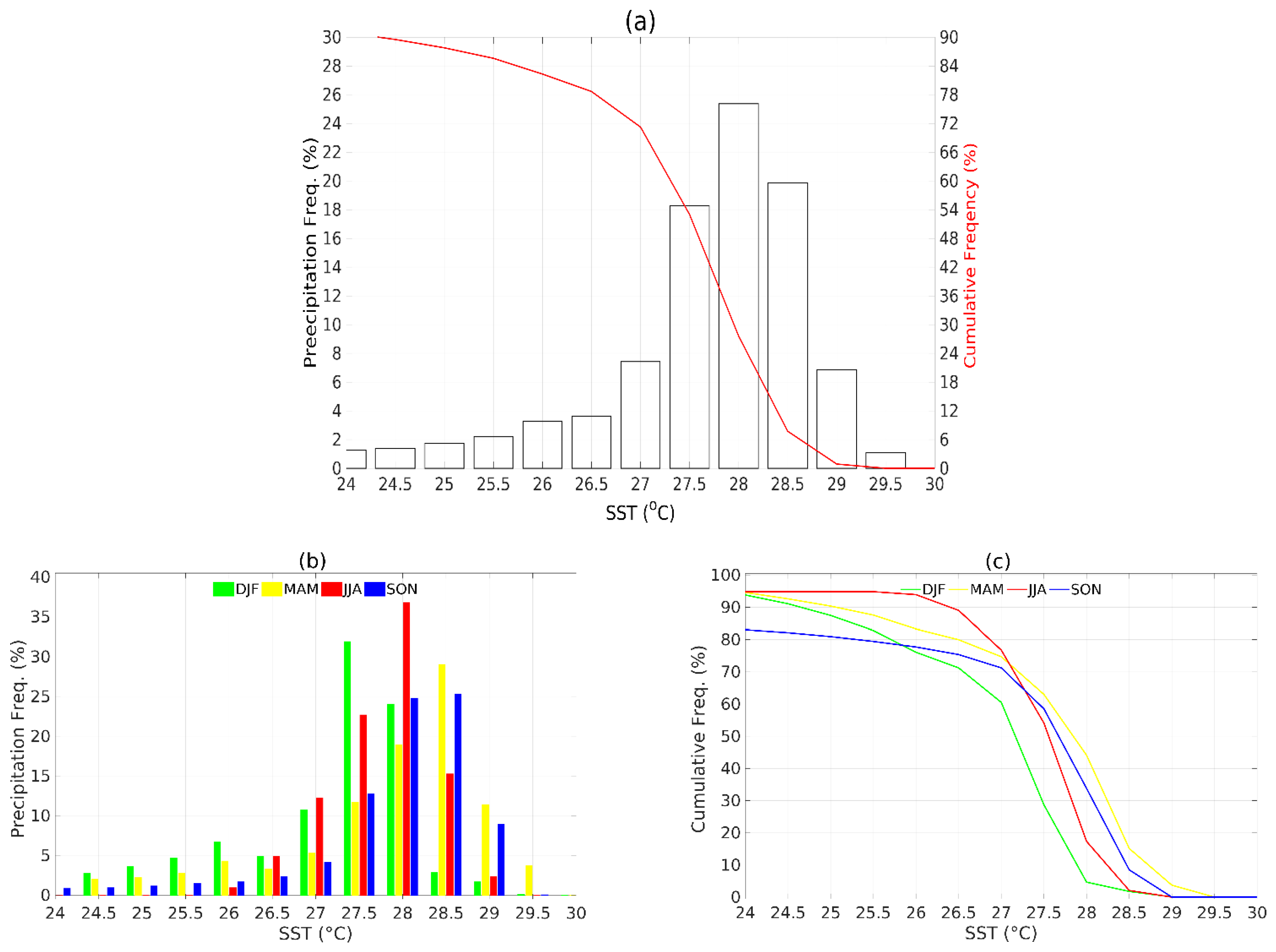
2.2.1. Choice of the Meridional AWP Boundaries

To identify the isotherm associated with the AWP meridional boundaries and with the ITCZ rain band, we quantified the relationship between SST and rainfall. We first calculate the occurrence of rain (greater or equal to 3 mm·d−1) per 0.5 °C range. Figure 2a highlights the non-linearity of the SST-rainfall relationship in the tropical Atlantic, which is characterized by an increase in rainfall distribution that peaks over the 28 °C isotherms. Note the decrease over regions warmer than 28 °C, which is a result that is comparable, albeit for a value of 29 °C, with the one of [14] for the Pacific. This can be explained that there are few regions in the Atlantic with an SST larger than 28°C.
However, the rainfall distribution displays the most significant change for an isotherm of 27 °C, and the cumulative frequency distribution shows that the amount of rainfall increase is lower than 10% for the 0.5 °C steps when one includes further isotherms inferior to 27 °C. On the opposite, as shown by [21], precipitation seems to be very sensitive to variations of high SST. Indeed, we see in Figure 2a that an increase from 27 °C to 27.5 °C corresponds to reinforcement in the frequency by almost 20%. Note, however, that the values depend on longitude. For example, an SST between 27 °C and 27.5 °C is associated with about 16% of the precipitation west of 30° W and about 22% east (not shown). Overall, more than 72% of the precipitation greater than 3 mm·day−1 is noted above the 27 °C isotherm which corresponds to about 79% (67%) east (west) of 30° W respectively (not shown). In this study, the 27 °C isotherm was chosen as a boundary for the AWP, because it is the tipping point in terms of cumulative precipitation.
Figure 2b,c displays the seasonal link between SST and rainfall distribution. Figure 2b shows that the seasonal maxima of the frequency of rainfall distribution are centered on the 27.5 °C isotherm in December-January-February (DJF), 28 °C isotherm in June-July-August (JJA), and 28.5 °C isotherm in March-April-May and September-October-November (MAM and SON). In boreal winter, about 60% of precipitation is observed above 27 °C isotherm. While for the other seasons, more than 70% of the precipitation is located above the AWP. Overall, in the tropical Atlantic, about 70% of precipitation is observed above the 27 °C isotherm.

2.2.2. AWP Migration Velocity Equation

The exact meridional velocities of the Northern and Southern AWP boundaries (corresponding to isotherms 27 °C, hereafter noted NB and SB respectively) is computed as:
V = Δ y Δ t
where Δ y represents the latitude change of an isotherm during ∆t, the time step of the data considered at a given longitude. Since both NB and SB appear during some period at more than one latitude per given longitude (see Figure 1b,c in July for NB and in May for the SB), we retain the latitude closest to the equator. We chose this procedure to follow the strongest ITCZ where significant amounts of precipitation occur. It gives a consequence on the longitudinal averages in the eastern region of 30° W by mixing different regimes. However, this impact is small because a small region of this double WP is considered in the longitudinal average in the eastern region, and processes in this part are weak compared to the average further east during this season (April–July).
In order to distinguish contributions of each oceanic and atmospheric term, we can construct a linear equation of V, using a mixed layer heat budget equation. We first linearize an infinitesimal SST variation in time and latitude (SST is noted T in the following equations).
d T ( y , t ) = T t . d t + T y . d y
In a Lagrangian view, the temperature of a given isotherm verifies:
d T ( y , t ) =   0
Which, using Equation (2), leads to:
d y d t = t T y T
Using Equation (1), we obtain the linearized meridional velocity V* for any isotherm:
V * = t T y T
t T represents the temporal SST changes induced by the ocean and air–sea fluxes into the mixed layer (ML hereafter) and y T the meridional SST gradient.
The heat budget equation of the ML in NEMO [55] quantifies the exact contribution of each process represented by the ocean model to an SST variation, as follows:
t T   =     u . x T v . y T + D l ( T ) Contrib ( 1 )   1 h h t ( T T z = h ) w . z T 1 h ( K z z T ) z = h Contrib ( 2 ) +   Q ns + Q s ( 1 f z = h ) ρ 0 C p h Contrib ( 3 )
where,
o = 1 h h 0 o . d Z
Contrib 1 is the horizontal oceanic processes contribution, Contrib 2 is the vertical oceanic processes contribution, and Contrib 3 represents the air–sea fluxes contribution.
The Mixed Layer (ML) temperature temporal variability is thus due to the sum of each oceanic and atmospheric contribution. In Equation (5), T is the mean temperature in the ML (~=SST), u, v, and w represent the zonal, meridional and vertical components of the current, respectively. Dl(T) is the lateral diffusion, Kz the vertical diffusion coefficient for the tracers, and h the mixed layer depth (MLD). Qns and Qs are the non-solar and solar components of air–sea fluxes respectively, and f(z = −h) the fraction of solar radiation which penetrates into the ML. By replacing t T by its expression (Equation (5)) in Equation (4), we obtain the decomposition of the meridional migration speed of the AWP boundary into a sum of velocities:
V * = V ocean + V air - sea
With,
  V ocean = V oce - lat + V oce - ver V oce - lat = Contrib ( 1 ) y SST , V oce - ver = Contrib ( 2 ) y SST  
V air - sea = V rad - flux + V tur - flux = Contrib ( 3 ) y SST
With V, the velocity of an AWP boundary due to radiative fluxes (shortwave and longwave radiation), while Vtur is that associated with turbulent fluxes (latent and sensible).
One can see that the migration of the AWP boundaries depends on one hand on the values of each contribution, that is in terms of the ML heat budget along the two 27 °C isotherms and on the other hand, is inversely proportional to the local background SST meridional gradient. In other words, for a given SST change, large meridional gradients (as frequently the case in the east) will lead to weaker velocities, hence to a smaller migration, compared to regions with smaller gradients (observed rather to west), that will allow a larger migration. Note also that according to Equation (5) the SST changes, hence the migration velocities, are modulated by the MLD. Hence for a given heat flux into the ML and a given SST gradient, a deeper (shallower) ML causes a slower (faster) migration. In the following, we refer to the meridional SST gradient as y T .

3. Results and Discussion

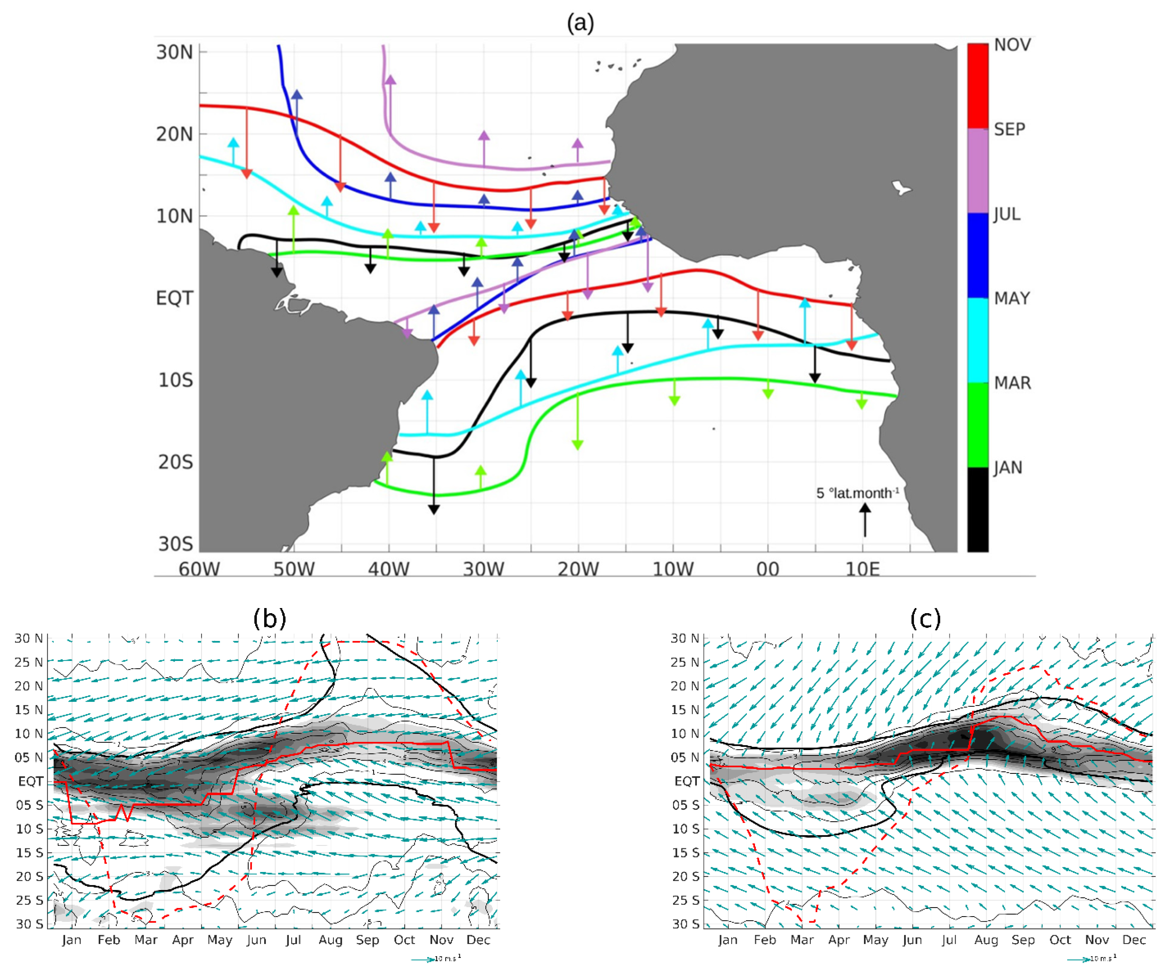
3.1. Description of the ITCZ and AWP Migration

Time–latitude diagrams in Figure 1 indicate that the ITCZ, considered as a Trade winds convergence zone, is essentially comprised between the two 27 °C boundaries and corresponds to the zone of maximum precipitation, as expected from the above diagnostics. However, an analysis by sector shows that this relationship is not always verified; in the W30 (E30) sector the maximum of SST is located south (north) of the convergence and rainfall maxima from January to June (August to October), respectively Figure 1b,c. Note the presence of the double ITCZ centered on 5° S associated with the second maximum of SST and a weak wind convergence, in agreement with previous analyses [4,23].
These characteristics depend, of course, on longitude, and we have divided the basin into two sectors located west and east of 30° W, named W30 and E30 respectively. Indeed, one of the characteristics of the tropical basin is the presence of the Atlantic Cold Tongue (ACT), whose signal in SST is maximum in the E30 sector. This separation also corresponds to the first-order, variations in the distribution of the MLD, thermocline, and wind, and the meridional extension of the AWP and ITCZ, which all shows a strong zonal contrast between the East and the West of the basin.
Most strikingly, the meridional extension of the AWP is wider in the West, reaching as far as 25° S and 25° N, than in the East, limited to 10° S and 15° N (Figure 1). As shown in simplified model experiments [40], this western enlargement is caused by Ekman’s transport towards the poles, and its effect is opposed in the east by the equatorial upwelling cooling. However, it is clear from the orientation difference of wind vectors in Figure 1 that the asymmetry also comes from the more poleward character of this transport in the west, and we will demonstrate this later by measuring the advective contribution to the migration. The role of the eastern upwellings, the equatorial and the two Africans can also be assessed quantitatively as they participate in maintaining strong meridional SST gradients, which have a blocking capacity for meridional AWP movements. Indeed, Equation (4) shows that the V* is inversely proportional to the local y T , that therefore tends to reduce the migration speed. We will quantify this process in detail in Section 3.2.2.
Figure 1 shows that the AWP meridional extension grows in the summer hemisphere and reaches its maximum in the seasonal equinox (March and September). The limit of the AWP in the winter hemisphere is relatively stable. We then focus on the causes associated with the heterogeneity in the migration of the two AWP boundaries in March and September. Figure 1 also shows the existence of a second AWP centered on 5° S in May, more marked in E30, corresponding to the double ITCZ, especially in W30 e.g., [4]. Regarding precipitations, their extensions follow those of the AWP but with some differences in terms of phasing and spatial extension. The southernmost position of precipitation in the south in W30 (along the Brazilian coast) is reached in early May, one month and a half after SB. In terms of extension, the rainfall band in W30 is included in the AWP and is much narrower, while in E30 it coincides more with the AWP, with a greater extension in July–September. Correspondingly, significant rains are observed above the ACT in boreal summer. Note the second band of precipitation south of 20° S, linked to mid-latitudes depressions, is beyond the scope of the paper.
The spatiotemporal correlations between rainfall and SST, quantified in Section 2.2.1, confirm their multifactorial coupling [14,28]. In particular, Figure 1 shows that the convergence zone of the surface winds is generally better associated with the rain band than the AWP, in agreement with the results of [22]. Reference [23] showed the importance of the Laplacian of the SST as the main forcing of the convergence of surface winds, and therefore of rainfall. The homogeneity of the SST in the AWP in W30 near 15° S–10° S corresponds to weak Laplacians associated with weak rainfall amounts (<3 mm·d−1). The same phenomenon is observed for the NB in July–November.
To study the spatiotemporal variability of the AWP described above, we can first take advantage of the Ocean Bucket model [56,57], which is the simplest predictor of SST variations. As a first rough approach, we computed only the solar flux contribution, calculated by taking into account the non-penetrating solar flux in the ML.
The SST solution of this equation is in quadrature-phase (shifted by three months) with respect to the solar flux, and, for the sake of simplicity, only its maximum is shown as a function of time in the time–latitude plots of Figure 1 (red dashed line). For comparison, we have also plotted the maximum of the observed SST (red solid line). Differences between the two curves are due to the effect of the other air–sea fluxes, dominated by the latent heat flux [35] and of the oceanic heat fluxes in the ML. Hence, to the first-order, it appears that this model works well for explaining the phase of the AWP, since both phases are close, and this result underlines the fundamental role of the solar cycle in setting the migration tempo. On the contrary, the migration amplitude is overestimated by far (example: 30°instead of 6°in W30 in March), and this result justifies the detailed analysis of all ML heat flux contributions presented in the rest of the paper. It is also interesting to note the reduction in the migration amplitude of the Bucket SST in E30 from August to November compared to the west. This qualitatively reproduces the zonal contrast underlined above and is most likely due to the blocking effect of strong y T in the east.

3.2. Validation of the Meridional Migration of the AWP Boundaries Simulated by the OGCM and the Linearized Speed Equation

3.2.1. Validation of the AWP Migration Simulated by the OGCM

Several studies have successfully used the NEMO model to study tropical Atlantic SST, in the present configuration [13,33,51] or a comparable one [45]. In the present paper, we focus our work on the meridional velocity V and latitudes of the two AWP meridional boundaries NB and SB. Figure 3 presents time–longitude diagrams of V and latitude, for each meridional boundary, in order to describe them with further details, and compares them with observations. Note that white shading indicates that the 27 °C isotherm is not defined within our domain of study. As observed previously, the highest migration velocities are in the west for NB (Figure 3a) and to a slightly lesser extent for the SB (Figure 3c). The NB migrates poleward from about 6° N up to north of 30° N (out of our model domain), from February to September–October. While the SB migrates poleward from about 28° S in the west and 12° S in the east up to 4° N in the east, from April to August.
Overall, the spatiotemporal variability of the AWP boundary migration speeds simulated by our model is comparable to observations (Figure 3b,d). The errors are higher in the west, where the velocities are the highest. Regarding the NB, errors in latitudes are inferior to two degrees, but velocities are significantly overestimated (more than 10% compared to observations) particularly near July and September to November. SB shows the strongest errors from December to May west of 25° W, and more locally and punctually in the rest of the basin.

3.2.2. Validation of the Linearized Velocity Equation

In order to use the linearized velocity equation (Equation (4)), we now compare V* to the exact velocity V in the OGCM for both boundaries. Figure 4 presents their zonal structure and zonal mean time evolution. For the sake of legibility, only the average from December to February is shown, since it is representative of the entire year or it maximizes the errors. Overall, V and V* are in good agreement in terms of amplitude (Figure 4a,b) and even more in function of time (Figure 4c,d). Note that amplitude errors over the NB west of 35° W (longitude of the tip of the Brazilian coast), are artifacts visible only for such time averages when the isotherm longitudinal extension is rapidly changing along the continental slope.

3.3. Processes Controlling the AWP Meridional Migration Speed

According to Equation (4), V* is controlled by y T the denominator and t T the numerator. Hence the first section of this chapter discusses the respective roles of these two quantities in the spatio-temporal structure of the AWP boundaries meridional velocities. The second chapter provides further analysis of the numerator in the functioning of atmospheric and oceanic heat fluxes effects on the SST, as t T will appear as the key driver of velocity time changes.

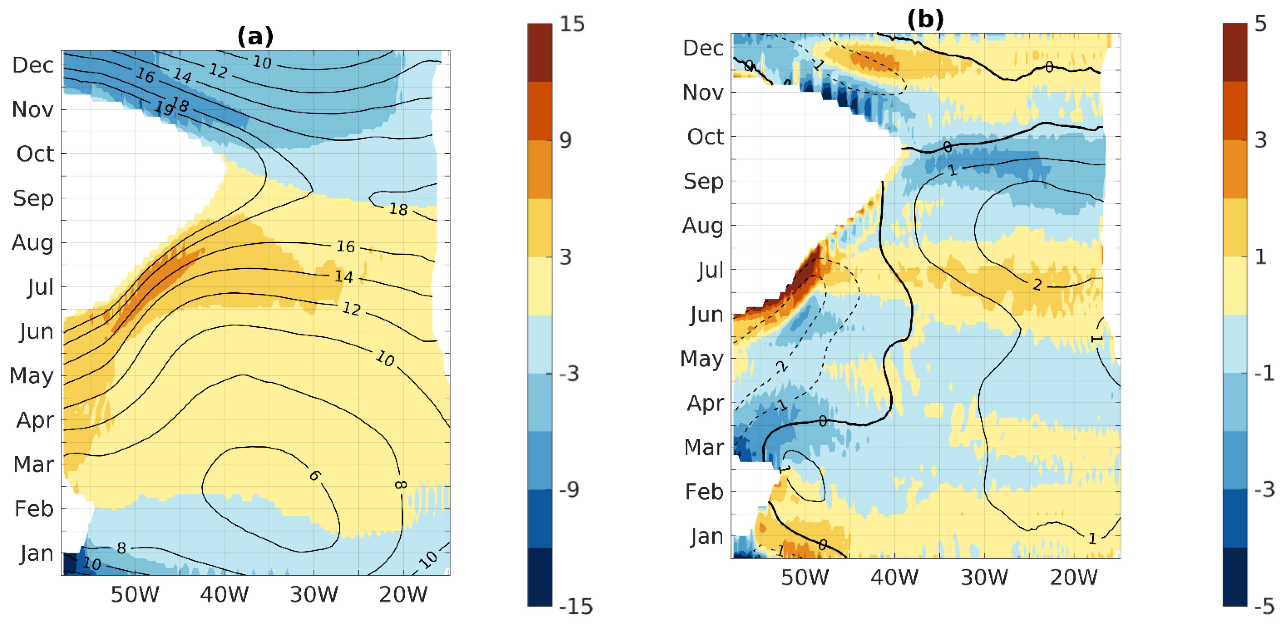
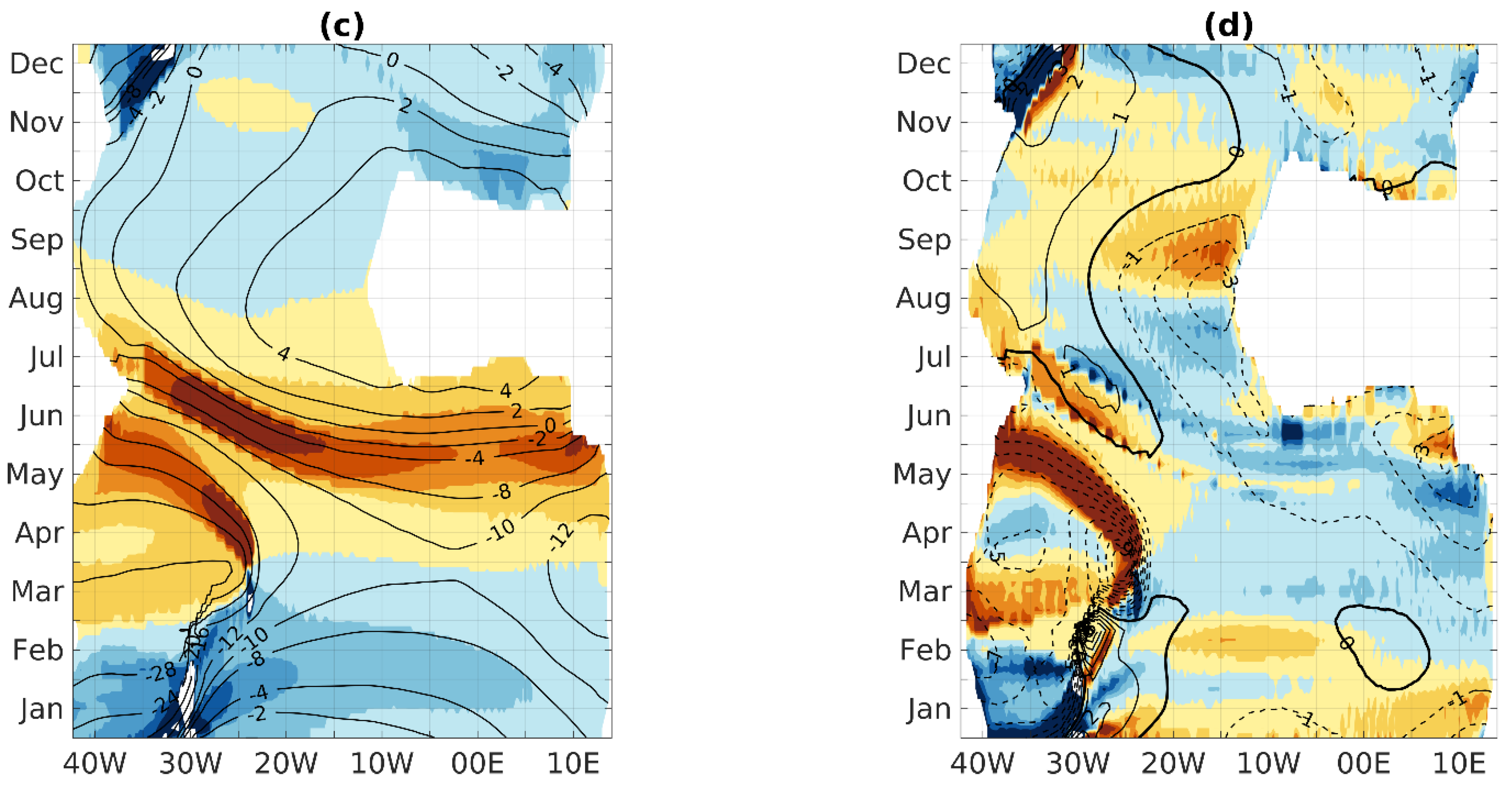
3.3.1. Respective Role of the Meridional SST Gradients and the SST Time-Derivative

The identification of the relative roles of y T and t T in the control of V can be obtained by comparing their relative variations, in function of longitude for the December to February time average (Figure 4a,b), and in function of time in zonal mean over the whole basin (Figure 4c,d). As said before, the results for this season are representative of the entire year. Note that the opposite of y T is displayed for the sake of legibility.
Importantly, since the zonal asymmetry of V is verified by V*, one is allowed to discuss the main causes of this fundamental feature. Regarding NB, Figure 4a demonstrates that the migration velocity decreases eastward due to an overall increase of the norm of y T , generally about twice larger than the changes of t T . This zonal contrast in y T is evidently due to the presence of cold water to the northeast of the NB migration domain, maintained by the Canary upwelling system.
Regarding SB, from a maximum located at 30° W, we note a comparable differential zonal change towards the east of the y T and t T amplitudes (Figure 4b). This can be attributed to the presence of the equatorial upwelling in the center of the basin and the Benguela upwelling system in the east. These results illustrate the strong dependence of the migration amplitudes to the meridional SST gradient.
Regarding the temporal evolution of V, zonal means (Figure 4c,d) show a good agreement between V and V*. Taking into account the fact that the latter mainly follows the variations of t T , in the north as in the south, one can conclude that the SST time derivative, that is the mixed layer temperature changes, controls to the first order the time variations of the migration. In the following, we discuss the causes of such variations in terms of the effects of heat fluxes into the mixed layer.

3.3.2. Role of Heat Fluxes in the Mixed Layer

The aim of this section is to highlight the respective roles of specific ocean and atmosphere ML heat fluxes that add up to the AWP migration velocity V. Since a good estimate of V is offered by V*, we can reason on the basis of the terms of its diagnostic Equation (4), and display in Figure 5 and Figure 6 each contribution, zonally averaged west and east of 30° W. We discuss the balance between oceanic and air–sea fluxes velocities (Equation (6)), followed by more details on their individual constituent according to Equations (7) and (8). First, we note the similarity between V* and Vair-sea (Figure 5a,b and Figure 6a,b) for NB and SB in both longitudinal sectors. Hence, to the first-order, the migration appears dominated by air–sea fluxes, while oceanic heat fluxes act rather as modulators. In the next two sections, we discuss the northern and the southern migration, and since we are interested in highlighting the importance of the ocean specifically, we chose to separate the migration time periods according to the importance and the nature of the oceanic heat fluxes contribution. The slowing effect of vertical mixing in the east explains why the bucket SST model overestimates the migration amplitude there.

Seasonal Migration of the Northern Boundary

During the northward migration, we define a Phase 1 period, like the one corresponding to positive Vocean (see blue line in Figure 5a,b), that is to say, months MAMJ and FMAM for W30 and E30 respectively. Phase 2 follows with a negative Vocean, and ends in late September. During Phase 1, the most striking feature is the prominent role in W30 of the ocean, in setting the starting date of the migration to the end of February, in advance by two months compared to the time (May) when Vair-sea turns poleward. In E30, the same phenomenon occurs only over two weeks, before the air–sea fluxes effect controls entirely the movement, early March. The positive sign of Vocean, which lasts for seven months in W30, can be explained by the analysis of the contributions of horizontal advection (Voce-lat, purple line) and vertical mixing (Voce-ver, purple dash-line) according to Equation (5). Note that in general, in the ML heat budget of the NEMO model in our domain of study, the horizontal ocean processes are significantly dominated by the advection while the vertical terms are dominated by vertical. To the west, the two components of Vocean contribute positively and in-phase (Figure 5c). Voce-lat is associated with poleward advection by Ekman currents [40], forced by zonally oriented intense Trade winds (see Figure 1b), as well as by the Brazil and Guyana Currents close to the continent. Voce-ver corresponds to the effect of vertical mixing with warmer subsurface waters within the vast region of the barrier layer and temperature inversion of the western north-tropical Atlantic [33,58]. On the opposite, the air–sea fluxes contribution slows down the migration, due to latent heat loss cooling exceeding solar warming (Figure 5e) caused by maximum Trade wind speed relative to the east (Figure 1b,c). In the E30 sector (Figure 5d), phase 1 is dominated by a more standard regime, where vertical mixing cools the surface and balances the positive Ekman’s advection, which is relatively weak due to the more meridional orientation of the winds (Vocean close to zero), leading to the control of V by air–sea fluxes effect.
During Phase 2 (June–July to September), V first continues to increase everywhere, through the seasonal intensification of the positive net air–sea fluxes, dominated by the solar heating cycle (Figure 5e,f) and damped by the increasing effect of ocean mixing cooling (Figure 5c,d). Note that the latter is 50% larger in E30 than in W30, due to the incursion of the NB into the Guinea Dome near 12° N and the Canary upwelling open-ocean extension further north, that lifts the thermocline close to the surface [51,59]. Figure 5e,f confirms the earlier interpretation derived from the bucket SST model. The change in the sign of V and the start of the equatorward migration in late September is essentially a direct response to the effect of the solar heat flux cycle in the ML, since the latent heat flux effect is relatively stable at this turning period. Lastly, during boreal winter, the NB continues to respond essentially to the solar forcing but encounters maximum ocean fluxes opposing effects, in early December and late January in E30 and W30 respectively, due to maximum poleward advection, and a temperature inversion warming for the later sector.

Seasonal Migration of the Southern Boundary

For SB, the warming of SST produces evidently southward migration velocities, as expressed in Equation (4) and associated with the positive sign of y T in the southern part of the WP. During the northward migration, the first phase of the negligible ocean fluxes effect is noted from March to mid-June in W30 and from April to mid-May in E30, which is controlled by the cooling effect of the air–sea fluxes (Figure 6a,b). The SB at this time is located far south of the equator, where the SST variability is mainly driven by air–sea fluxes [12,60]. The weak Voce is associated with important values of its two velocity components until the end of April (Figure 6c,d), as the heat advected poleward by southward currents (Voce-lat < 0) is almost entirely transmitted by vertical mixing to the thermocline (Voce-ver − Voce-lat). The migration during this phase appears to be mainly driven by the effect of latent heat loss, larger than that of the solar heat gain (Figure 6e,f).
The second phase is marked by the activation of significant ocean heat fluxes effects, in mid-May in E30 and late June in W30 (Figure 6a,b), when the SB passes 10° South towards the equator. Whereas Vair-sea starts to decrease, the poleward migration speed keeps increasing, as a result of the increase of the SST cooling induced by the equatorial upwelling processes, until June and July, in W30 and E30 respectively. The ocean contribution results from both vertical mixing and horizontal advection (Figure 6c,d), in agreement with earlier studies. To the east where the equatorial SST reaches its minimum, the effect of vertical mixing cooling by the upwelling dominates, whereas to the west, the dominant process is horizontal advection by the northern branch of the SEC of upwelled cold water [41,42]. Regarding the air–sea fluxes effect, it participates to a lesser extent in the poleward movements as it cools the SB (positive Vair-sea) since the southern Trade wind-induced latent heat loss overcomes the declining solar heating. Quantitatively, the upwelling more than doubles V* up to 10°lat.month−1, when Vair-sea peaks at about 4 to 5°lat.mon−1, and the SB is positioned near −9°of latitude. This establishes quantitatively how the equatorial upwelling displaces the southern part of the AWP north of 5° South, up to its northernmost position at about 1° N in July and 5° N in August, west, and east respectively.
Then starts the southward migration until February and March respectively in W30 and E30 (Figure 6a,b). V* follows the air–sea fluxes effect and its amplitude increases during the rest of the period (Figure 6a,b). The increase of the air–sea fluxes effect is explained by solar warming, slightly greater than evaporative cooling at all longitudes. Regarding the ocean role, vertical mixing cooling reduces the migration speed along with the SB during this entire southward migration, to the opposite of surface currents that generally transport the AWP southward, except in November and December near the equator where the NBC and the SEC advect the AWP polewards, especially in the west (Figure 6c,d).

4. Summary and Conclusions

We use observational datasets and an OGCM to study the main mechanisms of the AWP seasonal migration by following its northern and southern boundaries, NB and SB, defined as the 27 °C isotherms. Zonal averages on each side of 30° W, defined as the E30 and W30 sectors, show a good co-localization of the AWP and the ITCZ. Depending on the considered areas and seasons, 60% to 80% of the rainfall greater than 3 mm·day−1 is shown in the region where the temperature exceeds 27 °C.
We have shown that the meridional migration speed V, for NB as well as SB, can be realistically expressed, to the first-order, as V* the ratio between the SST time derivative and the meridional SST gradient across a chosen isotherm (Equation (4)). Firstly, it allows us to demonstrate that the striking longitudinal contrast in the AWP behavior (i.e., migration amplitude growing from about 10 degrees of latitude along Africa to up to 20 degrees along the Americas) is mainly explained by the strong meridional SST gradients to the east. They are associated with the equatorial and eastern boundary upwelling systems and weaken migration there. Secondly, V* was formulated as the sum of migration velocities, each associated with one of the terms of the equation of the mixed layer temperature time evolution. This breakdown led to the identification of different migration regimes as a function of time, for given longitudes and each boundary, according to the processes dominating the mixed layer heat budget. Figure 7 and Figure 8 summarize our results by presenting these regimes, for the northward and southward migration phases respectively. For the largest part of the year, V is controlled by the effect of the net air–sea heat flux, while oceanic processes only modulate its amplitude. However, we identified two major exceptions. One in the west in MAM for the NB, and the other in JJA for the SB at all longitudes. The sign and the intensity of this modulation by oceanic processes were used as criteria to differentiate between two sub-periods of the northward and southward phases of migration.
The AWP northward migration begins roughly in March. During the first phase, characterized by a positive or negligible oceanic contribution, the AWP migrates as a whole with increasing speed, approximately until May–June. In the northwest, the solar radiation effect, which increases in time, remains lower than that of the latent heat loss by maximum Trade winds, resulting in a net air–sea forcing of the NB to migrate equatorward. Its actual northward displacement is due to warming by oceanic processes, consisting of northward advection by Ekman transport, the South Equatorial Current (SEC), and the Guyana Current (GuyC), as well vertical mixing warming within the vast temperature inversion zone of the northwest tropical Atlantic (Figure 7, first and second poleward arrows). To the northeast of the NB and southeast of the SB, the poleward advection effect of the Ekman currents and the South Brazilian Current (SBC) along the west coast is canceled by vertical mixing with the cold waters of the thermocline (Figure 7, upper right and lower left, two first arrows). Migration is thus essentially controlled by air–sea fluxes, which warm (cool) to the north (south). The warming to the northeast is explained by the solar radiation effect being greater than that of evaporation in the minimum zone of the Trade wind. Whereas the cooling to the south is explained by the seasonal decrease in solar radiation and increase in latent heat loss, as the Trade winds approach their maximum.
The second phase of northward migration takes place from June to August (until September in the northwest) and is characterized by an amplification of cooling by oceanic processes. This later significantly amplifies the role of the ocean relative to that of the atmosphere, except in the northwest where it makes it negligible. For the NB, displacement accelerates and mainly responds to the increasing effect of the solar flux. In the northwest, the NB passes north of the barrier layer region, where vertical mixing moderately cools the surface (deep thermocline region) and advection is weak. In the northeast, strong oceanic cooling slows migration and is due to intensified vertical mixing in the Guinea dome and the West African coastal upwelling region. In the south, the SB crosses the equator during the intensification of the equatorial upwelling. The intensely cooling oceanic processes associated with the cold tongue have an effect greater than that of the decreasing air–sea fluxes. In the west, the northern branch of the SEC brings the SB to the north, while in the center and east, vertical mixing of the upwelling dominates. We could quantify the dominant role of the upwelling in moving the AWP north of 5° South in July and August, west and east respectively.
Southward migration starts in September to the north and south. For NB, there is a certain homogeneity in the mechanisms, dominated by the effects of air–sea fluxes via evaporative cooling. This displacement is significantly mitigated by oceanic processes that induce warming from November onwards in both sectors (Figure 8, grey isotherm). Subsequently, in the west, NB returns to the temperature inversion region where the ocean induces strong warming via vertical mixing and Ekman transport. In the east, the cooling effect of the vertical mixing in the Guinea Dome region diminishes rapidly as winter approaches in favor of poleward Ekman transport which mitigates the migration. For SB, the southward migration is explained by the effects of air–sea fluxes via solar heating (greater than evaporative cooling), mitigated by the strengthening of cooling by vertical mixing. In the East, SB passes again in the equatorial upwelling region where the strong vertical mixing cooling slows down the migration.
Overall, our results indicate that the ocean is often a brake on the migration imposed by the net air–sea flux. However, it is a driving force in the boreal spring in the northwest, where it removes the heat accumulated under the barrier layers zone, and in the boreal spring and summer near the equator where the equatorial upwelling drives the AWP northward. The use of our diagnostic equation for isotherm velocities can be generalized to the quantification of the causes of anomalies in the positioning of the AWP and ITCZ relative to the seasonal cycle, at intra-seasonal and lower frequencies.
The dominant effect of air–sea fluxes demonstrated here indicates that it is essential, in tropical climate modeling, to continue to improve the observation and simulation of heat exchanges at the ocean–atmosphere interface. Climate models, which are marked by significant errors in the meridional position of the ITCZ and associated coastal precipitation [59,61], also need a better representation of the mixed layers of the atmosphere and ocean, and thus the heat exchange between the two environments. The importance of the SST mixed layer temperature and meridional SST gradients for the modulation of the WP migration rates argues for the continuing improvement of realism in ocean and climate models.

Author Contributions

Conceptualization: D.W., A.L., M.W. and A.T.G. Methodology: D.W., M.W. and A.L. Software: D.W. and M.W. Validation: D.W., A.L., M.W. Formal analysis: D.W., A.L. and M.W. Investigation: D.W., A.L., M.W. and A.T.G. Resources: A.T.G. and A.L. Data curation: D.W. Writing—original draft preparation: D.W., A.L., M.W. and A.T.G. Writing—review and editing: D.W. A.L. and M.W. Visualization: D.W., A.L. and M.W. Supervision: A.T.G. and A.L. Project administration: A.T.G. and A.L. Funding acquisition: A.T.G. and A.L. All authors have read and agreed to the published version of the manuscript.” Please turn to the CRediT taxonomy for the term explanation. Authorship must be limited to those who have contributed substantially to the work reported.

Funding

CEAMITIC.

Institutional Review Board Statement

Not applicable.

Informed Consent Statement

Not applicable.

Data Availability Statement

Data are freely available.

Acknowledgments

The authors thank the Laboratoire de Physique de l’Atmosphère et de l’Océan Siméon Fongang (LPAO-SF) of the University Cheikh Anta Diop de Dakar where the work was mainly done. The editor and the anonymous reviewers are also sincerely thanked for their valuable comments and suggestions to improve the quality of the paper. The research leading to these results has received funding from the Centre d’Excellence Africain en Mathématiques, Informatique et Technologie de l’Information et de la Communication (CEA-MITIC). We also thank the Laboratoire Mixte International (LMI ECLAIRS) and Science for weather information and forecasting techniques (SWIFT) project for their essential financial support during this study. We thank Anne-Charlotte Peter for her essential contribution in setting up the ATLTROP025 configuration and running the simulation.

Conflicts of Interest

The authors declare no conflict of interest.

References

  1. Ninomiya, K. Similarity and Difference between the South Atlantic Convergence Zone and the Baiu Frontal Zone Simulated by an AGCM. J. Meteo. Soc. Jpn. 2007, 85, 277–299. [Google Scholar] [CrossRef] [Green Version]
  2. Villela, R.J. The south atlantic convergence zone: A critical view and overview. Rev. Do Inst. Geológico São Paulo 2017, 38, 1–19. [Google Scholar] [CrossRef] [Green Version]
  3. Schneider, T.; Bischoff, T.; Haug, G.H. Migrations and dynamics of the inertropical convergence zone. Nature 2014, 513. [Google Scholar] [CrossRef] [PubMed]
  4. Liu, W.T.; Xie, X. Double intertropical convergence zones—A new look using scatterometer. Geophys. Res. Lett. 2002, 29, 2072. [Google Scholar] [CrossRef] [Green Version]
  5. Tomaziello, A.C.N.; Carvalho, L.M.V.; Gandu, A.W. Intraseasonal variability of the Atlantic Intertropical Convergence Zone during austral summer and winter. Clim. Dyn. 2016. [Google Scholar] [CrossRef]
  6. Yu, L.; Jin, X.; Weller, R.A. Role of Net Surface Heat Flux in Seasonal Variations of Sea Surface Temperature in the Tro Atlantic Ocean. J. Clim. 2006, 19, 6153–6169. [Google Scholar] [CrossRef]
  7. Fasullo, J.; Webster, P.J. Warm Pool SST Variability in Relation to the Surface Energy Balance. J. Clim. 1998, 12, 1292–1305. [Google Scholar] [CrossRef]
  8. Rajendran, K.; Gadgil, S.; Surendran, S. Monsoon season local control on precipitation over warm tropical oceans. Meterol. Atmos. Phys. 2019, 131, 1451–1465. [Google Scholar] [CrossRef]
  9. Graham, N.E.; Barnett, T.P. Sea surface Temperature, Surface Wind Divergence, and Convection over Tropical Oceans. Report 30 October 1987. Available online: http://www.sciencemag.org/ (accessed on 28 November 2014).
  10. He, J.; Johnson, N.C.; Vecchi, G.A.; Kirtman, B.; Wittenberg, A.T.; Sturm, S. Precipitation Sensitivity to Local Variations in Tropical Sea Surface Temperature. J. Clim. 2018, 31, 9225–9238. [Google Scholar] [CrossRef] [Green Version]
  11. Oueslati, B.; Bellon, G. The double ITCZ bias in CMIP5 models: Interaction between SST, large-scale circulation and precipitation. Clim Dyn. 2015, 44, 585–607. [Google Scholar] [CrossRef]
  12. Waliser, D.E.; Graham, N.E. Convective Cloud Systems and Warm-Pool Sea Surface Temperatures: Coupled Interactions and Self-Regulation. J. Geophys. Res. 1993, 98, 12881–12893. [Google Scholar] [CrossRef]
  13. Okumura, Y.; Xie, S.P. Interaction of the Atlantic Equatorial Cold Tongue and the African Monsoon. J. Clim. 2004, 17, 3589–3602. [Google Scholar] [CrossRef] [Green Version]
  14. Lin, B.; Wielicki, B.A.; Minnis, P.; Lin, C.; Xu, K.M.; Hu, Y. The effect of Environmental Conditions on Tropical Deep Convective Systems Observed from the TRMM Satellite. J. Clim. 2006, 19, 5745–5761. [Google Scholar] [CrossRef] [Green Version]
  15. Xie, S.P.; Carton, J.A. Tropical Atlantic Variability: Patterns, Mechanisms, and Impacts. In Geophysical Monograph; AGU: Washington, DC, USA, 2004. [Google Scholar]
  16. Cintra, M.M.; Lentini, C.A.D.; Servain, J.; Araujo, M.; Marone, E. Physical processes that drive the seasonal evolution of the Southwestern Tropical Atlantic Warm Pool. Dyn. Atmos. 2015, 72, 1–11. [Google Scholar] [CrossRef]
  17. Kim, S.T.; Yu, J.-Y.; Lu, M.-M. The distinct behaviors of Pacific and Indian Ocean warm pool properties on seasonal and interannual time scales. J. Geophys. Res. 2012, 117, D05128. [Google Scholar] [CrossRef] [Green Version]
  18. Shi, W.; Xiao, Z.; AI, Y. The behavior of deep convective clouds over the warm pool and connection to the Walker circulation. Sci. China Earth Sci. 2018, 61, 1605–1621. [Google Scholar] [CrossRef]
  19. Wang, C.; Enfield, D.B. The tropical Western Hemisphere warm pool. Geophys. Res. Lett. 2001, 28, 1635–1638. [Google Scholar] [CrossRef]
  20. Gill, A.E. Some simple solutions for heat-induced tropical circulation. Quart. J. Met. Soc. 1980, 106, 447–462. [Google Scholar] [CrossRef]
  21. Biasutti, M.; Battisti, D.S.; Sarachick, E.S. Mechanisms Controlling the Annual Cycle of Precipitation in the Tropical Atlantic Sector in an Atmospheric GCM. J. Clim. 2004, 17, 4708–4723. [Google Scholar] [CrossRef] [Green Version]
  22. Back, L.E.; Bretherthon, C.S. On the Relationship between SST Gradients, Boundary Layer Winds, and Convergence over Tropical Oceans. J. Clim. 2009, 22, 4182–4196. [Google Scholar] [CrossRef]
  23. Diakhaté, M.; Lazar, A.; de Coëtlogon, G.; Gaye, A.T. Do SST gradients drive the monthly climatological surface wind convergence over the tropical Atlantic? Int. J. Climatol. 2018. [Google Scholar] [CrossRef]
  24. Stevens, B.; Duan, J.J.; Mc Williams, J.C.; Münnich, M.; Neelin, D. Entrainment, Rayleigh friction, and boundary layer winds over tropical Pacific. J. Clim. 2002, 648, 30–44. [Google Scholar] [CrossRef]
  25. Waliser, D.E.; Jiang, X. Intertropical Convergence Zone. Atmos. Sci. 2015, 6, 121–131. [Google Scholar] [CrossRef]
  26. Giannini, A.; Saravanan, R.; Chang, P. Dynamics of the boreal summer African monsoon in the NSIPP1 atmospheric model. Clim. Dyn. 2005, 25, 517–535. [Google Scholar] [CrossRef]
  27. Sultan, B.; Janicot, S. Abrupt shift of the ITCZ over West Africa and intra-seasonal variability. Geophys. Res. Lett. 2000, 27, 3353–3356. [Google Scholar] [CrossRef]
  28. Sultan, B.; Janicot, S. The West African Monsoon Dynamics. Part II: The « Preonset » and « Onset » of the Summer Monsoon. J. Clim. 2003, 16, 3407–3427. [Google Scholar] [CrossRef]
  29. Hastenrath, S. Circulation and teleconnection mechanisms of Northeast Brazil droughts. Prog. Oceanogr. 2006, 407–415. [Google Scholar] [CrossRef]
  30. Hounsou-gbo, G.A.; Araujo, M.; Bourlès, B.; Veleda, D.; Servain, J. Tropical Atlantic Contributions to Strong Rainfall Variability Along the Northeast Brazilian Coast. Adv. Meteorol. 2015. [Google Scholar] [CrossRef] [Green Version]
  31. Nobre, P.; Shukla, J. Variations of Sea Surface Temperature, Wind Stress, and Rainfall over the Tropical Atlantic and South America. J. Clim. 1996, 9, 2464–2479. [Google Scholar] [CrossRef]
  32. Donders, T.H.; de Boer, H.J.; Finsinger, W.; Grimm, E.C.; Dekker, S.C.; Reichart, G.J.; Wagner-Cremer, F. Impact of the Atlantic Warm Pool on precipitation and temperature in Florida during North Atlantic cold spells. Clim. Dyn. 2011, 36, 109–118. [Google Scholar] [CrossRef] [Green Version]
  33. Liu, H.; Wang, C.; Lee, S.K.; Enfield, D. Inhomogeneous influence of the Atlantic warm pool on United States precipitation. Atmos. Sci. Let. 2015, 16, 63–69. [Google Scholar] [CrossRef]
  34. Misra, V.; Groenen, D.; Bhardwaj, A.; Mishra, A. The warm pool variability of the tropical northeast Pacific. Int. J. Climatol. 2016, 36, 4625–4637. [Google Scholar] [CrossRef]
  35. Wang, C.; Zhang, L.; Lee, S.K. Response of Freshwater Flux and Sea Surface Salinity to Variability of the Atlantic Warm Pool. J. Clim. 2013, 26, 1249–1267. [Google Scholar] [CrossRef]
  36. Wang, C.; Enfield, D.B.; Lee, S.K.; Landsea, C.W. Influences of the Atlantic Warm Pool on Western Hemisphere Summer Rainfall and Atlantic Hurricanes. J. Clim. 2006, 19, 3011–3028. [Google Scholar] [CrossRef]
  37. Philander, S.G.H.; Gu, D.; Halpern, D.; Lambert, G.; Lau, N.C.; Li, T.; Pacanowski, R.C. Why the ITCZ Is Mostly North of the Equator. J. Clim. 1996, 9, 2958–2972. [Google Scholar] [CrossRef] [Green Version]
  38. Frierson, D.M.W.; Hwang, Y.T. Extratropical Influence on ITCZ Shifts in Slab Ocean Simulations of Global Warming. J. Clim. 2012, 25, 720–733. [Google Scholar] [CrossRef] [Green Version]
  39. Kang, S.; Frierson, D.M.; Held, I.M. The Tropical Response to Extratropical Thermal Forcing in an Idealized GCM: The Importance of Radiative Feedbacks and Convective Parameterization. J. Atmos. Sci. 2009. [Google Scholar] [CrossRef] [Green Version]
  40. Clement, A.C.; Seager, R.; Murtugudde, R. Why Are There Tropical Warm Pools? J. Clim. 2005, 18, 5294–5311. [Google Scholar] [CrossRef]
  41. Jouanno, J.; Marin, F.; Penhoat, Y.; Sheinbaum, J.; Molines, J.M. Seasonal heat balance in the upper 100 m of the equatorial Atlantic Ocean. J. Ceophys. Res. 2011, 116, C09003. [Google Scholar] [CrossRef] [Green Version]
  42. Peter, A.C.; Le Hénaff, M.; du Penhoat, Y.; Menkes, C.E.; Marin, F.; Vialard, J.; Caniaux, G.; Lazar, A. A model study of the seasonal mixed layer heat budget in the equatorial Atlantic. J. Geophys. Res. 2006, 111, C0014. [Google Scholar] [CrossRef] [Green Version]
  43. Misra, V.; Stroman, A.; DiNapoli, S. The rendition of the Atlantic Warm Pool in the reanalyses. Clim. Dyn. 2013, 41, 517–532. [Google Scholar] [CrossRef]
  44. Wade, M.; Caniaux, G.; du Penhoat, Y.; Dengler, M.; Giordani, H.; Hummels, R. A one-dimensional modeling study of the diurnal cycle in the equatorial Atlantic at the PIRATA buoys during the EGEEE-3 campaign. Oce. Dyn. 2010, 61, 1–20. [Google Scholar] [CrossRef]
  45. Huffman, G.J.; Bolvin, D.T. Version 1.2 GPCP One-Degree Daily Precipitation Data Set Documentation. NASA Goddard Space Flight Cent. Rep. 2013, 27. Available online: hftp://meso.gsfc.nasa.gov/pub/1dd-v1.2/1DD_v1.2_doc.pdf (accessed on 28 November 2014).
  46. Reynolds, R.W.; Smith, T.M.; Liu, C.; Chelton, D.B.; Casey, K.S.; Schlax, M.G. Daily High-Resolution-Blended Analyses for Sea Surface Temperature. J. Clim. 2007, 20, 5473–5496. [Google Scholar] [CrossRef]
  47. Praveen Kumar, B.; Vialard, J.; Lengaigne, M.; Murty, V.S.N.; McPhaden, M.J. TropFlux: Air-sea fluxes for the global tropical oceans-description and evaluation. Clim. Dyn. 2012, 38, 1521–1543. [Google Scholar] [CrossRef]
  48. Brodeau, L.; Barnier, B.; Tréguier, A.; Penduff, T.; Gulev, S. An ERA40-based atmospheric forcing for global ocean circulations models. Ocean. Model. 2010, 31, 88–104. [Google Scholar] [CrossRef] [Green Version]
  49. Madec, G. NEMO Ocean Engine. In Note Pôle Modèle; Inst. Pierre-Simon Laplace: Paris, France, 2008; Volume 77. [Google Scholar]
  50. Roullet, G.; Madec, G. Salt conservation, free surface, and varying levels: A new formulation for ocean general circulation models. J. Geophys. Res. 2000, 105, 23927–23942. [Google Scholar] [CrossRef]
  51. Faye, S.; Lazar, A.; Sow, B.A.; Gaye, A.T. A model study of the seasonality of sea surface temperature and circulation in the Atlantic North-eastern Tropical Upwelling System. Front. Phys. 2015, 3, 76. [Google Scholar] [CrossRef] [Green Version]
  52. Molines, J.M.; Barnier, B.; Penduff, T.; Brodeau, L.; Treguier, A.M.; Theetten, S.; Madec, G. Definition of the Interannual Experiment Orca025-g70, 1958 2004. Technical Report; Laboratire des Ecoulements Geophysiques et Industriels, CNRS UMR 5519: Grenoble, France, 2007. [Google Scholar]
  53. Large, W.G.; Yeager, S.G. Diurnal to Decadal Global Forcing For Ocean and Sea-Ice Models: The Data Sets and Flux Climatologies. Natl. Cent. Atmos. Res. 2004, 11, 324–336. [Google Scholar]
  54. Zhang, Y.; Rossow, W.B.; Lacis, A.A.; Oinas, V.; Mishchenko, M.I. Calculation of radiative fluxes from the surface to top of atmosphere based on ISCCP and other global data sets: Refinements of the radiative transfer model and the input data. J. Geophys. Res. 2004, 109, D19105. [Google Scholar] [CrossRef] [Green Version]
  55. Vialard, J.; Menkes, C.; Boulanger, J.P.; Delecluse, P.; Guilyardi, M.; McPhaden, M.J.; Madec, G. A Model Study of Oceanic Mechanisms Affecting Equatorial Pacific Sea Surface Temperature during the 1997-98 El Nino. J. Phys. Oce. 2001, 31, 1649–1675. [Google Scholar] [CrossRef] [Green Version]
  56. Carella, G.; Morris, A.K.R.; Pascal, R.W.; Yelland, M.J.; Berry, D.I.; Morak-Bozzo, S.; Merchant, C.J.; Kent, E.C. Measurements and models of the temperature change of water samples in sea-surface temperature buckets. Q. J. R. Meteorol. Soc. 2017, 143, 2198–2209. [Google Scholar] [CrossRef] [Green Version]
  57. Cayan, D.R. Latent and Sensible Heat Flux Anomalies over the Northern Oceans: Driving the Sea Surface Temperature. J. Phys. Oceanogr. 1992, 22, 859–881. [Google Scholar] [CrossRef]
  58. De Boyer Montégut, C.; Vialard, J.; Shenoi, S.S.; Shankar, D.; Durand, F.; Ethé, C.; Madec, G. Simulated Seasonal and Interannual Variability of the Mixed Layer Heat Budget in the Northern Indian Ocean. J. Clim. 2007, 20, 3249–3268. [Google Scholar] [CrossRef]
  59. Doi, T.; Vecchi, G.A.; Rosati, A.J.; Delworth, T.L. Biases in the Atlantic ITCZ in Seasonal-Interannual Variations for a Coarse and a High-Resolution Coupled Climate Model. J. Clim. 2012, 25, 5494–5511. [Google Scholar] [CrossRef]
  60. Carton, J.A.; Cao, X.; Giese, B.S.; da Silva, A.M. Decadal and interannual SST variability in the tropical Atlantic Ocean. J. Phys. Oceanogr. 1996, 26, 1165–1175. [Google Scholar] [CrossRef] [Green Version]
  61. Richter, I.; Xie, S.P.; Morioka, Y.; Doi, T.; Taguchi, B.; Behera, S. Phase locking of equatorial Atlantic variability through the seasonal migration of the ITCZ. Clim. Dyn. 2016, 48, 3615–3629. [Google Scholar] [CrossRef]
Figure 1. Spatio-temporal climatological variations of the Atlantic Warm Pool derived from observations. (a) Northern and southern 27 °C boundary isotherms (color lines) and migration meridional velocity (° lat.month−1, vectors), monthly averaged, spatially low-pass filtered, plotted every other month. (b,c) Time-latitude diagrams of surface wind convergence (s−1, color), rain (mm·day−1, black contour), 10 m wind (m.s−1, vectors), 27 °C isotherms (bold black line), maximum SST (red line), and maximum SST for the bucket model (red dashed line). Zonal average over the 60° W–30° W (b) and the 30° W–15° E (c) sectors.
Atmosphere 12 01224 g001
Figure 2. (a) Diagrams of rainfall distribution frequency (mm·day−1) by 0.5 °C SST band: on the tropical Atlantic (60° W–15° E; 30° S–30° N), cumulative frequency (%, red line). (b,c) Diagrams of the distribution frequency and cumulative frequency (%), respectively, by season. Here, only maritime precipitations greater or equal to 3 mm·day−1 are considered.
Atmosphere 12 01224 g002
Figure 3. Migration velocities (°lat/month, color) and meridional position (°lat, contour) of NB (a) and SB (c). Absolute bias, compared to observational datasets SST Reynolds, in migration speed (°lat/month, color) and meridional position (°lat, contour) for NB (b) and SB (d). Regarding the bias, negative (positive) values of position bias are shown in continuous (dashed) contours. For a better representation, we have chosen not to show latitudes above 19° N for the NB.
Atmosphere 12 01224 g003aAtmosphere 12 01224 g003b
Figure 4. Comparison of V and V* and dependance on dyT and dtT along NB and SB. Zonal structure in time average from December to February (DJF, a,b) and time evolution in zonal average (c,d), exact AWP boundaries migration speed V (°lat/month, blue), linearized AWP boundaries migration speed V* (°lat/month, cyan), meridional SST gradient multiplied by (−1) (°C/°lat, black), and SST time-derivative (°C/month, red). Along the NB (a,c) and the SB (b,d).
Atmosphere 12 01224 g004
Figure 5. Velocity contributions (°lat.month−1) for NB, averaged over the W30 (left) and E30 (right) sectors. (a,b) Total velocity (V*, black), contributions of air–sea fluxes (Vair-sea, red) and oceanic processes (Vocean, blue), and NB latitude (magenta). (c,d) Contributions of lateral oceanic processes (Voce-lat, light blue) and vertical oceanic processes (Voce-ver, dashed light blue). (e,f) Contributions of radiative (Vrad-flux, light red) and turbulent (Vtur-flux, dashed light red) fluxes. Grey shading indicates the northward migration period.
Atmosphere 12 01224 g005
Figure 6. Same as Figure 5, but for the AWP southern boundary (SB). For a better comparison, the Vrad-flux is multiplying by (−1).
Atmosphere 12 01224 g006
Figure 7. Schematic representation of the AWP northward migration mechanism during boreal Spring (April, grey contour) and Summer (July, cyan contour). Meridional linear velocities (vectors) grouped by three which add up to V*, Voce-ver (left arrow), Vocea-lat (middle arrow), and Vair-sea fluxes (right arrow). Northward (southward) arrows represent positive (negative) velocities and their color reminds the sign of the heat flux: warming (red) and cooling (blue). The amplitude of the meridional SST gradient is represented by the gradient symbol. BL: barrier layer, GD: Guinea Dome, SEC: South Equatorial Current, Ek: Ekman transport, GuyC: Guyana Current, NBC: North Brazil Current, and SBC: Southern Brazil Current. Cup: Canary Upwelling System, EqUp: Equatorial Upwelling, and BUp: Benguela Upwelling system.
Atmosphere 12 01224 g007
Figure 8. Same as Figure 7, but for the AWP southward migration during boreal autumn (November, grey contour) and boreal winter (January, cyan contour).
Atmosphere 12 01224 g008
Publisher’s Note: MDPI stays neutral with regard to jurisdictional claims in published maps and institutional affiliations.

