Technical Note

Evaluation of Using Satellite-Derived Aerosol Optical Depth in Land Use Regression Models for Fine Particulate Matter and Its Elemental Composition

1
Institute of Environmental and Occupational Health Sciences, National Taiwan University, Room 717, No.17, Xu-Zhou Road, Taipei 100, Taiwan
2
Center for Space and Remote Sensing Research, National Central University, Taoyuan 320, Taiwan
3
Department of Environmental Engineering, National Cheng Kung University, Tainan 701, Taiwan
4
Department of Public Health, National Taiwan University, Taipei 100, Taiwan
*
Author to whom correspondence should be addressed.
Atmosphere 2021, 12(8), 1018; https://doi.org/10.3390/atmos12081018
Submission received: 2 July 2021 / Revised: 23 July 2021 / Accepted: 5 August 2021 / Published: 8 August 2021

Abstract

:
This study introduced satellite-derived aerosol optical depth (AOD) in land use regression (LUR) modeling to predict ambient concentrations of fine particulate matter (PM2.5) and its elemental composition. Twenty-four daily samples were collected from 17 air quality monitoring sites (N = 408) in Taiwan in 2014. A total of 12 annual LUR models were developed for PM2.5 and 11 elements, including aluminum, calcium, chromium, iron, potassium, manganese, sulfur, silicon, titanium, vanadium, and zinc. After applied AOD and a derived-predictor, AOD percentage, in modeling, the number of models with leave-one-out cross-validation R2 > 0.40 significantly increased from 5 to 9, indicating the substantial benefits for the construction of spatial prediction models. Sensitivity analyses of using data stratified by PM2.5 concentrations revealed that the model performances were further improved in the high pollution season.

1. Introduction

Many epidemiological studies have revealed that exposure to particulate matter with an aerodynamic diameter less than 2.5 µm (PM2.5) is associated with adverse health effects [1,2,3,4]. In recent years, an increasing number of studies focused on source-specific PM2.5 and associated composition because they may affect human health more specifically [5,6,7,8,9]. For example, wood combustion, which is mainly characterized by potassium (K), was found having a strong association with mortality [8].
To predict the exposure to air pollutants, land use regression (LUR) models were developed based on air pollutants acquired at numerous locations and surrounding land use information extracted using geographic information system (GIS) as predictor variables [10,11]. On the basis of variables selected in the final models, critical sources of air pollutants can be identified [12,13,14,15].
The LUR model has been employed to predict the spatial distribution of PM2.5-bound elemental composition in previous studies [16,17,18,19,20,21,22,23]. However, most of these studies were conducted in the United States, Europe, and Australia. Because culture-specific sources (e.g., burning of joss sticks and papers in Chinese temples) may contribute to PM2.5 composition, developing the LUR model to study PM2.5 composition sources in Asia is crucial. Hsu et al. [17] developed LUR models using the satellite-derived data of vegetation index for PM2.5 composition based on repeated measurements at six monitoring sites in Taiwan. The composition with good model performance (R2 ≥ 0.50) include ammonium (NH4+), sulfate (SO42-), nitrate (NO3-), organic carbon (OC), elemental carbon (EC), barium (Ba), manganese (Mn), copper (Cu), zinc (Zn), and antimony (Sb). Nevertheless, the limited number of monitoring sites might restrict its applicability to predict the spatial variation of PM2.5 composition in a wide area. Furthermore, the utility of other satellite data (e.g., aerosol optical depth, AOD) was not explored in Hsu et al.’s study. In general, land use information indicates the surface emission solely while the satellite AOD includes the transport part of pollutants.
In this technical note, LUR models were constructed for PM2.5, aluminum (Al), calcium (Ca), chromium (Cr), iron (Fe), potassium (K), Mn, sulfur (S), silicon (Si), titanium (Ti), vanadium (V), and Zn composition based on 17 monitoring sites in Taiwan. The efficacy of utilizing satellite-derived AOD was also evaluated.

2. Material and Methods

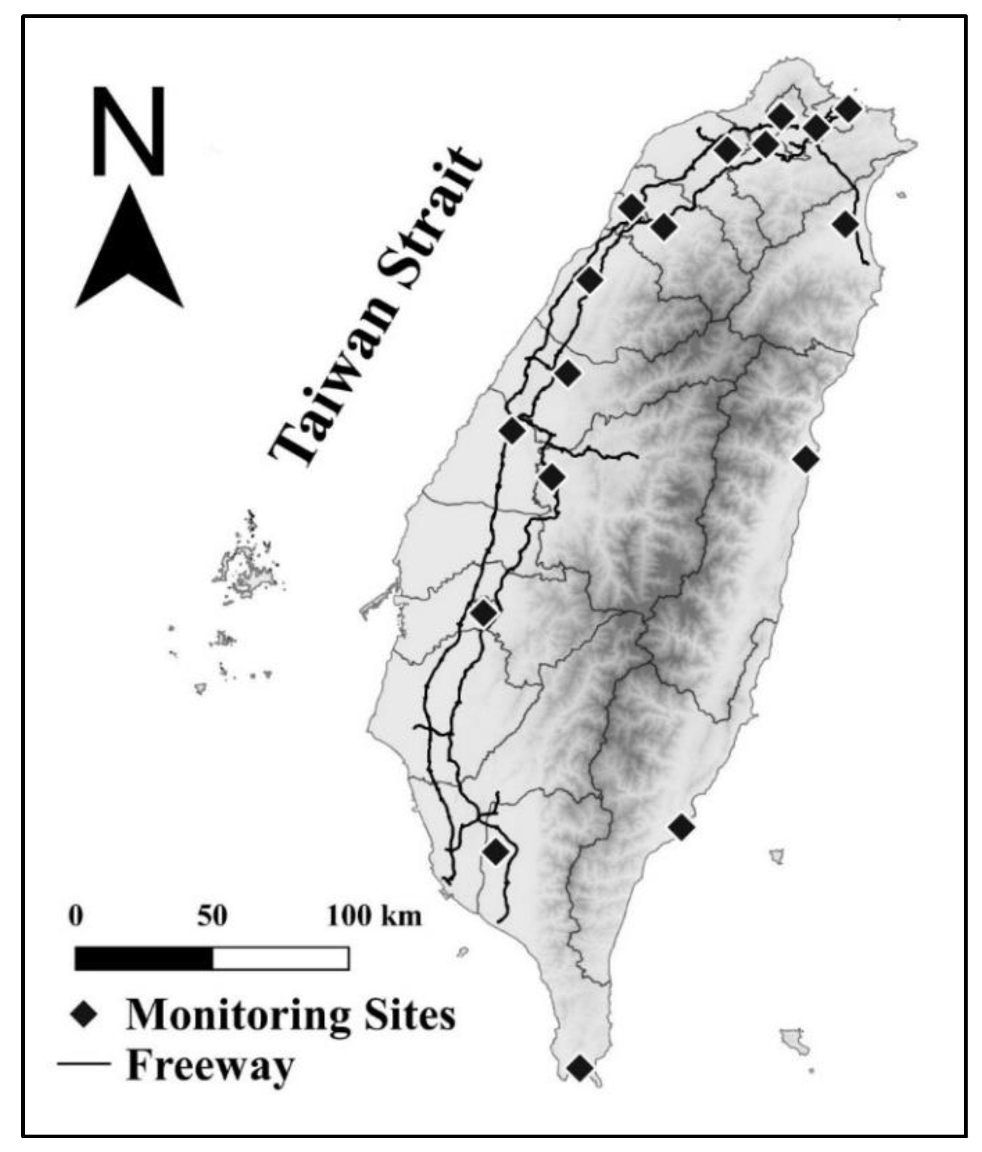
2.1. PM2.5 Sample Collection and Chemical Analysis

Filter-based PM2.5 samples used in this study were collected in Taiwan, which has an approximate population of 23 million and an area of 36,000 km2. Here, 24 daily samples (two samples per month per site in 2014) from 17 air quality monitoring sites, total 408 samples, were obtained from Taiwan Environmental Protection Administration (TEPA) (www.epa.gov.tw) and applied for chemical analysis. Figure 1 shows the locations of sites.
A total of 11 elemental composition, including Al, Ca, Cr, Fe, K, Mn, S, Si, Ti, V, and Zn, were quantitatively obtained using energy-dispersive X-ray fluorescence spectrometry with a high detection rate (≥70%) [15]. Calibration curves were built using thin-film standards (Micromatter, Vancouver, Canada). National Institute of Standards and Technology standard reference material (SRM 2783) was used to verify the measurements (Table S1). Furthermore, the method detection limit was computed as triple the standard deviation of the detected signals of each element in 10 blank Teflon filters. A multi-elemental quality control standard (Micromatter, Vancouver, BC, Canada) was analyzed for each batch of samples to ensure instrument performance.

2.2. Collection of LUR Predictors

For developing models, this study collected diverse potential predictors, including land use, road information, elevation, demographic data, location of stationary emission sources (e.g., factories and boilers), temples, and satellite data. A total of 21 predictor variables were created: area of road, residence, industry, port, semi-natural, and forest and urban green; length of road and distance to road; number of population, household, emission sources, and temples; extracted AOD values. The predictor variables are similar to the ones in our previous study and can be found elsewhere [24]. For detailed information of predictors, please see Table S2 of Supplementary Materials. The predictor variables applied in this study were processed and extracted using Quantum GIS 2.8.9 (QGIS) [25].
In this study, satellite-derived predictor of AOD was introduced in LUR model constructions to assess the efficacy for estimating concentrations of PM2.5 and the elemental composition. Larger AOD values indicate a hazier condition and higher aerosol concentration in atmosphere. The daily AOD acquired in this study were measured by moderate resolution imaging spectroradiometers (MODIS) onboard Terra and Aqua satellites via the principle of optical properties of aerosol (e.g., extinction or backscatter). AOD in spatial resolution of 3 km × 3 km were retrieved from MODIS aerosol products of MOD04_3K and MYD04_3K. Average AOD were computed from the 3 × 3 group (i.e., a 9 km × 9 km area centered at each air quality monitoring site) to reduce the effects of having missing AOD value at the center pixel. To further utilize the AOD data, an additional predictor, the AOD percentage (AOD_PER), was calculated based on the following formula:
Daily   AOD _ PER = number   of   pixels   with   available   AOD   9   ( total   number   of   pixels )
Daily AOD is calculated as an average of Terra and Aqua AOD values. Annual averages of AOD and AOD_PER were computed based on 365 daily values for modeling.

2.3. Model Constructions

LUR is built with a supervised stepwise selection procedure [12] using SAS statistical software (SAS 9.4; SAS Institute Inc., Cary, NC, USA). The construction procedure is described concisely as follows. Firstly, the start model was chosen as the univariate linear regression model with the highest adjusted explained variance (adjusted R2). Next, remaining predictors were sequentially regressed against the start model and the predictor was retained if the criteria were all achieved: (a) has the highest improved adjusted R2 (also > 0.01), (b) direction of coefficient matched with the anticipated effect, and (c) directions of remaining predictors were unchanged. Then, the predictors with p-value higher than 0.10 were removed after no more predictors met the above criteria. For predictors with variance inflation factor (VIF) > 3, the one with the highest VIF value was excluded to minimize the collinearity effects. Cook’s D and Moran’s I were utilized for evaluating influential sites and spatial autocorrelations. LUR model performance was assessed by leave-one-out cross-validation (LOOCV) and root mean square error (RMSE).
In this study, three methods were assessed for annual LUR model constructions. For Method 1, non-satellite predictors, including land use, road information, elevation, demographic data, stationary emission sources, and temples were applied for model building. For Method 2, AOD was added to the aforementioned predictors in Method 1. For Method 3, AOD_PER was introduced to the former predictors in Method 2. In addition, two scenarios defined as “high PM2.5 season” (HPS) and “low PM2.5 season” (LPS), classified by the period with PM2.5 concentration higher or lower than the average value, were developed using Method 3 for sensitivity analysis.

3. Results and Discussion

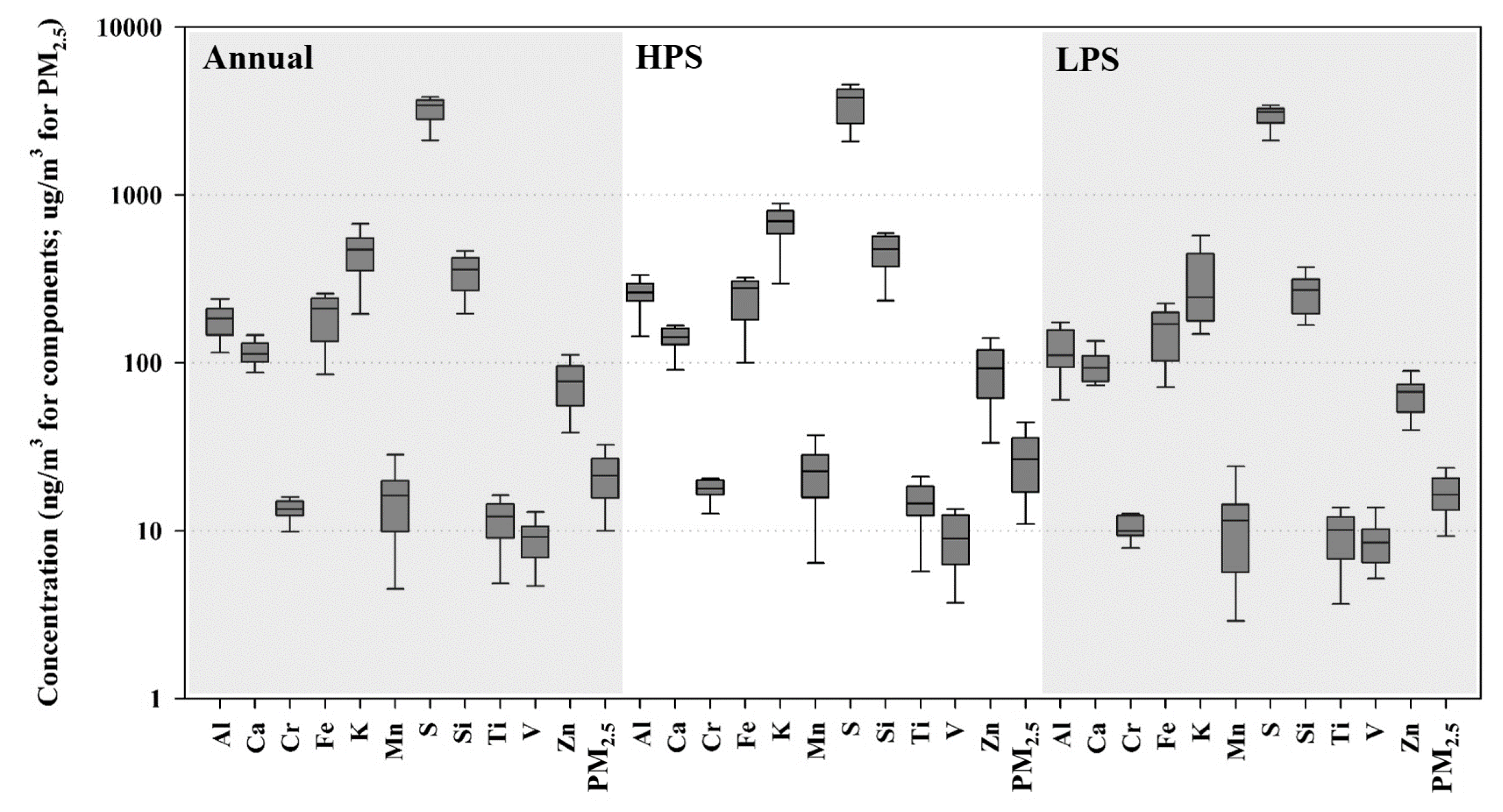
3.1. Summary Statistics of PM Measures

Figure 2 and Table S3 show the concentration distributions of PM2.5 and elemental composition in annual, HPS and LPS averages. For PM2.5, the annual concentration was 21.0 μg/m3. Among the compositions, S showed the highest annual concentration (3164.4 ng/m3), followed by K (448.5 ng/m3) and Si (343.7 ng/m3), whereas V exhibited the lowest value (9.0 ng/m3). Annual concentrations among other composition ranged from 11.5 to 191.9 ng/m3. The mean concentrations of PM measures are generally 1.0–1.5 times and 0.7–1.0 times as annual averages in HPS and LPS, respectively.

3.2. LUR Modeling Results

Among the three methods for constructing annual LUR models, Method 3 (considering AOD and AOD_PER as predictors) showed the best overall performance (median LOOCV R2 = 0.70) than Methods 1 and 2 (median LOOCV R2 = 0.37 and 0.44, respectively) (Table 1). Compared with the temporal-invariant land use predictors, satellite AOD and AOD_PER vary with time. Although their average values corresponding to the specific periods (i.e., annual, HPS, or LPS) were used in the models, they still are useful for representing the underlying variation of PM measures over time and space. Given the length restrictions of a technical note, we only discuss the main results of Method 3. For the summary of LUR models developed based on Methods 1 and 2, please refer to Tables S4 and S5 of Supplementary Materials.
Table 2 shows the annual model performances of PM2.5 and elemental composition from Method 3. LOOCV R2 among 12 PM measures ranged from 0.07 (V and Cr) to 0.92 (Si). Most PM measures, including PM2.5, Ca, Fe, K, Mn, S, Si, Ti, and Zn, showed LOOCV R2 higher than 0.40, indicating reasonable performance of the constructed LUR models. The length and surface area of road network and distance to road were applied in LUR development to represent traffic factors. Ca, Fe, Si, Ti, and Zn retained road-related predictors in the final models. Ca, Fe, Si, and Ti are regarded as crustal elements and roadside dust, which may be re-suspended by wind flow and heavy traffic [26,27,28]. Fe and Zn may be contributed by the abrasion of tire wear or brake linings from automobiles [29,30,31].
INDUSTRY (industrial area in buffer size (i.e., radius) of 1000 or 5000 m) and number of stationary emission sources (POINT_N_5000) were selected in the models of PM2.5, Cr, Fe, K, Mn, Si, Ti, and Zn. Cr, Fe, K, Mn, and Zn may be emitted from the ferrous or non-ferrous metal processing of industrial sources [32,33,34]. Si and Ti belong to crustal elements and are commonly utilized as markers of soil or construction dusts [35], and may also present in the industrial process of cement production or metal manufacturing [33,36,37]. Besides, the large buffer size (5000 m) implied that the elemental composition were influenced by distant industrial sources. Comparing with the studies conducted in Taipei and Kaohsiung in Taiwan, the industrial area variables were also retained in the final LUR models for PM2.5, Fe, Mn, Si, Ti, and Zn [15,38].
In this study, the number of temples was considered as a culture-specific predictor in model constructions. Five composition, K, S, Si, Ti, and V, retained the variable of temples in the final models. This variable was not significant in Hsu et al. [17], possibly because the limited number of monitoring sites in that study did not reflect the variabilities of environmental information. More geographically heterogeneous sites are expected to be included in LUR modeling for sufficiently representing the features of study areas.
Satellite-derived predictor of AOD was selected in four models among 12 PM measures (Table 1), including PM2.5, Fe, S, and Zn. AOD_PER was retained in nine models of PM2.5, Cr, Fe, K, Mn, S, Si, Ti, and Zn. LOOCV R2 of most PM measures increased significantly after AOD and AOD_PER were introduced in modeling, as compared to results from Method 1. For PM2.5, Fe, K, Mn, S, Si, Ti, and Zn, LOOCV R2 increased more than 0.30. AOD and AOD_PER exhibited a strong Pearson correlation with PM2.5 (0.75 with AOD; 0.69 with AOD_PER) and specific elemental composition (ranged from 0.69 to 0.72 with AOD; 0.35 to 0.74 with AOD_PER), and thus beneficial for the construction of spatial prediction model. AOD is obtained through measuring the extinction of the solar beam by particles, which relates to the amount of suspended aerosol in atmosphere. However, LOOCV R2 of Al and Cr model decreased. Predictor selection procedures were examined, which indicated that the presence of AOD or AOD_PER affected the selection procedures and changed the results. Thus, the model did not always give superior performance as more predictors were considered in model constructions.
AOD_PER showed positive coefficients in all nine LUR models. The value of AOD_PER depends on the availability of AOD, which is mainly influenced by cloud cover effect. Higher AOD_PER indicates fewer missing values and therefore less cloud cover effects, leading to the lower possibilities of precipitation and higher potentials of photochemical reaction from solar radiation. Precipitation reduces PM2.5 concentration in the atmosphere and corresponds with the decrease of elemental composition in PM2.5 mixtures while the photochemical reaction partially contributes to the formation of secondary aerosol. Furthermore, the fine particulate matters with higher hygroscopicity potentially facilitate the cloud formation which is related to AOD_PER value, indicating that the AOD_PER parameter includes the information of aerosol type.
In this study, the samples were divided into HPS and LPS based on PM2.5 levels higher or lower than the average value (=21.0 μg/m3) and LUR models were built accordingly using Method 3 (Tables S6 and S7). January to April and December were classified as the HPS while May to November as the LPS. The average temperature during the HPS and LPS was 18.7 vs. 28.1 °C, respectively (Figure S1). During the cold season, the lower mixing height would be favorable to form high air pollutions [39]. Overall, the model performed better during the HPS than during the LPS (Table 1, median LOOCV R2 = 0.76 vs. 0.46). Additionally, AOD_PER showed higher occurrences in HPS models than in LPS models. AOD_PER represents an indirect indicator of cloud coverage, implying that meteorological factors might be decisive predictors and more critical to estimate the levels of PM2.5 and associated elemental composition during the HPS than the LPS. Moreover, Al, Ca, and Mn showed better LOOCV R2 in both HPS and LPS models than in the annual models. This suggests that predictors might have different effects on certain PM measures by seasons, which cannot be reflected in annual models. For example, AOD_PER was retained in the HPS model but not annual model for Al. This may be because the meteorological variability was smoothed out in annual averages, thus cannot reflect the seasonal variance of Al level by AOD_PER.
For applications in epidemiological studies, most previous studies considered LOOCV R2 greater than 0.40 as an inclusion criterion [40,41,42,43]. Table 1 shows that the number of applicable models (LOOCV R2 > 0.40) was nine (Method 3) for the annual data, and increased to 12 for HPS. It was also noted that the LOOCV R2 of Al, Cr, and V improved significantly from < 0.3 in the annual models to 0.70, 0.62, and 0.53, respectively, in HPS models. This suggests potential influence of diverse meteorological conditions between clean and hazy days. Further investigation is needed to explore the meteorological effect to the LUR modeling. One limitation of this study is that the models are not applicable to mountainous areas since the locations of samples were mainly distributed at altitude < 250 m.

4. Conclusions

In this technical note, the efficacy of developing LUR models for PM2.5 and elemental composition with satellite-derived AOD was evaluated. The LOOCV R2 for all PM measures were higher than 0.40, except for Al, Cr, and V, after including AOD and AOD_PER, indicating the critical improvements for model constructions. In HPS models, LOOCV R2 of Al, Cr, and V significantly increased and were higher than 0.40, demonstrating the improved utility of the models during hazy periods.

Supplementary Materials

The following are available online at https://www.mdpi.com/article/10.3390/atmos12081018/s1, Table S1: Certified and measured values for PM measures using National Institute of Standards and Technology Standard Reference Material 2783 (n = 3), Table S2: The definitions of predictor variables in constructions of LUR models, Table S3: Descriptive statistics of PM2.5 and elemental composition in annual value, HPS and LPS, Table S4: Summary of land use regression models of PM2.5 and elemental composition using annual averages (Method 1), Table S5: Summary of land use regression models of PM2.5 and elemental composition using annual averages (Method 2), Table S6: Summary of land use regression models of PM2.5 and elemental composition in high PM2.5 season (HPS) (Method 3), Table S7: Summary of land use regression models of PM2.5 and elemental composition in low PM2.5 season (LPS) (Method 3), Figure S1: Comparison of monthly PM2.5 concentration (black column) and ambient temperature (dotted line).

Funding

This study was funded by National Taiwan University (105R7812) and the ‘Innovation and Policy Center for Population Health and Sustainable Environment (Population Health Research Center, PHRC), College of Public Health, National Taiwan University’ from The Featured Areas Research Center Program within the framework of the Higher Education Sprout Project by the Ministry of Education of Taiwan (NTU-107L9003).

Institutional Review Board Statement

Not applicable.

Informed Consent Statement

Not applicable.

Data Availability Statement

The data availability and collection are described in Material and Methods and Table S2 of Supplementary Materials.

Acknowledgments

We thank Taiwan Environmental Protection Administration for providing PM2.5 filter samples.

Conflicts of Interest

The authors declare no conflict of interest.

References

  1. Pope, C.A., III; Dockery, D.W. Health effects of fine particulate air pollution: Lines that connect. J. Air Waste Manag. Assoc. 2006, 56, 709–742. [Google Scholar] [CrossRef] [PubMed]
  2. Kampa, M.; Castanas, E. Human health effects of air pollution. Environ. Pollut. 2008, 151, 362–367. [Google Scholar] [CrossRef] [PubMed]
  3. Seagrave, J.; McDonald, J.D.; Bedrick, E.; Edgerton, E.S.; Gigliotti, A.P.; Jansen, J.J.; Ke, L.; Naeher, L.P.; Seilkop, S.K.; Zheng, M.; et al. Lung Toxicity of Ambient Particulate Matter from Southeastern U.S. Sites with Different Contributing Sources: Relationships between Composition and Effects. Environ. Health Perspect. 2006, 114, 1387–1393. [Google Scholar] [CrossRef] [Green Version]
  4. Pedersen, M.; Stayner, L.; Slama, R.; Sørensen, M.; Figueras, F.; Nieuwenhuijsen, M.J.; Raaschou-Nielsen, O.; Dadvand, P. Ambient Air Pollution and Pregnancy-Induced Hypertensive Disorders. Hypertension 2014, 64, 494–500. [Google Scholar] [CrossRef] [Green Version]
  5. Kelly, F.J.; Fussell, J.C. Size, source and chemical composition as determinants of toxicity attributable to ambient particulate matter. Atmospheric Environ. 2012, 60, 504–526. [Google Scholar] [CrossRef]
  6. Stanek, L.W.; Sacks, J.D.; Dutton, S.J.; Dubois, J.-J.B. Attributing health effects to apportioned components and sources of particulate matter: An evaluation of collective results. Atmospheric Environ. 2011, 45, 5655–5663. [Google Scholar] [CrossRef]
  7. Thurston, G.D.; Burnett, R.T.; Turner, M.C.; Shi, Y.; Krewski, D.; Lall, R.; Ito, K.; Jerrett, M.; Gapstur, S.M.; Diver, W.R.; et al. Ischemic Heart Disease Mortality and Long-Term Exposure to Source-Related Components of U.S. Fine Particle Air Pollution. Environ. Health Perspect. 2016, 124, 785–794. [Google Scholar] [CrossRef] [PubMed] [Green Version]
  8. Achilleos, S.; Kioumourtzoglou, M.-A.; Wu, C.-D.; Schwartz, J.D.; Koutrakis, P.; Papatheodorou, S.I. Acute effects of fine particulate matter constituents on mortality: A systematic review and meta-regression analysis. Environ. Int. 2017, 109, 89–100. [Google Scholar] [CrossRef]
  9. Yang, J.; Zhou, M.; Li, M.; Yin, P.; Hu, J.; Zhang, C.; Wang, H.; Liu, Q.; Wang, B. Fine particulate matter constituents and cause-specific mortality in China: A nationwide modelling study. Environ. Int. 2020, 143, 105927. [Google Scholar] [CrossRef]
  10. Hoek, G.; Beelen, R.; De Hoogh, K.; Vienneau, D.; Gulliver, J.; Fischer, P.; Briggs, D. A review of land-use regression models to assess spatial variation of outdoor air pollution. Atmospheric Environ. 2008, 42, 7561–7578. [Google Scholar] [CrossRef]
  11. ESCAPE. ESCAPE Exposure Assessment Manual. Available online: http://www.escapeproject.eu/manuals/ESCAPE_Exposure-manualv9.pdf (accessed on 26 January 2019).
  12. Eeftens, M.; Beelen, R.; De Hoogh, K.; Bellander, T.; Cesaroni, G.; Cirach, M.; Declercq, C.; Dėdelė, A.; Dons, E.; de Nazelle, A.; et al. Development of Land Use Regression Models for PM2.5, PM2.5 Absorbance, PM10 and PMcoarse in 20 European Study Areas; Results of the ESCAPE Project. Environ. Sci. Technol. 2012, 46, 11195–11205. [Google Scholar] [CrossRef]
  13. Lee, J.-H.; Wu, C.-F.; Hoek, G.; de Hoogh, K.; Beelen, R.; Brunekreef, B.; Chan, C.-C. Land use regression models for estimating individual NOx and NO2 exposures in a metropolis with a high density of traffic roads and population. Sci. Total. Environ. 2014, 472, 1163–1171. [Google Scholar] [CrossRef]
  14. Wu, C.-D.; Chen, Y.-C.; Pan, W.-C.; Zeng, Y.-T.; Chen, M.-J.; Guo, Y.L.; Lung, S.-C.C. Land-use regression with long-term satellite-based greenness index and culture-specific sources to model PM2.5 spatial-temporal variability. Environ. Pollut. 2017, 224, 148–157. [Google Scholar] [CrossRef]
  15. Wu, C.-F.; Lin, H.-I.; Ho, C.-C.; Yang, T.-H.; Chen, C.-C.; Chan, C.-C. Modeling horizontal and vertical variation in intraurban exposure to PM2.5 concentrations and compositions. Environ. Res. 2014, 133, 96–102. [Google Scholar] [CrossRef] [PubMed]
  16. de Hoogh, K.; Wang, M.; Adam, M.; Badaloni, C.; Beelen, R.; Birk, M.; Cesaroni, G.; Cirach, M.; Declercq, C.; Dėdelė, A.; et al. Development of Land Use Regression Models for Particle Composition in Twenty Study Areas in Europe. Environ. Sci. Technol. 2013, 47, 5778–5786. [Google Scholar] [CrossRef]
  17. Hsu, C.-Y.; Wu, C.-D.; Hsiao, Y.-P.; Chen, Y.-C.; Chen, M.-J.; Lung, S.-C.C. Developing Land-Use Regression Models to Estimate PM2.5—Bound Compound Concentrations. Remote Sens. 2018, 10, 1971. [Google Scholar] [CrossRef] [Green Version]
  18. Ito, K.; Johnson, S.; Kheirbek, I.; Clougherty, J.; Pezeshki, G.; Ross, Z.; Eisl, H.; Matte, T.D. Intraurban Variation of Fine Particle Elemental Concentrations in New York City. Environ. Sci. Technol. 2016, 50, 7517–7526. [Google Scholar] [CrossRef] [PubMed]
  19. Tunno, B.J.; Shmool, J.L.; Michanowicz, D.R.; Tripathy, S.; Chubb, L.; Kinnee, E.; Cambal, L.; Roper, C.; Clougherty, J.E. Spatial variation in diesel-related elemental and organic PM2.5 components during workweek hours across a downtown core. Sci. Total. Environ. 2016, 573, 27–38. [Google Scholar] [CrossRef] [Green Version]
  20. Brokamp, C.; Jandarov, R.; Rao, M.; LeMasters, G.; Ryan, P. Exposure assessment models for elemental components of particulate matter in an urban environment: A comparison of regression and random forest approaches. Atmospheric Environ. 2017, 151, 1–11. [Google Scholar] [CrossRef] [PubMed] [Green Version]
  21. Dirgawati, M.; Heyworth, J.; Wheeler, A.; McCaul, K.A.; Blake, D.; Boeyen, J.; Cope, M.; Yeap, B.B.; Nieuwenhuijsen, M.; Brunekreef, B.; et al. Development of Land Use Regression models for particulate matter and associated components in a low air pollutant concentration airshed. Atmospheric Environ. 2016, 144, 69–78. [Google Scholar] [CrossRef]
  22. Chen, J.; De Hoogh, K.; Gulliver, J.; Hoffmann, B.; Hertel, O.; Ketzel, M.; Weinmayr, G.; Bauwelinck, M.; Van Donkelaar, A.; Hvidtfeldt, U.A.; et al. Development of Europe-Wide Models for Particle Elemental Composition Using Supervised Linear Regression and Random Forest. Environ. Sci. Technol. 2020, 54, 15698–15709. [Google Scholar] [CrossRef] [PubMed]
  23. Tripathy, S.; Tunno, B.J.; Michanowicz, D.R.; Kinnee, E.; Shmool, J.L.; Gillooly, S.; Clougherty, J.E. Hybrid land use regression modeling for estimating spatio-temporal exposures to PM2.5, BC, and metal components across a metropolitan area of complex terrain and industrial sources. Sci. Total. Environ. 2019, 673, 54–63. [Google Scholar] [CrossRef]
  24. Huang, C.-S.; Lin, T.-H.; Hung, H.; Kuo, C.-P.; Ho, C.-C.; Guo, Y.-L.; Chen, K.-C.; Wu, C.-F. Incorporating satellite-derived data with annual and monthly land use regression models for estimating spatial distribution of air pollution. Environ. Model. Softw. 2019, 114, 181–187. [Google Scholar] [CrossRef]
  25. QGIS Development Team. QGIS Geographic Information System. Available online: https://qgis.osgeo.org (accessed on 16 April 2019).
  26. Gugamsetty, B.; Wei, H.; Liu, C.-N.; Awasthi, A.; Hsu, S.-C.; Tsai, C.-J.; Roam, G.-D.; Wu, Y.-C.; Chen, C.-F. Source Characterization and Apportionment of PM10, PM2.5 and PM0.1 by Using Positive Matrix Factorization. Aerosol Air Qual. Res. 2012, 12, 476–491. [Google Scholar] [CrossRef]
  27. Liu, W.; Wang, Y.; Russell, A.; Edgerton, E.S. Atmospheric aerosol over two urban–rural pairs in the southeastern United States: Chemical composition and possible sources. Atmospheric Environ. 2005, 39, 4453–4470. [Google Scholar] [CrossRef]
  28. Vallius, M.; Lanki, T.; Tiittanen, P.; Koistinen, K.; Ruuskanen, J.; Pekkanen, J.; Vallius, M.; Lanki, T.; Tiittanen, P.; Koistinen, K.; et al. Source apportionment of urban ambient PM2.5 in two successive measurement campaigns in Helsinki, Finland. Atmospheric Environ. 2003, 37, 615–623. [Google Scholar] [CrossRef]
  29. Sternbeck, J.; Sjödin, Å.; Andréasson, K. Metal emissions from road traffic and the influence of resuspension—Results from two tunnel studies. Atmospheric Environ. 2002, 36, 4735–4744. [Google Scholar] [CrossRef]
  30. Hjortenkrans, D.; Bergbäck, B.; Häggerud, A. New Metal Emission Patterns in Road Traffic Environments. Environ. Monit. Assess. 2006, 117, 85–98. [Google Scholar] [CrossRef]
  31. Birmili, W.; Allen, A.G.; Bary, F.; Harrison, R.M. Trace Metal Concentrations and Water Solubility in Size-Fractionated Atmospheric Particles and Influence of Road Traffic. Environ. Sci. Technol. 2006, 40, 1144–1153. [Google Scholar] [CrossRef]
  32. Heo, J.-B.; Hopke, P.; Yi, S.-M. Source apportionment of PM2.5 in Seoul, Korea. Atmospheric Chem. Phys. Discuss. 2009, 9, 4957–4971. [Google Scholar] [CrossRef] [Green Version]
  33. Han, J.S.; Moon, K.J.; Lee, S.J.; Kim, Y.J.; Ryu, S.Y.; Cliff, S.S.; Yi, S.M. Size-resolved source apportionment of ambient particles by positive matrix factorization at Gosan background site in East Asia. Atmospheric Chem. Phys. Discuss. 2006, 6, 211–223. [Google Scholar] [CrossRef] [Green Version]
  34. Lee, J.H.; Hopke, P.K. Apportioning sources of PM2.5 in St. Louis, MO using speciation trends network data. Atmospheric Environ. 2006, 40, 360–377. [Google Scholar] [CrossRef]
  35. Du, W.; Hong, Y.-W.; Xiao, H.; Zhang, Y.; Chen, Y.; Xu, L.; Chen, J.; Deng, J. Chemical Characterization and Source Apportionment of PM2.5 during Spring and Winter in the Yangtze River Delta, China. Aerosol Air Qual. Res. 2017, 17, 2165–2180. [Google Scholar] [CrossRef]
  36. Dimitriou, K.; Remoundaki, E.; Mantas, E.; Kassomenos, P. Spatial distribution of source areas of PM2.5 by Concentration Weighted Trajectory (CWT) model applied in PM2.5 concentration and composition data. Atmospheric Environ. 2015, 116, 138–145. [Google Scholar] [CrossRef]
  37. Liu, B.; Song, N.; Dai, Q.; Mei, R.; Sui, B.; Bi, X.; Feng, Y. Chemical composition and source apportionment of ambient PM2.5 during the non-heating period in Taian, China. Atmospheric Res. 2016, 170, 23–33. [Google Scholar] [CrossRef]
  38. Ho, C.-C.; Chan, C.-C.; Cho, C.-W.; Lin, H.-I.; Lee, J.-H.; Wu, C.-F. Land use regression modeling with vertical distribution measurements for fine particulate matter and elements in an urban area. Atmospheric Environ. 2015, 104, 256–263. [Google Scholar] [CrossRef]
  39. Yu, T.-Y.; Chang, I.-C. Spatiotemporal Features of Severe Air Pollution in Northern Taiwan (8 pp). Environ. Sci. Pollut. Res. 2006, 13, 268–275. [Google Scholar] [CrossRef]
  40. Adam, M.; Schikowski, T.; Carsin, A.E.; Cai, Y.; Jacquemin, B.; Sanchez, M.; Vierkötter, A.; Marcon, A.; Keidel, D.; Sugiri, D.; et al. Adult lung function and long-term air pollution exposure. ESCAPE: A multicentre cohort study and meta-analysis. Eur. Respir. J. 2014, 45, 38–50. [Google Scholar] [CrossRef] [Green Version]
  41. Chen, S.-Y.; Wu, C.-F.; Lee, J.-H.; Hoffmann, B.; Peters, A.; Brunekreef, B.; Chu, D.-C.; Chan, C.-C. Associations between Long-Term Air Pollutant Exposures and Blood Pressure in Elderly Residents of Taipei City: A Cross-Sectional Study. Environ. Health Perspect. 2015, 123, 779–784. [Google Scholar] [CrossRef]
  42. Morgenstern, V.; Zutavern, A.; Cyrys, J.; Brockow, I.; Gehring, U.; Koletzko, S.; Bauer, C.P.; Reinhardt, D.; Wichmann, H.-E.; Heinrich, J. Respiratory health and individual estimated exposure to traffic-related air pollutants in a cohort of young children. Occup. Environ. Med. 2006, 64, 8–16. [Google Scholar] [CrossRef] [Green Version]
  43. Wolf, K.; Stafoggia, M.; Cesaroni, G.; Andersen, Z.J.; Beelen, R.; Galassi, C.; Hennig, F.; Migliore, E.; Penell, J.; Ricceri, F.; et al. Long-term Exposure to Particulate Matter Constituents and the Incidence of Coronary Events in 11 European Cohorts. Epidemiology 2015, 26, 565–574. [Google Scholar] [CrossRef] [PubMed] [Green Version]
Figure 1. Locations of 17 selected TEPA monitoring sites including in this study.
Atmosphere 12 01018 g001
Figure 2. Concentration distributions of PM measures for annual value, high PM2.5 season (HPS) and low PM2.5 season (LPS) (the box represents 25th–75th percentiles and median, and the whiskers represent 10th and 90th percentiles) (N = 17).
Atmosphere 12 01018 g002
Table 1. LOOCV R2 and selected satellite-derived predictors among land use regression models based on different methods.
PM
Measures
Annual Model: Evaluating AOD and AOD_PER Efficacy in LURScenario 1:
High PM2.5 Season (HPS)
Scenario 2:
Low PM2.5 Season (LPS)
Method 1:
Base
Method 2:
Base + AOD
Method 3:
Base + AOD + AOD_PER
Method 3:
Base + AOD + AOD_PER
Method 3:
Base + AOD + AOD_PER
LOOCV R2LOOCV R2AOD aLOOCV R2AODAOD_PER aLOOCV R2AODAOD_PERLOOCV R2AODAOD_PER
PM2.50.350.44Y0.69YY0.91YY0.40Y
Al0.330.44Y0.26 0.70 Y0.55Y
Ca0.580.58 0.58 0.73 Y0.59
Cr0.240.24 0.07 Y0.62 Y0.29 Y
Fe0.400.63Y0.77YY0.80 Y0.43Y
K0.400.30Y0.71 Y0.67 Y0.33Y
Mn0.050.70Y0.69 Y0.90 Y0.80Y
S0.340.40Y0.86YY0.87 Y0.36Y
Si0.390.47Y0.92 Y0.49 Y0.76 Y
Ti0.410.41 0.80 Y0.86 Y0.49 Y
V0.070.07 0.07 0.53 Y0.07
Zn0.440.57Y0.83YY0.91 Y0.71 Y
Mean0.330.44 0.60 0.75 0.48
Median0.370.44 0.70 0.76 0.46
>0.40 b59 9 12 8
a Represents whether AOD or AOD_PER was retained in the final model. “Y” denotes Yes. b Represents the number of models higher than LOOCV R2 of 0.40.
Table 2. Summary of land use regression models of PM2.5 and elemental composition using annual averages (Method 3).
PM MeasuresLUR Model aR2 of ModelAdjusted R2LOOCV R2LOOCV RMSE bp-Value of Moran’s I
PM2.5−1.05 − 542.39 × URBANGREEN_100 + 0.03 × POINT_N_5000 + 23.71 × AOD + 120.10 × AOD_PER0.840.780.694.280.43
Al145.24 + 1061.16 × URBANGREEN_5000.400.360.2639.930.57
Ca76.97 + 457.55 × MAJORRAODAREA_500 + 96.48 × MAJORROADLEN_1000.700.660.5814.020.58
Cr12.26 + 6.22 × INDUSTRY_1000 − 155.46 × SEMINATURAL + 16.86 × AOD_PER0.540.440.071.900.12
Fe−30.58 + 1230.54 × MAJORROADAREA_500 − 5168.54 × URBANGREEN_100 + 0.25 × POINT_N_5000 + 275.39 × AOD + 595.94 × AOD_PER0.870.810.7732.440.46
K78.31 − 8741.33 × URBANGREEN_100 + 0.49 × POINT_N_5000 + 0.66 × TEMPLE_5000 + 3511.40 × AOD_PER0.880.850.7181.010.16
Mn2.36 + 54.86 × INDUSTRY_1000 + 0.02 × POINT_N_5000 + 106.78 × AOD_PER0.840.800.695.070.77
S1044.46 − 50105.99 × URBANGREEN_100 + 2.54 × HOUSEHOLD_5000 + 162.53 × TEMPLE_300 + 1585.70 × AOD + 14110.58 × AOD_PER0.920.880.86234.740.85
Si37.56 + 1406.59 × ALLROADAREA_300 + 37.15 × INDUSTRY_5000 − 11749.47 × URBANGREEN_100 + 9661.14 × DISTINVMR2 + 14.00 × TEMPLE_300 + 1977.17 × AOD_PER0.970.960.9229.290.77
Ti−0.88 + 6.50 × ALLROADAREA_1000 − 393.67 × URBANGREEN_100 + 0.01 × POINT_N_5000 + 0.03 × TEMPLE_5000 + 69.08× AOD_PER0.900.860.801.830.90
V7.25 + 1.62 × TEMPLE_3000.350.310.073.280.80
Zn−3.72 + 2750.53 × ALLROADAREA_100 + 43.53 × MAJORROADAREA_1000 + 7.12 × INDUSTRY_5000 − 2163.13 × URBANGREEN_100 + 66.32 × AOD + 277.57 × AOD_PER0.920.880.8310.480.76
a The surface area (km2) of all road (ALLROADAREA_X), major road (MAJORROADAREA_X), industry (INDUSTRY_X), urban green area (URBANGREEN_X), semi-natural and forested area (SEMINATURAL_X), the total length (km) of major roads (MAJORROADLEN_X), the number (N) of household (HOUSEHOLD_X), stationary emission sources (POINT_N_X), and temples (TEMPLE_X). The _X indicates the buffer size (in meters). DISTINVMR2 represents the inverse of distance squared to the nearest major road. AOD denotes the extracted AOD value at the site. AOD_PER denotes the AOD percentage at the site. b The concentration of PM2.5 and elemental composition are represented as μg/m3 and ng/m3, respectively.
Publisher’s Note: MDPI stays neutral with regard to jurisdictional claims in published maps and institutional affiliations.

