Observations of Atmospheric Aerosol and Cloud Using a Polarized Micropulse Lidar in Xi’an, China

Abstract

A polarized micropulse lidar (P-MPL) employing a pulsed laser at 532 nm was developed by the Institute of Oceanographic Instrumentation, Qilu University of Technology (Shandong Academy of Sciences). The optomechanical structure, technical parameters, detection principle, overlap factor calculation method, and inversion methods of the atmospheric boundary layer (ABL) depth and depolarization ratio (DR) were introduced. Continuous observations using the P-MPL were carried out at Xi’an Meteorological Bureau, and the observation data were analyzed. In this study, we gleaned much information on aerosols and clouds, including the temporal and spatial variation of aerosols and clouds, aerosol extinction coefficient, DR, and the structure of ABL were obtained by the P-MPL. The variation of aerosols and clouds before and after a short rainfall was analyzed by combining time-height-indication (THI) of range corrected signal (RCS) and DR was obtained by the P-MPL with profiles of potential temperature (PT) and relative humidity (RH) detected by GTS1 Digital Radiosonde. Then, the characteristics of tropopause cirrus cloud were discussed using the data of DR, PT, and RH. Finally, a haze process from January 1st to January 5th was studied by using aerosol extinction coefficients obtained by the P-MPL, PT, and RH profiles measured by GTS1 Digital Radiosonde and the time-varying of PM_2.5 and PM₁₀ observed by ambient air quality monitor. The source of the haze was simulated by using the NOAA HYSPLIT Trajectory Model.

1. Introduction

Atmospheric aerosols are microscopically small particles and mainly suspended in the lower troposphere [1,2]. They play an important role in the energy balance of the Earth system by directly scattering and absorbing solar radiation, and indirectly playing the role of cloud condensation nuclei (CCN) in cloud-forming processes. Accordingly, aerosol particles serving as CCN have a direct impact on cloud optical properties and rainfall probability [3,4,5]. In addition, the concentration and distribution of aerosols affect atmospheric visibility and public health by changing air quality [6,7]. With the development of urbanization and industrialization, air pollution is becoming more and more serious, and people pay more attention to air quality [8,9]. Therefore, it is important to study the optical properties and dynamics of aerosols.

Lidar (Light Detection and Ranging) is an active optical remote sensing device that has been proven to be a reliable tool for high temporal and spatial resolution remote sensing of atmospheric aerosols in real-time [10,11]. Knowledge of aerosol optical properties and distribution characteristics will help us to understand their role in atmospheric processes, as well as their effects on human health and the atmospheric environment. Using polarized lidar to observe the depolarization ratios (DR) and optical properties of atmospheric aerosols will make it possible to distinguish between types of aerosols and provide effective methods for the study of optical and microphysical properties of aerosols [12,13].

As early as 1971, Schotland et al., of New York University used polarized lidar to study the DR of cloud particles [14]. In 2006, the CALIPSO (Cloud-Aerosol Lidar and Infrared Pathfinder Satellite Observations) satellite was launched by the National Aeronautics and Space Administration (NASA) carrying a dual-wavelength (532 nm and 1064 nm) lidar for the study of global clouds and atmospheric aerosols. By using the 532 nm polarization channel to observe the polarization of global clouds and aerosols, satellite polarized lidar observation was realized [15]. Polarization measurement has become one of the standard configurations of atmospheric lidar, such as the micropulse lidar developed by Sigma Space Corporation of the United States, which has been used to observe volcanic ash [16].

A polarized micropulse lidar (P-MPL), designed and developed by the Institute of Oceanographic Instrumentation, Qilu University of Technology (Shandong Academy of Sciences) for measurements of aerosols and clouds in an automatic and continuous mode, was deployed at Xi’an Meteorological Bureau (34°18′ N, 108°56′ E) for operational observation. The purpose of the observation campaign is mainly to study the optical and polarization characteristics of urban aerosols and clouds. In this paper, the observation campaign is introduced firstly, and then the functions and specifications of the observation instruments, including the P-MPL, GTS1 Digital Radiosonde, and ambient air quality monitor are outlined. The detection principle of the P-MPL is discussed, while a geometric overlap factor calculation method, a DR calculation method, and an atmospheric boundary layer (ABL) depth inversion algorithm are proposed and tested in Section 3. Finally, some observation results in different weather conditions are presented and discussed.

2. Observation Campaign and Instruments

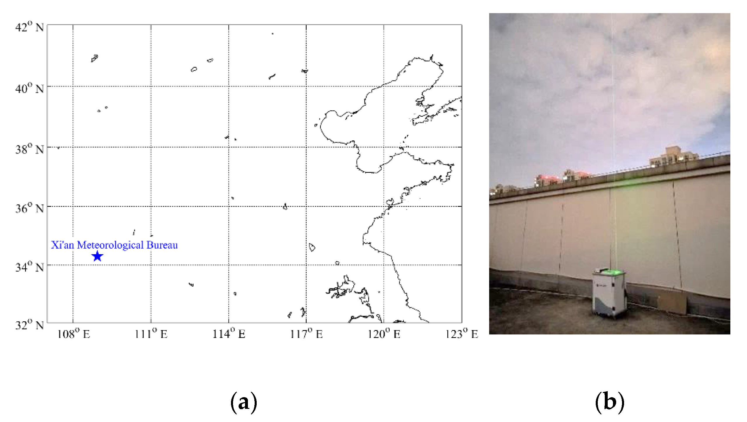
2.1. Observation Campaign in Xi’an

Xi’an is an important central city in Western China with a warm, temperate, semi-humid continental monsoon climate and with different features for each season. There are more rainy days in summer, while in winter, haze events occur frequently due to the influence factors of geographical location, meteorological conditions, and highway transportation. From June 2019 to April 2020, the P-MPL was operated automatically and continuously at Xi’an Meteorological Bureau (Figure 1), which is located in the urban area of Xi’an. The temporal and spatial distribution characteristics, optical characteristic parameters, and DR of atmospheric aerosols and clouds were obtained. In order to better understand the characteristics of aerosols and clouds in different weather conditions, the observational data of the P-MPL, GTS1 Digital Radiosonde and air quality monitor were used together for analysis.

2.2. The P-MPL Setup

The P-MPL with a depolarization-sensitive channel based on Mie scattering is developed for automatic observations of tropospheric aerosols and clouds. The structure of the P-MPL is shown in Figure 2 and the biaxial structure is adopted. A single wavelength (532 nm) pulsed laser emitting a Gaussian laser beam with single laser energy of 60 μJ, pulse length of 5 ns, and repetition frequency of 7 kHz as the transmitter is employed in the P-MPL. The backscattering signals are acquired by an 8-inch diameter aperture Schmidt–Cassegrain telescope. The signals collected by the telescope are further separated by a polarizing beam splitter (PBS) into parallel and perpendicular polarization components. Each component is measured separately by the parallel channel and perpendicular channel using photomultiplier tubes (PMTs). Finally, the data are recorded by a dual-channel photon counting card with a resolution of 250 ns, to which the corresponding range resolution of P-MPL is 37.5 m.

The specifications of the P-MPL are shown in

Table 1. The specifications of the P-MPL.

Parameters	Specification
Transmitter
Type	Diode-pumped solid state
Laser wavelength	532 nm
Pulse energy	60 µJ
Pulse duration	5 ns
Pulse repetition frequency	7 kHz
Beam divergence	200 µrad
Receiver
Telescope type	Schmidt–Cassegrain
Telescope diameter	8-inch
Field of view	500 µrad
Filter bandwidth	0.5 nm
Detector type	PMT
Detection mode	Photon counting
Range resolution	37.5 m
Detection range	0.1~20 km

.

2.3. GTS1 Digital Radiosonde

The GTS1 Digital Radiosonde is a relatively advanced digital high-altitude detector at present with the advantages of high precision, small volume, and high sensitivity. The strong anti-interference ability can ensure that it is not affected by the weather and the same frequency interference, and further ensure the stability and reliability of data acquisition and transmission. It is carried by hydrogen balloon, which is usually released at 7:15 and 19:15 local time every day. In the process of balloon rising, the meteorological elements such as temperature, humidity, wind, and pressure at different altitudes are measured. The main specifications of the GTS1 Digital Radiosonde are shown in

Table 2. The specifications of the GTS1 Digital Radiosonde.

Parameters	Specification
Temperature	−90 °C~50 °C
Relative humidity	0%~100%
Pressure	5 hPa~1060 hPa
Maximum detection altitude	36 km

. The range resolution of the digital radiosonde data used in this paper is 15 m.

2.4. Ambient Air Quality Monitor

Based on the principle of β-ray absorption, the ambient air quality monitor adopts a dual-channel structure and can simultaneously collect two kinds of pollution particles (PM_2.5 and PM₁₀) in the atmosphere, which can effectively reflect the variation of air pollution particle concentration. The specifications can be seen form

Table 3. The specifications of the ambient air quality monitor.

Parameters	Specification
Measuring range	0~1000 µg/m3
Minimum detection value	≤5 µg/m3
Minimum display unit	0.1 µg/m3
Sampling flow deviation	16.7 L/min ± 3%

.

3. Detection Principle and Data Processing Methods of the P-MPL

3.1. The Lidar Equation

The P-MPL emits a linearly polarized laser light and mainly uses the echo signals of parallel channel and perpendicular channel to study the atmospheric aerosols and clouds. For spherical aerosol particles, such as water droplets, the polarization planes of echo signals are oriented parallel to the outgoing beam. If the laser interacts with non-spherical aerosol particles (dust, ice crystals, etc.), the polarization planes of backscattering signals are no longer consistent with the polarization plane of the emitted laser beam; that is, depolarization occurs [17]. Generally, the lidar equations for the two polarization channels are shown as follows [18]:

$$P_p\left(r\right)=\frac{k_p{P}_0{A}_r{\beta }_p\left(r\right)}{r^2}exp\left[-2{{\displaystyle \int }}_0^r\alpha \left(r^{\prime }\right)d{r}^{\prime }\right]$$

(1)

$$P_s\left(r\right)=\frac{k_s{P}_0{A}_r{\beta }_s\left(r\right)}{r^2}exp\left[-2{{\displaystyle \int }}_0^r\alpha \left(r^{\prime }\right)d{r}^{\prime }\right]$$

(2)

where P(r) is the intensity of echo signal at the distance r, P₀ is the intensity of laser emission, A_r is the aperture area, α(r) is extinction coefficient, β(r) is the backscattering coefficient, and k is the lidar correction constant, which is related to geometric overlap factor, total transmittance, and range resolution. The subscript P and S represent parallel polarization and perpendicular polarization components, respectively.

The range corrected signal (RCS) is defined in Equation (3):

$$\mathrm{RCS}\left(r\right)=P\left(r\right)\cdot r^2$$

(3)

Both extinction coefficient and backscattering coefficient reflect the optical properties of the aerosol. Here, the extinction coefficient and backscattering coefficient are retrieved using the Fernald method [19], and the lidar ratio of urban aerosol is assumed to be 50 sr [20].

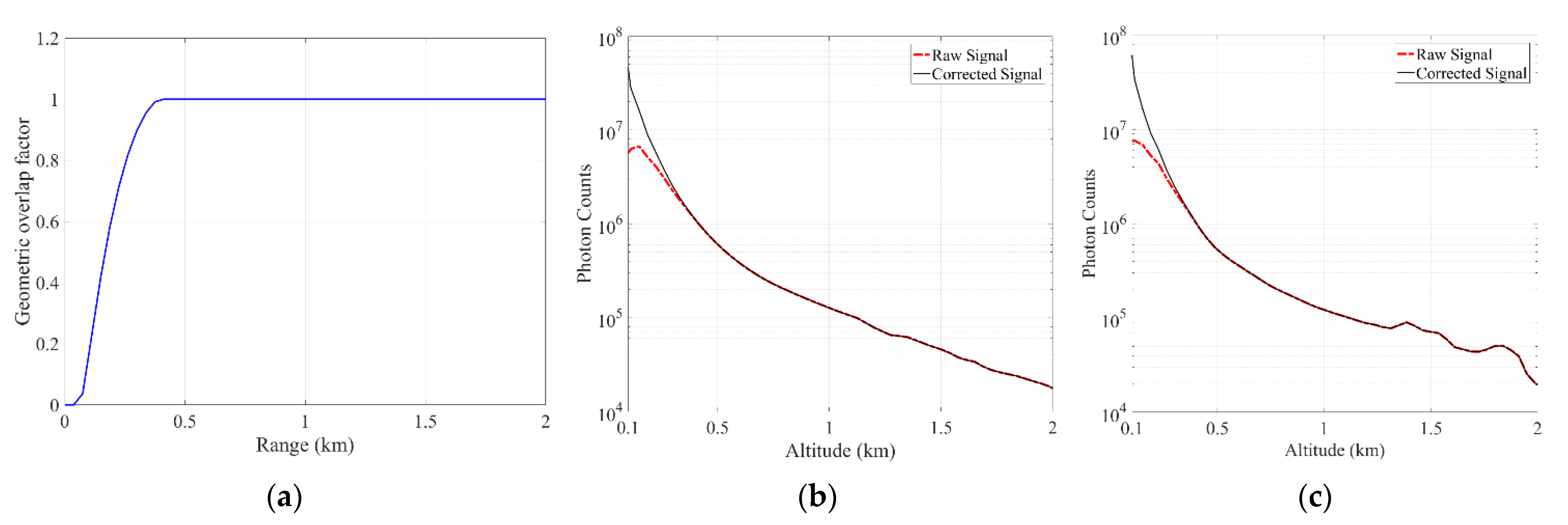
3.2. Geometric Overlap Factor Calculation Method

To better understand the near distance signal, the geometric overlap factor G(r) should be calculated. G(r) is defined as the ratio of laser beam energy P(r) to total energy P₀(r) in the field of view at range r in biaxial lidar [21]. Assuming that the laser energy is uniformly distributed, G(r) can be described by Equation (4):

$$G\left(r\right)=\frac{S_{\mathrm{overlap}}\left(r\right)}{S_L\left(r\right)}$$

(4)

where S_overlap(r) is the overlap area of the field of view and the laser beam area in range r, and S_L(r) is the laser beam area in range r. The G(r) changes with r and is shown in Figure 3. The altitude of G(r) = 0 is the detection blind area, where atmospheric echo data will not be received. The altitude of 0< G(r) < 1 is referred to as the transition zone, where only part of the data will be received. After passing the transition zone, the echo data will be completely received and G(r) = 1. Therefore, it is necessary to calculate G(r) to normalize the signal in the transition zone to the condition when G(r) = 1.

The main parameters for calculating G(r) in biaxial lidar include output beam diameter D_L, telescope diameter D_R, laser beam divergence angle θ_L, field of view θ_FOV, the transmitter-receiver separation D, and angle of misaligned optical axes ω.

The diameters of laser beam and the field of view of receiver changing with r are described in Equations (5) and (6):

$$D_L\left(r\right)=r\cdot {\theta }_L+D_L$$

(5)

$$D_R\left(r\right)=r\cdot {\theta }_{FOV}+D_R$$

(6)

If the optical axes of transmitter and receiver are misaligned, the transmitter-receiver separation also varies with r:

$$D\left(r\right)=D+\omega \cdot r$$

(7)

When ω is positive, it means that the optical axes of transmitter and receiver are separated, and when ω is negative, it indicates that the optical axes of transmitter and receiver are intersecting. If optics are slightly misaligned, for example $\omega <\frac{{\theta }_{FOV}}{2}-\frac{{\theta }_L}{2}$, above the blind area and transition area, the G(r) will be 1. If ω is larger, the long-distance beam plane will partially coincide with the field of view or completely separate from the field of view, and then affect the detection efficiency and signal accuracy of lidar. S_L(r) and S_overlap(r) are described in Equations (8) and (9):

$$S_L\left(r\right)=\pi \cdot {\left(\frac{D_L\left(r\right)}{2}\right)}^2$$

(8)

$$\begin{gathered} S_{\mathrm{overlap}}\left(r\right)={\left(\frac{D_L\left(r\right)}{2}\right)}^2\cdot arccos\left(\frac{{\left(\frac{D_L\left(r\right)}{2}\right)}^2+D{\left(r\right)}^2-{\left(\frac{D_R\left(r\right)}{2}\right)}^2}{D_L\left(r\right)\cdot D\left(r\right)}\right)-\frac{1}{2}\cdot {\left(\frac{D_L\left(r\right)}{2}\right)}^2\cdot sin\left(2\cdot \\ arccos\left(\frac{{\left(\frac{D_L\left(r\right)}{2}\right)}^2+D{\left(r\right)}^2-{\left(\frac{D_R\left(r\right)}{2}\right)}^2}{D_L\left(r\right)\cdot D\left(r\right)}\right)\right)+{\left(\frac{D_R\left(r\right)}{2}\right)}^2\cdot arccos\left(\frac{{\left(\frac{D_R\left(r\right)}{2}\right)}^2+D{\left(r\right)}^2-{\left(\frac{D_L\left(r\right)}{2}\right)}^2}{D_R\left(r\right)\cdot D\left(r\right)}\right)-\frac{1}{2}\cdot \\ {\left(\frac{D_R\left(r\right)}{2}\right)}^2\cdot sin\left(2\cdot arccos\left(\frac{{\left(\frac{D_R\left(r\right)}{2}\right)}^2+D{\left(r\right)}^2-{\left(\frac{D_L\left(r\right)}{2}\right)}^2}{D_R\left(r\right)\cdot D\left(r\right)}\right)\right) \end{gathered}$$

(9)

In our system, D is 0.15 m, D_L is 0.03 m, D_R is 0.2 m, θ_L is 200 µrad, θ_FOV is 500 µrad and ω is zero due to the good alignment. By putting these parameters into the equations above, G(r) can be obtained (Figure 4a). The data of 0:30 on 24 June and 10:30 on 30 December 2019, are selected for geometric factor correction. The change in the near-field signal before and after correction can clearly be seen from Figure 4b,c.

3.3. Calculation of DR

The DR is directly related to the type of aerosol particles. The presence of large non-spherical particles in sufficient quantities will produce changes in optical properties and especially the DR of 532 nm. DR measurements make it possible to discriminate the type of aerosols and clouds (e.g., smoke, dust, water cloud, and ice cloud) [22,23,24]. Generally, the DR range of urban pollution aerosols is between 5% and 10%, the DR of water cloud is less than 15%, the DR of mixed cloud is from 15% to 50% and the DR of ice cloud is between 30% and 80% [25,26,27]. In cloudless weather or with less aerosol content, the atmospheric depolarization is basically caused by atmospheric molecules. For 532 nm, the DR of molecules is about 0.365% [28].

DR δ_DP(r) can be calculated by the ratio of parallel polarization signal P_P(r) and perpendicular polarization signal P_S(r) from Equation (10). K is a calibration factor.

$${\delta }_{DP}\left(r\right)=K\cdot \frac{P_s\left(r\right)}{P_p\left(r\right)}$$

(10)

As can be seen from the RCSs of two channels with 1 min time resolution and 37.5 m range resolution shown in Figure 5a, the aerosols in the bottom layer mainly exist below 2.4 km and cirrus clouds are distributed between 10.4 km and 12.5 km. At the altitude of cirrus clouds, there is a good separation between parallel polarization signal and perpendicular polarization signal, indicating that the depolarization is relatively high. According to the DR profile in Figure 5b, the bottom aerosols are mainly composed of urban pollution aerosols and the DR values of cirrus clouds between 10.4 km and 12.5 km are more than 0.4, which is a typical feature of ice clouds.

3.4. ABL Depth Determination

The ABL has the closest and most direct relationship with human activities, and air pollution mainly occurs in this layer. Generally, there is a very strong temperature inversion at the top of the ABL, limiting the upward diffusion of pollutants and water vapor [29]. Correspondingly, there is a very strong positive gradient of potential temperature (PT) and negative gradient of relative humidity (RH) at the top of the boundary layer. Therefore, the temperature and humidity profiles of radiosonde data can be used to obtain the ABL depth [30].

The high spatial and temporal resolution makes aerosol lidar one of the most suitable systems for continuously monitoring the structure of ABL. Generally, the aerosol concentration in the ABL is significantly higher than that in the free atmosphere above the ABL. Based on this principle, the gradient of the lidar signal profile exhibits a strong negative peak at the top of ABL. Gradient algorithms are widely used in ABL depth inversion, including the first gradient of raw signal (G-Raw), the first gradient of the RCS (G-RCS), and the first normalized gradient of RCS (NG-RCS) [31,32]. The ABL depth is defined at the altitude where the gradient reaches a minimum.

The G-Raw can be obtained by

$$D_{\mathrm{G}-\mathrm{Raw}}\left(r\right)=\frac{\Delta P\left(r\right)}{\Delta r}$$

(11)

The G-RCS can be calculated by the equation:

$$D_{\mathrm{G}-\mathrm{RCS}}\left(r\right)=\frac{\Delta \mathrm{RCS}\left(r\right)}{\Delta r}$$

(12)

The calculation method of NG-RCS is shown below:

$$D_{\mathrm{NG}-\mathrm{RCS}}\left(r\right)=\frac{\Delta \mathrm{RCS}\left(r\right)}{\Delta r\times \mathrm{RCS}\left(r\right)}$$

(13)

The three methods are compared in the process of ABL depth inversion. In Figure 6a, RCS of 532 nm at 19:15 on 20 July coincides with atmospheric molecular profile when the altitude is above 2.5 km. When the altitude is below 2.5 km, the lidar echo signal is significantly higher than the atmospheric molecular signal due to the existence of aerosols. Figure 6b shows that the trend of the gradient signals obtained by the three inversion methods is basically similar, and the position of ABL depth at 1.23 km can be determined. From the radiosonde data (Figure 6c), the profiles of RH and PT have significant gradient changes at the altitude of 1.23 km. However, at the initial altitude, the gradient signals obtained by G-Raw and G-RCS will cause misjudgment of the minimum value.

Sometimes, the irregular distribution of aerosols in the ABL will lead to the jitter of the signal profile, which will affect the accurate inversion of the ABL depth. From the data of the P-MPL, and the PT and RH of the GTS1 Digital Radiosonde at 7:15 on 23 July (Figure 7), the aerosols mainly exist below 2.6 km. The irregular distribution of aerosols in the ABL causes the jitter of gradient signals, especially the gradient profile obtained by the G-RCS method. The gradient curves obtained by G-Raw and G-RCS still have a minimum value at low altitude, which will lead to misjudgment of ABL depth. Therefore, the NG-RCS method is used to invert ABL depth here.

4. Results and Discussion

4.1. Observation of Aerosols and Clouds during a Short Rainfall Process

As shown in Figure 8, from 12:00 on 16 June to 8:00 on 18 June 2019, the changes of aerosols and clouds can be clearly seen from the Time-Height-Indication (THI) figures of RCS and DR, while a short rainfall process is captured. From 12:00 to 24:00 on 16 June, the clouds are mainly distributed between 6 km and 9 km. From 1:00 to 10:00 on 17 June, the clouds mainly exist between 7 km and 10 km. Following this, the clouds drop rapidly. At 11:00, the base height of cloud is around 4 km, and a light rain follows, which ends at approximately 18:00. The lidar signal in Figure 8a is less affected by the rainfall process, indicating that the rainfall is relatively small.

In Figure 9, the profiles of temperature, PT, and RH of the GTS1 Digital Radiosonde data and the extinction coefficient profiles retrieved from the P-MPL data at different times are shown. By combining the data of the GTS1 Digital Radiosonde and the lidar, the aerosols and clouds are further analyzed.

As shown in Figure 9a, from the extinction coefficient, the aerosols in the bottom layer mainly exist below 3 km, and a layer of cloud is distributed from 6 km to 6.5 km. The DR below 1 km is less than 0.1 and decreases with the increasing altitude. At 3 km, the DR is close to that of atmospheric molecules. Comparing it with the RH profile, the DR below 3 km tends to decrease with the increase of RH. At the height of 6 km, because of the existence of clouds, the extinction coefficient increases significantly, and the DR of cloud is about 0.45. From the RH profile, the RH at the height of cloud is relatively high.

From Figure 9b, the lidar data at 7:15 on 17 June show that the bottom aerosols mainly exist below 3 km, and the DR is relatively small. There is a layer of cloud from 7.5 km to 9.5 km, and the DR of cloud at 8 km is about 0.3. Above 8 km, with the increase of altitude, the DR decreases, which is likely caused by the decline in signal-to-noise ratio (SNR) of the lidar signal. The profiles of PT and RH have obvious gradient changes at 3 km, which also reflects the depth of the ABL. The RH in the ABL is higher, and the DR in the ABL is relatively small.

After the rainfall stops, according to the lidar data at 19:15 on 17 June (Figure 9c), the bottom layer aerosols are mainly distributed below 2 km, and the DR is relatively small. There are clouds at the altitude of 4.5 km to 6 km. The RH of the clouds is higher according to the profile of RH. The DR of clouds is lower than 0.15, which indicates that the clouds here are mainly water clouds.

As seen from Figure 9d, the bottom aerosols mainly exist below 2 km with small DR and high RH at 7:15 on 18 June. Clouds are located between 9 km and 12.5 km, and the RH increases significantly at the altitude of clouds, and the temperature at 9 km is lower than −20 °C. The maximum value of clouds’ DR is close to 0.4, and the clouds are mainly composed of ice crystals.

Through this observation, a short rainfall process is captured. From the data of lidar and digital radiosonde, it can be seen that the DR of aerosols in the ABL will be significantly smaller when the RH is higher, which might be due to the aerosols’ hygroscopic growth. The rainfall process is accompanied by the decrease in the altitude of clouds. Before the decline of the clouds, the DR of the clouds has clear ice cloud characteristics. When the clouds drop to a certain height, the DR of the clouds decreases and rainfall occurs.

4.2. Observation of Tropospheric Cirrus Clouds

The formation and existence of cirrus clouds will affect the radiative transfer and water vapor in the upper troposphere. Tropospheric cirrus clouds are successfully observed at 20:00 on 28 July 2019. The THI figure of DR of the P-MPL in Figure 10b indicates that there are cirrus clouds above the altitude of 12 km and that the DR of the cirrus clouds is relatively high. Since 0:00 on 29 July, the cirrus cloud signals are not very continuous due to the attenuation of lidar signals caused by low-altitude clouds. As seen in Figure 10c, the DR of cirrus clouds reaches approximately 0.8, indicating that the cirrus clouds are composed of ice crystals. From the profiles of the radiosonde data at 7:15 on 28 July 2019 (Figure 10a), it can be seen that PT increases with the increase in altitude. However, from 12 km to 15 km, the variation trend of PT with altitude decreases, indicating that this altitude is the top of the tropopause, which is also the location of the cirrus clouds. At altitudes above 15 km, the trend of PT increasing with altitude is more obvious, which just shows that the base of the stratospheric is around 15 km. At the location of the cirrus clouds, the RH is about 10%, which indicates that the cirrus clouds have low RH. It also indirectly indicates that the ice crystal cirrus cloud has the characteristics of water vapor consumption and condensation growth.

4.3. Observation of a Haze Process

A typical continuous haze process is observed from 1 January to 5 January 2020. Due to the interference of haze attenuation and background light during the day, the SNR of lidar signal is reduced. Therefore, the observation data of lidar at night during this period are selected and compared with the radiosonde data to study the haze process. Aerosol extinction coefficient can directly reflect the aerosol concentration distribution, so the THI figure of aerosol extinction coefficient retrieved by the Fernald method can show the temporal and spatial distribution of aerosols during this period. The deeper the color, the higher the aerosol concentration. At the same time, the NG-RCS method was used to retrieve the haze thickness (shown by the “*” line in the THI figure of extinction coefficient).

As shown in Figure 11a, from 19:00 on 1 January to 7:00 on 2 January, the haze mainly concentrates below 1 km, and there is a stable thin cloud layer at around 2 km. It is obvious from the digital radiosonde data profiles of two approaching moments that the RH below 1 km is basically 50% to 60%. At the altitude of the thin cloud, the RH is close to 100%, the gradients of RH and PT reach the maximum.

Shown in the THI of RCS from 19:00 on 2 January to 7:00 on 3 January 2020 (Figure 11b), the haze still exists below 1 km, and the cloud at 2 km always exists until 6:00 on 3 January. The characteristics of the PT profile and RH profile at the two adjacent moments are similar to those of the previous day. There are obvious gradient changes at the thin cloud altitude. The stable thin cloud with low altitude leads to the existence of high humidity and a strong inversion layer, which limits the diffusion of haze. Therefore, the haze thickness is relatively stable from 1 January to 3 January.

As seen in Figure 11c, the THI of aerosol extinction coefficient shows that the thickness of haze is still lower than 1 km from 19:00 on 3 January to 7:00 on 4 January 2020, and it is obvious that the aerosols exist below above 3 km. The ABL depth determined by the gradient changes of PT and RH profiles at 19:15 on 3 January is around 2.3 km, and the ABL depth at 7:15 on 4 January is about 1.8 km. The RH in the ABL is more than 50%. The RH above the ABL decreases rapidly to about 20%. The radiosonde data at 7:15 on 4 January show that the RH increases gradually above the altitude of 3.3 km. Due to the influence of clouds, the RH is about 70% from 5 km to 10 km. The irregular clouds from 5 km to 10 km can also be seen from the THI of aerosol extinction coefficient.

After 3:00 on 5 January, the SNR of lidar signal decreases due to the influence of rainfall. Therefore, Figure 11d shows the THI of aerosol extinction coefficient from 19:00 on 4 January to 3:00 on 5 January 2020. It can be found that the altitude of haze is below 1 km, and there are irregular clouds from 2 km to 5 km. From the radiosonde data profiles at 19:15 on 4 January, mainly due to the influence of clouds at the altitude of 2.6 km, the RH reaches the first maximum negative gradient value, and the PT reaches the first maximum positive gradient value at this altitude. From the radiosonde data at 7:15 on 5 January, the RH is almost 100% below the altitude of 4.5 km, indicating that rainfall is occurring. Above 4.5 km, the RH gradually decreases, which is likely caused by the GTS1 Digital Radiosonde exceeding the altitude of rainfall clouds.

The haze has seriously affected the air quality. From Figure 12, the changes of PM_2.5 and PM₁₀ concentrations with time recorded by ambient air quality monitor at Xi’an Meteorological Bureau from 19:00 on 1 January to 7:00 on 5 January 2020. It is obvious that the changes of PM_2.5 and PM₁₀ concentrations in this haze process show a consistent upward trend. From 0:00 to 10:00 on 4 January, the concentrations of PM_2.5 and PM₁₀ are higher than 200 μg/m³, and the concentrations of PM_2.5 and PM₁₀ are 227 μg/m³ and 293 μg/m³, respectively at 9:00, reaching the peak of the day. At 1:00 on 5 January, the concentrations of PM_2.5 and PM₁₀ reach the highest value in this haze process, which were 289 μg/m³ and 334 μg/m³, respectively. After 1:00 on 5 January, aerosol particles begin to fall to the ground with the rain and the concentrations of particulate matter begin to decline. The haze weather lasting for nearly four days ends due to the rainfall. The red dot line in Figure 12 is the aerosol extinction coefficient at the altitude of 200 m retrieved from the night-time observation data of P-MPL during the haze process. The variation trend of aerosol extinction coefficient at the altitude of 200 m is basically consistent with that of particulate matter concentrations.

In order to observe the source of the haze more clearly, the NOAA HYSPLIT Trajectory Model is used. Taking Xi’an Meteorological Bureau as the reference location, the backward trajectory of aerosols at different altitudes could be tracked. As the haze formed at 19:00 on 1 January 2020 (Beijing time), and the haze depth was less than 1 km, three altitudes of 200 m, 500 m, and 800 m 24 h before 11:00 on 1 January 2020 (UTC) are selected to track the backward trajectory. It can be seen from Figure 13 that the pollution source mainly comes from the south of Xi’an, and the pollutants of the three reference altitudes are all going down from a higher altitude during the transmission process, while the pollutants of 500 m and 800 m come from 1.2 km. Therefore, it can be inferred from the backward trajectory of aerosols that the possible aerosol type during the haze event should be mainly urban pollution aerosol. The poor atmospheric diffusion conditions are not conducive to the dilution and diffusion of pollutants.

5. Conclusions

The operational observation was carried out using P-MPL at Xi’an Meteorological Bureau. Using the data of the P-MPL combined with the data of GTS1 Digital Radiosonde and the ambient air quality monitor, the aerosols and clouds in different weather conditions are studied. In order to ensure the reliability of lidar data, the near-field signal of the P-MPL is corrected by using a theoretical calculation of lidar overlap. The signal separation between parallel polarization and perpendicular polarization signals of 532 nm at the altitude below the boundary layer and at the altitude of cirrus clouds is tested and the rationality of DR profile inversed by the algorithm of DR is further tested by the molecular DR. In the inversion of ABL depth, the gradient data of P-MPL obtained by three inversion algorithms are compared with the profiles of PT and RH obtained by a GTS1 Digital Radiosonde, NG-RCS method is selected as the inversion algorithm of ABL depth.

Finally, several typical observation examples are introduced. Firstly, the evolution process of aerosols and clouds in a short rainfall process is analyzed. Through the comparison between the DR of aerosols obtained by the P-MPL and the profiles of PT and RH of GTS1 Digital Radiosonde, it can be found that the DR of aerosols in ABL changes inversely with the RH. Then, tropopause cirrus clouds are observed and analyzed. The tropopause cirrus clouds are mainly distributed in 12 km to 16 km and have typical characteristics of ice crystal clouds with low RH and high DR of 0.8. Finally, the data of the P-MPL combined with the data of GTS1 Digital Radiosonde and ambient air quality monitor, the observation and analysis of the continuous haze weather in early 2020 are carried out. The THI figures of extinction coefficient obtained by the P-MPL and the profiles of PT and RH show that the distribution of haze is basically below 1 km during the whole haze period, the strong inversion layer caused by low altitude thin clouds is not conducive to the diffusion of haze. The overall trend of PM_2.5 and PM₁₀ obtained by ambient air quality monitor is rising from 19:00 on 1 January to 0:00 on 5 January 2020. At 1:00 on 5 January, both the PM_2.5 and PM₁₀ reach the maximum value of this haze process, and the concentrations of PM_2.5 and PM₁₀ reach 289 μg/m³ and 334 μg/m³, respectively. Then, with the occurrence of rainfall, the particle concentrations gradually decrease. A comparison between the aerosol extinction coefficient at the altitude of 200 m retrieved from the P-MPL night-time observation during the haze process and the particle concentrations shows that the variation trend of an aerosol extinction coefficient of 200 m is consistent with that of particle concentrations. Through the 24-h backward trajectories of aerosols at 200 m, 500 m, and 800 m simulated by NOAA HYSPLIT Trajectory Model, the transport trajectory of aerosols at different altitudes is revealed. We can clearly see that the pollution aerosols mainly come from the south of Xi’an.

References

1. Wu, X.; Vu, T.V.; Shi, Z.; Harrison, R.M.; Liu, D.; Cen, K. Characterization and Source Apportionment of Carbonaceous PM2.5 Particles in China—A Review. Atmos. Environ. 2018, 189, 187–212. [Google Scholar] [CrossRef]
2. Zhang, Y.; Zhang, Y.; Yu, C.; Yi, F. Evolution of Aerosols in the Atmospheric Boundary Layer and Elevated Layers during a Severe, Persistent Haze Episode in a Central China Megacity. Atmosphere 2021, 12, 152. [Google Scholar] [CrossRef]
3. Leonardi, A.; Ricker, H.M.; Gale, A.G.; Ball, B.T.; Odbadrakh, T.T.; Shields, G.C.; Navea, J.G. Particle Formation and Surface Processes on Atmospheric Aerosols: A Review of Applied Quantum Chemical Calculations. Int. J. Quantum Chem. 2020, 120, e26350. [Google Scholar] [CrossRef]
4. Kim, D.; Ramanathan, V. Solar Radiation Budget and Radiative Forcing due to Aerosols and Clouds. J. Geophys. Res. Atoms. 2008, 113, D02203. [Google Scholar] [CrossRef] [Green Version]
5. Solomos, S.; Bougiatioti, A.; Soupiona, O.; Papayannis, A.; Mylonaki, M.; Papanikolaou, C.; Argyrouli, A.; Nenes, A. Effects of Regional and Local Atmospheric Dynamics on the Aerosol and CCN Load Over Athens. Atmos. Environ. 2019, 197, 53–65. [Google Scholar] [CrossRef]
6. Wu, B.; Qin, L.; Wang, M.; Zhou, T.; Dong, Y.; Chai, T. The Composition of Microbial Aerosols, PM2.5, and PM10 in a Duck House in Shandong Province, China. Poult. Sci. 2019, 98, 5913–5924. [Google Scholar] [CrossRef]
7. Wu, J.; Zhang, Y.; Wang, T.; Qian, Y. Rapid Improvement in Air Quality due to Aerosol-pollution Control during 2012–2018: An Evidence Observed in Kunshan in the Yangtze River Delta, China. Atmos. Pollut. Res. 2020, 11, 693–701. [Google Scholar] [CrossRef]
8. Jin, Q.; Fang, X.; Wen, B.; Shan, A. Spatio-temporal Variations of PM2.5 Emission in China from 2005 to 2014. Chemosphere 2017, 183, 429–436. [Google Scholar] [CrossRef]
9. Salam, A.; Mamoon, H.A.; Ullah, M.B.; Ullah, S.M. Measurement of the Atmospheric Aerosol Particle Size Distribution in a Highly Polluted Mega-city in Southeast Asia (Dhaka-Bangladesh). Atmos. Environ. 2012, 59, 338–343. [Google Scholar] [CrossRef]
10. Rader, F.; Traversi, R.; Severi, M.; Becagli, S.; Müller, K.-J.; Nakoudi, K.; Ritter, C. Overview of Aerosol Properties in the European Arctic in Spring 2019 Based on In Situ Measurements and Lidar Data. Atmosphere 2021, 12, 271. [Google Scholar] [CrossRef]
11. Liu, D.; Yang, Y.; Cheng, Z.; Huang, H.; Zhang, B.; Ling, T.; Shen, Y. Retrieval and Analysis of a Polarized High-spectral-resolution Lidar for Profiling Aerosol Optical Properties. Opt. Express 2013, 21, 13084–13093. [Google Scholar] [CrossRef]
12. Yorks, J.E.; Selmer, P.A.; Kupchock, A.; Nowottnick, E.P.; Christian, K.E.; Rusinek, D.; Dacic, N.; McGill, M.J. Aerosol and Cloud Detection Using Machine Learning Algorithms and Space-Based Lidar Data. Atmosphere 2021, 12, 606. [Google Scholar] [CrossRef]
13. Wang, Z.; Mao, J.; Li, J.; Zhao, H.; Zhou, C.; Sheng, H. Six-channel Multi-wavelength Polarization Raman Lidar for Aerosol and Water Vapor Profiling. Appl. Opt. 2017, 56, 5620–5629. [Google Scholar] [CrossRef] [PubMed]
14. Schotland, R.M.; Sassen, K.; Stone, R. Observations by Lidar of Linear Depolarization Ratios for Hydrometeors. J. Appl. Meteorol. 1971, 10, 1011–1017. [Google Scholar] [CrossRef] [Green Version]
15. Winker, D.M.; Vaughan, M.; Omar, A.; Hu, Y.; Powell, K.A.; Liu, Z.; Hunt, W.H.; Young, S.A. Overview of the CALIPSO Mission and CALIOP Data Processing Algorithms. J. Atmos. Ocean. Tech. 2009, 26, 2310–2323. [Google Scholar] [CrossRef]
16. Pisani, G.; Boselli, A.; Coltelli, M.; Leto, G.; Pica, G.; Scollo, S.; Spinelli, N.; Wang, X. Lidar Depolarization Measurement of Fresh Volcanic Ash from Mt. Etna, Italy. Atmos. Environ. 2012, 62, 34–40. [Google Scholar] [CrossRef]
17. Wang, L.; Stanič, S.; Eichinger, W.E.; Močnik, G.; Drinovec, L.; Gregorič, A. Investigation of Aerosol Properties and Structures in Two Representative Meteorological Situations over the Vipava Valley Using Polarization Raman LiDAR. Atmosphere 2019, 10, 128. [Google Scholar] [CrossRef] [Green Version]
18. Xian, J.; Sun, D.; Xu, W.; Tian, C.; Tan, Q.; Han, Y.; Yang, S. Calibration and Calculation of Polarization Lidar. Earth Space Sci. 2019, 6, 1161–1170. [Google Scholar] [CrossRef] [Green Version]
19. Fernald, F.G. Analysis of Atmospheric Lidar Observations: Some Comments. Appl. Opt. 1984, 23, 652. [Google Scholar] [CrossRef]
20. Wang, N.; Shen, X.; Xiao, D.; Veselovskii, I.; Zhao, C.; Chen, F.; Liu, C.; Rong, Y.; Ke, J.; Wang, B.; et al. Development of ZJU High-spectral-resolution Lidar for Aerosol and Cloud: Feature Detection and Classification. J. Quant. Spectrosc. Radiat. Transf. 2021, 261, 07513. [Google Scholar] [CrossRef]
21. Smith, J.A.; Chu, X. High-efficiency Receiver Architecture for Resonance-Fluorescence and Doppler Lidars. Appl. Opt. 2015, 54, 3173–3184. [Google Scholar] [CrossRef] [Green Version]
22. Haarig, M.; Ansmann, A.; Baars, H.; Jimenez, C.; Veselovskii, I.; Engelmann, R.; Althausen, D. Depolarization and Lidar Ratios at 355, 532, and 1064 nm and Microphysical Properties of Aged Tropospheric and Stratospheric Canadian Wildfire Smoke. Atmos. Chem. Phys. 2018, 18, 11847–11861. [Google Scholar] [CrossRef] [Green Version]
23. Liu, L.; Mishchenko, M.I. Spectrally Dependent Linear Depolarization and Lidar Ratios for Nonspherical Smoke Aerosols. J. Quant. Spectrosc. Radiat. Transf. 2020, 248, 106953. [Google Scholar] [CrossRef]
24. Wang, L.; Stanič, S.; Eichinger, W.; Song, X.; Zavrtanik, M. Development of an Automatic Polarization Raman Lidar for Aerosol Monitoring over Complex Terrain. Sensors (Basel) 2019, 19, 3186. [Google Scholar] [CrossRef] [Green Version]
25. Chen, W.; Chiang, C.; Nee, J. Lidar Ratio and Depolarization Ratio for Cirrus Clouds. Appl. Opt. 2002, 41, 6470–6746. [Google Scholar] [CrossRef] [PubMed]
26. Delanoë, J.; Hogan, R.J. Combined CloudSat-CALIPSO-MODIS Retrievals of the Properties of Ice Clouds. J. Geophys. Res. Atoms. 2010, 115, D00H29. [Google Scholar] [CrossRef] [Green Version]
27. Wu, S.; Song, X.; Liu, B.; Dai, G.; Liu, J.; Zhang, K.; Qin, S.; Hua, D.; Gao, F.; Liu, L. Mobile Multi-wavelength Polarization Raman Lidar for Water Vapor, Cloud and Aerosol Measurement. Opt. Express 2015, 23, 33870–33892. [Google Scholar] [CrossRef] [PubMed] [Green Version]
28. Alvarez, J.M.; Vaughan, M.A.; Hostetler, C.A.; Hung, W.H.; Winker, D.M. Calibration Technique for Polarization-Sensitive Lidars. J. Atmos. Ocean. Tech. 2006, 23, 683–699. [Google Scholar] [CrossRef]
29. Wang, H.; Li, Z.; Lv, Y.; Xu, H.; Li, K.; Li, D.; Hou, W.; Zheng, F.; Wei, Y.; Ge, B. Observational Study of Aerosol-induced Impact on Planetary Boundary Layer Based on Lidar and Sunphotometer in Beijing. Environ. Pollut. 2019, 252, 897–906. [Google Scholar] [CrossRef]
30. Miao, Y.; Liu, S.; Guo, J.; Huang, S.; Yan, Y.; Lou, M. Unraveling the Relationships between Boundary Layer Height and PM2.5 Pollution in China Based on Four-year Radiosonde Measurements. Environ. Pollut. 2018, 243, 1186–1195. [Google Scholar] [CrossRef]
31. He, Q.; Mao, J.; Chen, J.; Hu, Y. Observational and Modeling Studies of Urban Atmospheric Boundary-layer Height and Its Evolution Mechanisms. Atmos. Environ. 2006, 40, 1064–1077. [Google Scholar] [CrossRef]
32. Yang, T.; Wang, Z.; Zhang, W.; Gbaguidi, A.; Nobuo, S.; Wang, X.; Matsui, I.; Sun, Y. Technical note: Boundary Layer Height Determination from Lidar for Improving Air Pollution Episode Modeling: Development of New Algorithm and Evaluation. Atmos. Chem. Phys. 2017, 17, 6215–6225. [Google Scholar] [CrossRef] [Green Version]
Figure 1. (a) Geographical location of Xi’an Meteorological Bureau; (b) The observation figure of P-MPL (polarized micropulse lidar) at Xi’an Meteorological Bureau.
Atmosphere 12 00796 g001
Figure 2. The schematic diagram of the P-MPL (polarized micropulse lidar).
Atmosphere 12 00796 g002
Figure 3. The geometric overlap factor changing with range.
Atmosphere 12 00796 g003
Figure 4. (a) The profile of geometric overlap factor change with range; (b) The signal at 0:30 on 24 June 2019, corrected by geometric overlap factor; (c) The signal at 10:30 on 30 December 2019, corrected by geometric overlap factor.
Atmosphere 12 00796 g004
Figure 5. (a) The profiles of parallel polarization and perpendicular polarization channels’ RCSs at 22:20 on 6 July 2020; (b) The profile of DR at 22:20 on 6 July 2020.
Atmosphere 12 00796 g005
Figure 6. (a) Profiles of RCS and atmospheric molecular signal at 19:15, 20 July 2019; (b) Gradient profiles obtained by G-Raw, NG-RCS, and G-RCS; (c) Profiles of PT and RH obtained by GTS1 Digital Radiosonde at 19:15, 20 July 2019.
Atmosphere 12 00796 g006
Figure 7. (a) Profiles of RCS and atmospheric molecular signal at 7:15, 23 July 2019; (b) Gradient profiles obtained by G-Raw, NG-RCS, and G-RCS; (c) Profiles of PT and RH obtained by GTS1 Digital Radiosonde at 7:15, 23 July 2019.
Atmosphere 12 00796 g007
Figure 8. (a)THI of RCS and (b) THI of DR from 12:00 on 16 June to 8:00 on 18 June 2019.
Atmosphere 12 00796 g008
Figure 9. (a)Data profiles of GTS1 Digital Radiosonde and lidar at 19:15 on 16 June 2019; (b) Data profiles of GTS1 Digital Radiosonde and lidar at 7:15 on 17 June 2019; (c) Data profiles of GTS1 Digital Radiosonde and lidar at 19:15 on 17 June 2019; (d) Data profiles of GTS1 Digital Radiosonde and lidar at 7:15 on 18 June 2019.
Atmosphere 12 00796 g009aAtmosphere 12 00796 g009b
Figure 10. (a) The RH and PT profiles of GTS1 Digital Radiosonde at 19:15 on 28 June 2019; (b) THI of DR from 20:00 on 28 July to 4:00 on 19 July 2019; (c) Profiles of DR at different times.
Atmosphere 12 00796 g010
Figure 11. (a) THI of aerosol extinction coefficient and profiles of radiosonde data from 19:00 on 1 January to 7:00 on 2 January 2020; (b) THI of aerosol extinction coefficient and profiles of radiosonde data from 19:00 on 2 January to 7:00 on 3 January 2020; (c) THI of aerosol extinction coefficient and profiles of radiosonde data from 19:00 on 3 January to 7:00 on 4 January 2020; (d) THI of aerosol extinction coefficient and profiles of radiosonde data from 19:00 on 4 January to 3:00 on 5 January 2020.
Atmosphere 12 00796 g011
Figure 12. Comparison of aerosol extinction coefficient at the altitude of 200 m and particulate matter concentration recorded by ambient air quality monitor in haze event.
Atmosphere 12 00796 g012
Figure 13. The backward trajectories of aerosols from HYSPLIT at the measurement site.
Atmosphere 12 00796 g013