Article

Performance Evaluation of a Nowcasting Modelling Chain Operatively Employed in Very Small Catchments in the Mediterranean Environment for Civil Protection Purposes

by
Martina Raffellini
1,*,
Federica Martina
2,*,
Francesco Silvestro
1,
Francesca Giannoni
2 and
Nicola Rebora
1
1
CIMA Research Foundation, Via Armando Magliotto, 17100 Savona, Italy
2
ARPAL-CMI, Environmental Protection Agency of Liguria Region, Viale B. Partigiane, 16129 Genova, Italy
*
Authors to whom correspondence should be addressed.
Atmosphere 2021, 12(6), 783; https://doi.org/10.3390/atmos12060783
Submission received: 30 April 2021 / Revised: 4 June 2021 / Accepted: 15 June 2021 / Published: 18 June 2021
(This article belongs to the Special Issue Weather Radar in Rainfall Estimation)

Abstract

:
The Hydro-Meteorological Centre (CMI) of the Environmental Protection Agency of Liguria Region, Italy, is in charge of the hydrometeorological forecast and the in-event monitoring for the region. This region counts numerous small and very small basins, known for their high sensitivity to intense storm events, characterised by low predictability. Therefore, at the CMI, a radar-based nowcasting modelling chain called the Small Basins Model Chain, tailored to such basins, is employed as a monitoring tool for civil protection purposes. The aim of this study is to evaluate the performance of this model chain, in terms of: (1) correct forecast, false alarm and missed alarm rates, based on both observed and simulated discharge threshold exceedances and observed impacts of rainfall events encountered in the region; (2) warning times respect to discharge threshold exceedances. The Small Basins Model Chain is proven to be an effective tool for flood nowcasting and helpful for civil protection operators during the monitoring phase of hydrometeorological events, detecting with good accuracy the location of intense storms, thanks to the radar technology, and the occurrence of flash floods.

1. Introduction

In recent years, the Liguria Region, located on the North-West coast of Italy, has been affected by several flash floods which have caused significant losses in terms of human lives, livelihoods, damages to the environment, property and infrastructure. The two most severe flash floods in recent memory in this region occurred on 25 October and 4 November 2011. As a result of these two flood events, 19 persons died and tens of millions of euros in damages to property and infrastructure were recorded [1]. The Liguria region is a hilly and mountainous area and counts a large number of small and very small basins: more than 90% of the drainage areas do not exceed 15 km2 and about 87% do not exceed 5 km2; due to their small size, such basins are characterized by very small response times. Most of them are heavily urbanized so that in many cases the river bed is covered and water flows under streets and buildings. These characteristics make them particularly sensitive to intense storm events, frequent in the region, and prone to flash floods, while the population does not often have the perception of the risk related to these small watercourses. Furthermore, many of such basins are ungauged [2].
Several measures allow for flood risk reduction. Adequate land use planning is, for instance, a permanent measure intended to prevent the hazard or reduce its probability; Early Warning Systems represent, instead, a form of temporary risk mitigation, which operates on reducing vulnerability and exposure to the hazard event [3]. Early Warning Systems are always more used because at the same time: (1) they can be economically efficient: can prevent large losses, especially human, with low implementation cost—even though this has to be evaluated for each specific case study; (2) they have a low environmental impact, especially when compared with structural measures [4]. Anticipating flash floods and issuing timely warnings is a critical step for the mitigation of the related effects [5]. Unfortunately, it is not possible to predict well in advance with sufficient accuracy the occurrence and location of these impulsive and localized meteorological phenomena, yet. Radar data, though, thanks to their high temporal and spatial resolution, can provide detailed information on the size, shape, intensity, speed, and trajectory of a given storm, and provide an estimate of the future location of the storm. Combining these data with rainfall-runoff models has shown significant promise of improving nowcasting and its anticipation capability in recent years [2]. Therefore, a great effort has been spent in developing a nowcasting tool to be used at the Hydro-Meteorological Centre (CMI) of Liguria during the monitoring phase of hydrometeorological events [5,6]. A radar-based nowcasting modelling chain, called Small Basins Model Chain (SBMC), has been implemented, and it is employed for in-event monitoring in basins with drainage area A < 15 km2.
A flood forecasting system is, though, affected by several uncertainty sources. Among these sources are: input, calibration and validation data; boundary conditions, such as antecedent soil moisture conditions; model development (structural and technical uncertainty); non-stationarity of processes, which can be due to natural variability inherent to natural process or external forcings, such as land-use changes, infrastructures and anthropogenic climate change) [7,8]; operational uncertainty, such as the selected threshold and the human decisions, which can reflect a more risk-averse or more risk-accepting behaviour [4]. In a model cascade, i.e., in a system formed by a chain of several models, uncertainties sum up, which makes it more difficult to constrain them, which is the case of this flood nowcasting system, too. The ensemble of discharge scenarios in output inherently contains a measure of such uncertainties [9], which a single deterministic scenario would not be capable to convey. As a consequence of such uncertainties, it is not possible to achieve a 100% correct nowcast rate, but there will be certain rates of false and missed alarms on thresholds exceedances, too, which is paramount to know.
The aim of this work is to evaluate the reliability of SBMC in discharge nowcasting and providing civil protection operators with useful information during the monitoring phase of hydrometeorological events. The peculiarities of this study are two: (1) the nowcasting chain is applied in an operational perspective on catchments with very small dimensions, (2) the usage in the verification phase of information about damages derived by civil protection archives and other information sources to supply to the impossibility of having streamflow measurements and verify if the system alarms are related also with real damages and criticalities. For this purpose, the contingency tables of simulated versus observed discharge thresholds exceedances were produced—where, by observed discharge, it is here meant the discharge simulated with observed precipitation; where information of the observed impacts was available, these were accounted for, too; then, the warning times, i.e., the anticipation time of the forecast threshold exceedances on the observed exceedances were estimated. The resulting correct forecast, false alarm and missed alarm rate (CFR, FAR and MAR) are good, and there is scope for improvement; the warning times are, as expected, often low due to the dynamics of intense storm phenomena, characterized by rapid development, and the small drainage areas dimensions, but in some cases, they allow for timely intervention.

2. Materials and Methods

2.1. Model Structure and Operational Context

The flood nowcasting chain consists of three main components, as shown in Figure 1: (1) the observed rainfall estimate, obtained by the merging of the regional rain gauges network data and radar data; (2) a spectral-based nonlinear stochastic precipitation nowcasting model, PhaSt [10]; (3) a lumped conceptual rainfall-runoff model, Nash [11], and provides in output an ensemble of equiprobable streamflow nowcasts. As mentioned above, SBMC is employed as a monitoring tool during events; the alert prior to the occurrence of hydrometeorological events is based on the results of flood forecasting chains that are not considered here [12]. In event, as soon as a potentially critical scenario is being nowcast by SBMC, the civil protection operators can be informed and municipalities activated to directly check the situation on-site and, if necessary, evacuate the area or provide rescue and assistance.
The choice of a lumped model over a distributed or semi-distributed one is driven by two main reasons: the very small size of the basins and optimization issues. Despite the high density of the rain gauge network in the region (on average, 1 every 25 km2) and radar technology providing high-resolution data (1 km2), the drainage areas here considered are so small, ranging from 0.2 up to 15 km2, with an average value of 3.6 and a median value of 2.1 km2 (Figure 2), that either they are ungauged or they are provided with one rain gauge only and only one or a just a few radar data grid cells cover them. This implied the use of the basin average rainfall field as hydrological model input. Optimization issues relate to the operative purpose of the model chain, which requires fast computational times, and to the uncertainty, which parameter estimation of a distributed model would have for these basins. Moreover, these basins are characterised by very short response times, mostly less than 1 h, and some of them respond almost instantly to rainfall. Furthermore, information is so coarse for these numerous and small basins that a finer description of the processes is not possible. Observed discharge series are not available for comparison with nowcast scenarios since no rating curve nor water level time series are available: most of these watercourses have a torrential regime, meaning they are dry most of the year, and they are very numerous in the region, therefore, it is not feasible to provide them all with water level gauges or make several periodical discharge measurements to maintain updated rating curves [13] nor find updated hydraulic studies for all. It is made known that observed discharge here refers to simulated discharge using observed precipitation in the model input, for short. With so little information available, a finer description of the natural processes in the basin is not possible and uncertainties in estimating a large set of parameter values would be so large and one would not be able to guarantee a better forecast [14]. Parameter estimation of the Nash model is made employing a simplified approach from literature values, adapted to the Ligurian region geomorphology [15]. All these reasons, unfortunately, do not allow us to employ a more complex distributed model: we need a model chain as fast as possible, i.e., to find an optimum solution while considering model accuracy, uncertainties and computational time.
Figure 3 shows an example of model output at a sample cross-section at two different time steps. In the upper box, the rainfall intensity and cumulated rainfall are shown. The vertical grey line corresponds to the current time step (now bar), separating the observed rainfall by the nowcast rainfall. The right side of the hyetograph represents the worst scenario of rainfall intensity obtained by the stochastic nowcasting algorithm. Each bar of the hyetograph corresponds to a 10 min time interval; at the moment, for operative use, the nowcast is made up to 1 h only, so that the most reliable rainfall estimates are shown, since uncertainty in the storm trajectory, etc., increases with increasing nowcasting time [2]. Observed cumulative rainfall is represented by a pink line till the now bar; on the right side, each equiprobable cumulative rainfall scenario predicted by PhaSt is shown in different coloured lines. In the bottom figure, the corresponding hydrographs simulated with the Nash rainfall-runoff model are reported. Since, as mentioned above, the modelled cross-sections are not provided with water level measurements nor rating curve, the river streamflow up to the current time, represented by the black line, is estimated as the simulated discharge obtained by using the observed rainfall as input; for the sake of simplicity, it is here called observed discharge. On the right side of the now bar, the black line represents how the hydrograph would develop if the rainfall would stop at the current time; the other ten hydrographs are obtained adding the equiprobable rainfall nowcast scenarios to the hydrological model input. Due to the small size of the basins, only one cross-section is modelled for each of them and it is located in correspondence of the most critical section of the considered stream, for instance, in correspondence of a structure such as a bridge, which strongly reduces the cross-section area. These streams can be coastal watercourses or tributaries to major rivers which are not considered here (Figure 2). Each cross-section is associated with two discharge thresholds. These are the pre-alarm threshold, coloured in yellow and here called threshold 1, and an alarm threshold, coloured in orange and here called threshold 2, which corresponds to the discharge values flowing through the cross-section with 1.5 and 1 m freeboard, respectively, where hydraulic studies were already available. Where detailed hydraulic information was instead not available for a cross-section, thresholds were estimated as the discharge with average 5 and 10 years return period.
The model chain runs with a time resolution of ten minutes. Due to the quick dynamics of storm cells and the short response times of the basins, frequent update of nowcasting is necessary. Model simulations are not continuous, though: as the chain is designed for monitoring purposes, they respond to an activation threshold, varying according to the antecedent soil saturation conditions and the average rainfall intensity estimated at the basin scale during the previous six hours, which correspond to the time interval on the left side of the now bar. When the peak river discharge reaches at least 10% of the threshold 1 value at a cross-section, i.e., the drainage area showed a sort of response to the rainfall, the corresponding basin figure is saved, available for visualisation by the operator, and we say that the section is active. The colour of the corresponding icon on the map will then switch from grey to green and, at the nowcast and observed threshold exceedances, to yellow and orange, so that the operator can focus attention on those specific catchments.

2.2. Data and Preliminary Analyses

In order to estimate the reliability of SBMC, three different analyses were performed. The first analysis aims at evaluating the performance of the model chain comparing forecast and observed discharge, from a purely modelling point of view; the second analysis is similar but performed at the warning area scale. When a flood alert is issued, it is usually not uniform over the whole region; the region is subdivided into five areas, called warning areas (Figure 4), to refine the scale of the area interested by the alert and be able to diversify it, according to the forecast over the areas. Finally, the third analysis adds a comparison of the modelling results with the criticalities observed on-site, where information was available.
Firstly, all available archived simulations were retrieved from the server. A further selection was made to determine the significant events according to pre-established criteria, i.e., excluding those who had a very small number of activations and simulations per basin, i.e., less than 4 basins activated or less than 3 h of simulation (18 runs) and for which, as to confirm their minor significance, a zonal criticality analysis had not been carried out. A total dataset of 99 events was thus obtained in a period between August 2006 and December 2019, with a hole in the dataset between the autumn of 2015 and that of 2017, also due to the lack of radar data.
In the same way, all registry files of the model chain cross-sections were recovered; these files contain information on which basins were present in a given time period, since the total cross-sections number varied over time, and on the relative threshold’s changes. In several cases, as a result of subsequent analyses and ex-post information on the impacts of hydrometeorological events, the first-guess thresholds established for the sections were modified over time with other values considered more appropriate; therefore, while verifying the simulated and observed threshold exceedances, only the most recent threshold values were used. As better illustrated in the dedicated paragraphs, while the first two analyses consider the activated basins only, i.e., the ones that in each event reached the discharge activation threshold, the third analysis considers which basins were active and which were not, too, relatively to the observed ground effects. To better estimate the scores related to this last analysis, the variation on the number of modelled basins over time was therefore taken into account, i.e., it was considered, for each event, which basins were present in the registry file during a specific event or not, so as not to distort the statistics of correct non-activation and missed alarms. Four phases have therefore been identified, discriminated by the inclusion or exclusion in the registry of modelled cross-sections only, and not, instead, by variations on the relative threshold values. On the overall period, 219 cross-sections were considered.
In order to complete analyses 2 and 3, events with damage were then discriminated, based on a previous analysis that compared the forecast colour-coded classes of criticality with the observed criticalities per warning area. Colour-coding is practical for its intuitiveness, therefore it has widely been employed [16]: darker shades correspond to increasing criticalities, so to more severe damages or other consequences. Some sample records of this study are reported in Table 1.
  • Where criticalities had not been observed (NA, Not Available), flag 0 was used;
  • Where the observed criticality had been at least Yellow, flag 1 was used.
Firstly, the events with damage and, subsequently, those with criticality or damage in, at least, a certain warning area were classified; finally, as illustrated in the third analysis, the events for which it was possible to define the criticality at the single basin-scale were further classified (Table 2).
Events with damage in D and E areas considered here are numerically much lower than those relating to the other areas because the cross-sections located in these areas have only been inserted in the most recent phase, so events that occurred before their inclusion are not of interest for the zonal analysis.
Successively, for each simulation, i.e., for each event, and each basin the following information was extracted: (1) the number of activations; (2) the relative nowcast and observed discharge thresholds exceedances or non-exceedances (where, as mentioned above, observed discharge means the discharge simulate with observed precipitation data); (3) the warning times before the exceedance of the thresholds, i.e., the anticipation times Tw1 and Tw2 on threshold 1 or threshold 2 observed exceedance, respectively, and the instant when this had firstly been nowcast (Table 3).
It is necessary to specify that by instant it is not meant the future time on the X-axis of the graph at which the exceedance is predicted with respect to the now bar (which may differ in subsequent model runs and for the different forecast scenarios generated by PhaSt), but the instant of the model run, i.e., the time of the first simulation available for which at least one threshold exceedance is predicted among all the nowcast scenarios. To make a practical example, let us assume that Figure 3a represents the first model run when at least one nowcast threshold exceedance appears; the current time by then is 18:50 UTC. Every 10 min a new graph is generated based on the updated scenarios generated by PhaSt. Then, at 19:50 UTC (Figure 3b), a threshold exceedance is for the first time observed on the left-side on the now bar: the observed discharge exceeded the threshold value 1 h later with respect to the time when this had firstly been nowcast. This represents the anticipation or warning time available for taking measures. Since the model time step is 10 min, Tw will assume discreet values, multiple of 10 min.
Furthermore, since the same basin can be activated more than once during the same event, especially in the case of events extending beyond the daily duration, multiple activations related to the same basin were considered, assuming a minimum of 6 h-time intervals between them, corresponding to the time window from the initialization of the model up to the now bar. For each one, any exceedance and related anticipation times were accounted for. A lower time interval would not be relevant for operational purposes, since once a dot points a potential or observed criticality out, the operator in charge of the event monitoring has already evaluated the situation and, if need be, warned the potentially affected municipalities, and kept monitoring. Since, based on the rainfall pattern, there can be even more threshold exceedances within the established 6 h time interval, only the first observed threshold exceedance was considered, for the same reason.

2.3. Model Evaluation Criteria

Based on these preliminary results, the contingency tables of nowcast vs. observed threshold exceedances and the statistics for Tw1 and Tw2 were obtained, as better described in the following paragraph. Such scores are considered more functional for our purpose than other objective functions traditionally used in hydrology, such as, for instance, the Nash–Sutcliffe Efficiency index, RMSE, or Percent Error Peak [14]. While these goodness-of-fit criteria can be easily employed at a specific site for comparison of simulated versus observed discharge series and they are extremely useful for the model calibration and validation phases, they might not be so convenient in this particular case, considering both model structure and operational procedures illustrated in Section 2.1. During an event, for each activated cross-section the operator is provided with a graph as those in Figure 3, which updates every 10 min, each time showing 10 different nowcast hydrographs, which poses an issue about how to compute the scores. We want here to estimate the overall reliability of the model chain and its usefulness from a more operative point of view, which is why we focus on discharge threshold exceedances, i.e., those that provide a clearly visible signal to the operator during the event (Section 2.1), anticipation times on these exceedances and event-related impacts on the territory. When, for instance, a threshold 1 exceedance is observed and a threshold 2 exceedance is expected, the operator will most probably take measures to make sure that on-field operators are alerted about the potentially dangerous situation. In other words, threshold 2 nowcast exceedance may be sufficient for expecting a criticality to occur and communication will be sent. We are here more interested in more qualitative nowcasting, i.e., we want to know whether a threshold will or will not be exceeded, than knowing the exact shape of the hydrograph. To sum up, choosing different hydrograph descriptors as estimators would make the analysis much more computationally expensive without improving much the understanding of the model performance, while focusing on thresholds exceedance allow us to evaluate the signals in the way these are being presented to operators in-event.
Once the scores to define model performance were chosen, a priori criteria were established to describe the goodness of results [17], which are reported in Table 4. Establishing a priori goodness criteria for the warning time is more complex. This might vary according to the rainfall pattern of the specific event and on the time of concentration of the basin, independently of the model setup, which means that storm cells characterized by very fast dynamics and high rainfall intensities combined with the smallest drainage areas, can lead to very limited anticipation times, independently on how well the model can simulate the process. Besides, it is reasonable to expect Tw2 to be, generally, greater than Tw1, since the pre-alarm threshold is reached earlier than the alarm threshold, so one could think of different criteria for them. The worst case is represented by Tw = 0, i.e., when no threshold exceedance is nowcast before being observed, while longer warning times are always wished for, to be able to take measures. The possible maximum warning time is limited, as already mentioned, by the response time of the drainage area and by the inherent uncertainty in rainfall nowcasting, most reliable up to 1 h and inevitably decreasing with time. So, we based the evaluation purely on the operational aspects, i.e., the time available for civil protection and municipalities to act, once communication is made.

3. Results

3.1. Analysis 1: Nowcast Discharge Performance with Respect to Observed Discharge

As mentioned above, in this first phase the comparison is of purely modelling type: the performance of the forecast flow with respect to observed flow was estimated, in terms of correct forecast, false alarm and missed alarm rates. Please note that by observed flow it is here meant the discharge simulated with the observed rainfall data only, from the initialization of the model run till the now bar. One could relate these scores to the specific PhaSt component, rather than to the model chain as a whole. For the given boundary conditions and thresholds, both nowcast and observed streamflow are computed with the same model and parameter values, while the estimated rainfall input is the only varying forcing. This is why analysis 3 accounts for observed criticalities, too.
From the information thus obtained, summarized in a file for each event (Section 2), a procedure was automated to obtain, for each event and each basin: the number of activations, correct forecast—in the case of both exceedance and null exceedance—false alarm and missed alarm rates; the values for Tw1 and Tw2. Computing the scores both by event and by basin and storing this information, in addition to the total contingency tables—structured as in Table 5—is useful for: verifying the results; investigating a particular event: if the scores are low it could be due to PhaSt; investigate a particular basin: if the scores are low it could be due to inadequate thresholds (see Analysis 3); look for a correlation between the average Tw per basin and the basin area, in the hypothesis that very low Tw—may also be due to the small size of the drainage areas.
For simplicity, we called the threshold exceedance errors missed alarm and false alarm, without considering further evaluations made by the operator.
The sample used and the contingency tables for each threshold are reported below. In Table 6, the actual sample is given by the number of the activations, which is basically the number of records structured as in Table 3. The number of events and basins considered is reported, too, together with the total correct forecast rates. Table 7a,b show the contingency tables for thresholds 1 and 2, respectively, structured as in Table 5.
Results are overall better for threshold 2 (Thr2) than threshold 1 (Thr1), which is more important since more directly related to criticalities in the territory. According to the pre-established criteria (Table 4), the correct forecast rate (CFR) resulted to be sufficient for Thr1 and satisfactory for Thr2, about 17% higher. As displayed in Table 7a,b, the greatest contribution to the percent of correct forecasts, in particular as regards threshold 2, is given by the non-exceedances rather than the exceedances. Events with damage are investigated more thoroughly in analyses 2 and 3. False alarm rates (FAR) were comparable and resulted to be good in both cases while missed alarm rates (MAR) for Thr1 were satisfactory and very good for Thr2, as they reduced by around a third. So, Thr2 FAR was higher than MAR, which indicates a positive bias which is still preferable to a negative bias.
As mentioned above, these results represent the overall scores over the whole time period and basins considered; we now wish to investigate what the scores are for each of the 99 events. Results are summarised in Table 8, which can be read as follows: considering the first two columns, 10 out of 99 events (so, about 10%) had a very good correct forecast rate for threshold 1, so between 90 and 100% correct forecasts; 36 events had very good correct forecast rate respect to threshold 1, so between 0 and 10%; and so on.
The results are promising particularly with regard to forecast threshold 2 exceedances: 86 events had satisfactory to very good correct forecast rate (more than 70%), while 6 only had poor rates; 92 events recorded a good to very good missed alarm rate (less than 20%) and 80 events had good to very good false alarm rate.
Below is the relative frequency histogram of the warning times Tw (Figure 5a). The warning times were divided for both the pre-alarm and alarm thresholds Thr1 and Thr2 into 13 classes, of 10 min each, coherently with the temporal resolution of the model (Section 2.1), except for the last class which incorporates all Tw greater or equal to 120 min. When a threshold exceedance is observed before it could be forecast, Tw = 0 is assigned; this often occurred at the catchment’s activations, basically when the first hydrograph is saved. If there are no observed exceedances or there are not at all, Tw = NaN is assigned. Therefore, the Tw sample is always equal to or smaller than the total activation sample: this was 1898 and 921 for Tw1 and Tw2, respectively. Figure 5b represents the same sample in form of a boxplot, as additional help for us to understand how these values are distributed. The width of the whiskers is delimited by the values of μ +/− 3 ∙ σ, where μ = mean value of Tw, σ = standard deviation of Tw.
It can be deduced that Tw1 and Tw2 have a left-skewed distribution so that higher values of Tw appear with a lower frequency. Higher values of Tw2 appear with higher frequency than Tw1, as expected, as Tw1 is exceeded sooner. Their average values are Tw1 values higher than 50 min and Tw2 values higher than 70 min can be considered outliers.
Out of these values, two more samples were then extracted, for each threshold: average warning time in each event, Twea, and average warning time by basin, Twba. We wanted to investigate these derived distributions to have an insight on what the mean warning time, in every situation operators have to face, is and to search for any correlation between a basin and its mean warning time. Twea sample size corresponds therefore to the number of events considered, 99, and Twba corresponds to the number of basins, 219. Unfortunately, only a very small sample is available for each basin, on average 9 for Tw1 and 4 for Tw2, therefore the reliability of the estimated mean warning time for a basin is very low. For each event, these values increase to 19 and 10, which means that, on average, the mean warning time for a specific event is computed on 19 values for Tw1ea and 10 values for Tw2ea, which is still a small sample, but almost doubled. During the more severe or widespread events, the forecast and observed threshold exceedances were so many that we can compute the mean warning time over more than a hundred values (Table 9).
Moreover, no significant correlation was found between Tw1ba nor Tw2ba and the drainage area dimensions, which was around 10% for the former or even lower for the latter. This might lead to the conclusion that the warning time depends mostly on the particular hydrometeorological event dynamics and the configuration of the nowcast rainfall field, rather than on the specific basin and its geomorphological characteristics, but this could further be investigated again in the future when a larger sample will be available for each basin. Probably, since the time of concentration of basin measures a basin response time, this could happen because we are considering basins of comparable sizes and possibly a stronger correlation would be found comparing a set of basins with greater variance as for their dimensions. For all these reasons, we reported statistics of event-averaged warning times. Table 10 compares the interquartile range and mean values of Tw and Twea, related to both thresholds, including information on the related sample sizes.
This means that among the whole dataset of warning times the mean value is sufficient for both cases; the third quartile of Tw2, particularly, is satisfactory. As for the event-averaged warning times, values are similar. The median is poor but still increases. The mean values decrease by around 5 and 10 min relatively to threshold 1 and 2, respectively. The 75th percentiles increase by 5 min for Thr1 and decrease by 5 min for Thr2.

3.2. Analysis 2: Modelling Performance Related to the Observed Zonal Criticalities

As mentioned in Section 2.2, in this analysis, in addition to the results obtained from the comparison of forecast and observed threshold exceedances, a previous study on the observed criticalities by alert area was used. In summary, the same procedure was adopted as in analysis 1, but since in Table 7a,b the greatest contribution to the percentage of correct predictions is given by the non-exceedances rather than the correct ones, we focused on the events with damage (Table 2). Results are shown in 
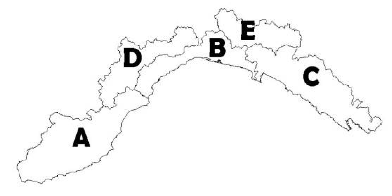
Table 11. The first row includes results for analysis 1, for comparison; the second row shows results considering events with damage or any other criticality; the third row considers the 62 cross-sections included in the A area and the events which had impacts, at least, on the A area; similarly, for B and C warning areas. D and E warning areas were excluded due to the very limited activation sample size available for them (23 and 32), for which the scores cannot be considered as reliable as for the other areas. A comparison is though possible between A, B, ad C areas, for which we wanted to check for any bias with respect to the overall results, e.g., if an area was characterized by a sensibly higher false or missed alarm rate or shorter warning times.
Considering the selection of critical events over the whole region, the sample is reduced by about 30% only, coherently with the fact that we observed the most activations during those events, but results did not substantially change from those in analysis 1. As expected, there was an increase in correct threshold 1 and 2 exceedances, i.e., +4% and 3%, respectively, but in favour of a decrease in correct non-exceedances, while the false and missed alarm rates remain practically unchanged. This may be due to the fact that many events had consequences on medium-large basins only, typically at the occurrence of non-convective meteorological events, characterised by higher cumulated rainfall values rather than intensities, or that these damages occurred in areas where no cross-sections are modelled in this chain or that criticalities were related to landslides and similar phenomena. Therefore, a more detailed analysis including information regarding observed criticalities is reported in Section 3.
As for the three warning areas considered, the A area showed a worse performance in terms of missed alarms, for both thresholds. FAR1 values are comparable. Overall, B and C area basins had comparable scores, with the higher rate of correct forecasts, both good as for threshold 2, and both good to very good FAR2 and MAR2, around 10% or less. These results may provide directions for further investigations about PhaSt performances for these particular events or maybe the cross-section thresholds; the latter aspect is better analysed in Section 3.
The statistics related to the warning times follow, including, again for comparison, results from analysis 1 (Table 12).
As for the warning times, results for the A and C areas are more similar and slightly better than in the B area. Mean Tw1 and 75th percentiles in the B area are about 5 to 10 min lower than in A, for instance. The frequency of higher anticipation times on threshold 2 exceedances is higher for A and C, where the 50th, and the 75th percentile in C, increases by 10 min; this might seem little for larger basins but it can acquire more relevance in the smallest drainage areas and be somehow useful during the operational phases.

3.3. Analysis 3: Modelling Performance Related to Observed Criticalities at the Basins Scale

As mentioned, the preparatory work for the latter analysis concerned the verification of the criticalities which occurred in the region, this time at the basin scale. As part of its activities, when a relevant hydrometeorological event occurs, ARPAL publishes a Hydrometeorological Event Report (REM). As a first step, based on such reports, the events causing severe ground effects or any other criticalities were selected. Then, the availability of the relative simulations in the archive was checked and, based on the available official information sources, namely the Civil Protection archives, the largest possible number of basins were listed, in which these criticalities were found. Comparing model results with observed impacts implies that here it is not sufficient to look at threshold forecast exceedances, but at basins activations, too: e.g., when the damage occurred in a drainage area whose corresponding cross-section did not activate at all, this implies a missed alarm. Unfortunately, the limited availability of information further reduced the sample; indeed, in order not to alter the results, in particular the percentage of correct non-activations and false alarms (the cases of observed zero criticality tend to be more numerous, at least apparently), the events with little information available had to be excluded. In addition, events which, despite having caused criticalities on medium-large basins, had no consequences on small basins were also excluded; the same was done when the damage reported was extremely localized or for which it was impossible to identify the basins, or, even if the basin was present in the damage file, it bore insufficient information. The result was a dataset of 25 events.
If the observed criticality flag was 0 (see Section 2), the modelling was considered correct in cases where: there was no activation; there was activation only; the basin activated with forecast threshold 1 exceedance, as these cases do not imply the occurrence of a criticality; on the other hand, a forecast threshold 2 exceedance was considered a false alarm.
If the observed criticality flag was equal to 1:
  • if there was no activation, the case is considered as a missed alarm;
  • if the basin activated, the case is considered as an underestimation, rather than a full missed alarm, since the model provided somehow a signal on that basin, even if not sufficiently clear; at the operational level, however, that signal can cause those who monitor in SOR to follow the situation with greater attention and proceed with further evaluations;
  • if the basin activated with forecast threshold 1 (only threshold 1) exceedance, we can consider this case can be considered a less serious underestimation than in the case of activation alone;
  • if threshold 2 is exceeded, that is correct modelling.
It is necessary to focus on the case of multiple activations during the same event, too. For a given basin and event, for example, the following case could occur: during a hydrometeorological event, damage occurs in a drainage area; the corresponding cross-section had activated twice, the first time without alarm threshold exceedance, the second time with exceedance. While the exceedance has to be correct, we cannot say anything about the first outcome, since we do not know the time at which the damage occurred and we would have to store information about the exact forecast time (Table 13). Looking for such additional information would be inefficient, besides these cases occurred with very low frequency. Therefore, they were excluded, without substantially affecting the activation sample size.
This is not an issue in the case of null observed criticality, as the flag is taken as a reference for all activations. The total sample size used to compute the scores is summarised in Table 14. This is even higher than the one used in Section 3.2, since, previously, activations only were considered.
Based on the previous considerations, the contingency tables had a slightly more complex structure as in Table 15, which reports the scores resulting from the model forecast.
Table 16 sums up all correct forecasts and all underestimations from the previous Table 15.
By summing up all correct predictions (84.2%) and totally wrong ones (missed and false alarms, 10.7%), promising scores are obtained.
The analysis was repeated, this time considering the observed discharge, too (i.e., simulated with observed rainfall field), to measure how much the modelling chain as a whole can detect criticalities, since, even while these are occurring, it is possible, although with a delay, to intervene and activate the rescue chain. To more easily visualise at a glance how these scores changed in comparison with the ones derived by analysing the forecast discharge scenarios only, the scores which, with respect to Table 15, have improved or worsened, are highlighted in green or red, respectively (Table 17). In Table 18 is possible to see a compact representation of results of Table 17.
As expected, the underestimation rate decreased in favour of an increase in minor underestimations and criticality detection rate, with the contribution of observed discharges; on the other hand, false alarms also increase, accompanied by a decrease in correct activations. The latter can be explained on one hand by the need to intervene on the thresholds; on the other hand, it must be accounted for that there are necessarily limits in the analysis of criticalities at the basin scale, due to the limited information availability: while, when damage is found, the criticality flag 1 is assigned with certainty, the null flag is always doubt.
By summing up all correct predictions (83.8%) and totally wrong ones (missed and false alarms, 12.7%), similar scores are obtained.
Afterwards, the scores conditionally on the occurrence, or not, of any criticality or damage were computed. Sättele et al. [18] estimate the reliability of a warning system for a debris flow alarm system by firstly computing the probability of detection, POD, and the probability of false alarms, PFA, given that a hazard event occurs or not. They estimate POD as the expected value of the ratio between the number of detected events by the number of total events and PFA as the expected value of the number of days with false alarms by the number of event-free days. Here, we are considering a (limited) set of hydrometeorological events, each one of them recording the occurrence, or not, of any criticality for each basin. Events with criticalities were therefore isolated to compute the scores conditionally on the occurrence of any criticality or damage, to further investigate correct criticality detections in relation to missed alarms, given that criticality occurs; similarly, the probability of false alarm, given that any criticality does not occur, was then estimated considering criticality-free events only. Criticality detection means alarm threshold exceedance. If we define POD and PFA based on these criteria, we obtain:
P O D = n u m b e r   o f   d e t e c t e d   c r i t i c a l i t i e s n u m b e r   o f   c r i t i c a l i t i e s ,
P F A = n u m b e r   o f   f a l s e   n o w c a s t   c r i t i c a l i t i e s n u m b e r   o f   c r i t i c a l i t y   f r e e   s i m u l a t i o n s .
Please note that by this definition of POD we do not refer to the number of total rainfall events, but to the number of observed criticalities and impacts on the territory, only; similarly, when defining PFA, we do not refer to the number of rainfall event-free days, but, out of these events, to which ones resulted in null criticalities, for specific basins. The resulting probability is not then a false alarm probability, e.g., per year, but per event, or, practically, per model simulation. This choice derives from the model nature and structure, too: as mentioned above (Section 2), the model chain is a monitoring chain, which does not run continuously, but at the occurrence of significant precipitation events, only. Therefore, exploiting the previously made classification in hit cases (correct threshold 2 exceedances), neutral cases (correct non-exceedances), false and missed alarms and by isolating the criticalities occurrences, [4], we obtain the scores as in Table 19. The first row is derived by considering nowcast scenarios, only; the second row accounts for both discharge nowcast and simulation with observed rainfall field.
The missed alarm rate cannot change, since derives from non-activation, therefore no observed or nowcast discharge is available.
By applying the second method, the activations without any exceedance decrease by more than 10%, as mentioned above, in favour of a slight increase in the minor underestimations, which only apparently did not point an improvement out, and an increase by about 10% in the correct detections, which reach up to about 50%.
Now, one could consider these outcomes from a more operative point of view. When a severe event occurs, characterized by very intense rainfall intensities, any cross-section activation leads the operator to focus on the area. Then, he/she does not interpret model results in an aseptic manner but proceeds with further evaluations. For instance, when an intense storm cell rapidly moves over an area so that alarm discharge flow is being nowcast at a specific cross-section, over which the most intense part of the cell is predicted to be localised, then the neighbouring cross-sections, which might not yet predict a threshold 2, or 1, exceedance will be kept under close observation, too. Therefore, we can try and sum up the correct detections with the minor underestimations, reaching up to 65% and any kind of signal, including activations only, reaching up to 82%. This means that, even with some delay and underestimations, the model chain provides a signal for more than 80% of the cases, which can be considered a good score.
The analogous table for PFA was not reported, since results did not substantially change with respect to Table 17: an overall PFA estimate of about 10% was obtained.
Besides the above considerations, it should be emphasized that analysis 3 is limited by the availability of information. Furthermore, in general, many false alarms may result from the impossibility of verifying that a criticality had occurred in the area or the choice of some too conservative thresholds; that is, it could be later investigated whether there are cases of exceeding the threshold both in the observation and in the forecast but the damage is null and verify this aspect.
Finally, similarly to Section 3.1, after estimating the overall scores we can have a look more in detail at the scores for each, this time not event, but basin. This choice is made, of course, because criticalities are evaluated at the basin scale and they can be correlated with the threshold values estimations. Table 20 summarises the scores computed for the 219 basins and can be read as follows: considering the last row, 52% of the basins had very good PFA, so between 0 and 10%; 31% of the basins had good PFA, so between 10 and 20%; and so on.
It is very important to highlight that we computed PFA as the ratio between the number of false exceedances during hydrometeorological events with no damage and the number of total hydrometeorological events in the region, not the total number of days with no event at all. In other words., the total number of hydrometeorological events with no damage on a basin was used, and not the total number of days with no damage on that basin. This is why the PFA may apparently seem too high.
Even though such values are not highly reliable due to the limited sample available for each basin, they allow us to assign a priority for a deeper further analysis. For instance, one could focus on the basins which provided the poorest scores in terms of false and missed alarm and investigate whether the discharge thresholds need to be modified, for instance with the support of up-to-date site-specific hydraulic studies.

4. Discussion

In order to estimate the reliability of SBMC, three different analyses were performed. The first analysis evaluated the performance of the model chain comparing forecast and observed discharge, from a purely modelling point of view; the second analysis employed a similar method, though applied at the warning area scale and considering critical events. The last analysis included a comparison of the modelling results with the criticalities observed at the basin scale, where information was available. Criteria were a priori established to define the goodness of results in terms of correct forecast, false, missed alarm rates (CFR, FAR, MAR) and anticipation times (Tw) on thresholds exceedances.
By observed discharge, it is here meant the simulated discharge using the observed rainfall field as input, hence the first analysis is more related to the PhaSt component performance rather than to the chain as a whole since the only varying forcing here is precipitation. The performance of the PhaSt algorithm itself has already been investigated in the past, for instance, comparing SBMC output employing different forcing by using observed rainfall data only, persistence forecast (assuming a rainfall pattern after the current time identical to the one occurred during the last hour) and, as the operative chain is currently working, by coupling observed rainfall data with the PhaSt nowcast scenarios. Thanks to radar rainfall field estimates, which PhaSt needs as input, significant improvements in the nowcast were observed [2]. Here, results were promising, too. The overall CFR related to the alarm (CFR2) has more than 80%, classified as good, FAR2 and MAR2 around 10% and 5% (good and very good), respectively. Computing such scores for each of the 99 events available, 72 events and 67 events had very good MAR2 and FAR2 (less than 10%), respectively, while 86 events had satisfactory up to very good CFR2. As for the warning times available prior to thresholds exceedances, they had a left-skewed distribution, which was expected given the very low dimensions of the basins and their sensitivity to intense, rapidly evolving, storm phenomena. Nevertheless, it is sometimes possible to have enough anticipation on the exceedances, particularly, on threshold 2. The event-averaged mean value of the warning time for threshold 2 (Tw2e) is estimated at around 15 min; the absolute mean value of Tw2 from the original dataset is around 20 min, but in some cases can exceed 1 h, or more depending on the event dynamics.
The second analysis focuses on events that had criticalities of any entity, at the warning area scale. Due to the very limited sample size of basins in D and E warning areas, recently added to the model chain, a comparison was only possible for the three coastal areas, A, B, C. This revealed, overall, better performances for basins in B and C as for nowcast threshold exceedances (good CRF2, around 10% higher than in A, where this was still satisfactory) and slightly better performances for A and C in terms of expected warning times, between 20 and 30 min.
Finally, the third analysis accounts for both activations and non-activations and employs a more articulated contingency table structure: in case of observed criticalities, non-activations only are considered as a completely missed alarm, while activations and threshold 1 exceedance, only, providing somehow a signal at a cross-section, are considered as detection with underestimation and light underestimation, respectively; a threshold 2 nowcast exceedance is then a full criticality detection. It is very complex to determine the exact trajectory and dynamics of intense and localized storm cells. Even when threshold 2 is not exceeded at a considered cross-section but this happens in neighbouring basins, all signals provided by the chain, e.g., threshold 1 exceedance only or just activation, could be accounted for, adopting a more risk-averse approach. The overall probability of detection of the model chain, given that a criticality occurs and considering all signals provided, is around 80%.
Similarly, the false alarm probability, given that a criticality does not occur, during a hydrometeorological event (not per day), is around 10%. The same scores were computed at the basin scale. Even if uncertain due to the limited sample available for each basin, they allow us to focus on basins that had the poorest performance and investigating the reasons why this happened; this may lead for instance to threshold values update.
Ideally, one aims at reducing the forecast uncertainties to obtain a correct forecast rate as close as possible to 100% and to issue a flood warning early enough or take timely measures in-event. Unfortunately, uncertainties cannot be reduced to zero and it is not always possible to timely forecast flash floods [6]. Particularly for very small basins (drainage area lower than 15 km2), small errors in the nowcast rainfall field can propagate through the model chain and strongly affect the nowcast discharge [9]. Nevertheless, useful tools can be developed to help to fill a gap as for the discharge forecasts in small and very small basins, for which information is usually hard to retrieve and for which the basins response times are very short, thanks to the availability of radar data, characterized by high spatial and temporal resolution. While natural variability has a stochastic nature, all types of uncertainty associated with imperfect knowledge or measurement errors are defined as epistemic or knowledge uncertainties; they are easier to detect and quantify and it should be possible to reduce them by further knowledge (e.g., by gathering additional data) [19]. Threshold values can be included in this type of uncertainty and may deserve further investigation and, possibly, updating.

5. Conclusions

The Small Basin Model Chain is a radar-based flood nowcasting chain employed in the Liguria region for event monitoring in basins with drainage areas lower than 15 km2, numerous in the region. A monitoring tool in such small basins is fundamental since they can potentially be dangerous for the population, especially in heavily urbanised areas [2]. This nowcasting chain was implemented over several years and consolidated during previous works, so that is now used for operative purposes. In particular, the performance of the PhaSt algorithm component has already been investigated in previous studies, showing significant nowcast improvements [2]. The nowcasting chain counts now more than 200 modelled cross-sections in the region, to have a capillary insight on what the impacts on the region are, driven by the meteorological events. This work was aimed at analysing model chain performances, finding the extent to which they can improve the predictability of flash floods for this particular kind of basins and improving the anticipation times. Overall, the correct forecast, false alarm and missed alarm rates, based on both model outcomes and the observed impacts or damages in the region, were considered satisfactory. Improving the anticipation time of flash flood events in such small basins is difficult, but during the monitoring phases, while the whole Civil Protection System is already alerted and ready to activate, having information even a few tens of minutes in advance can be helpful to take measures at specific sites.

Author Contributions

Conceptualization, M.R., F.M., F.S., F.G. and N.R.; methodology, M.R., F.M., F.S., F.G. and N.R.; software, M.R., F.M. and F.S.; validation, M.R. and F.M.; formal analysis, M.R. and F.M.; writing—original draft preparation, M.R. and F.M.; writing—review and editing, M.R., F.M., F.S. and F.G. All authors have read and agreed to the published version of the manuscript.

Funding

This research received no external funding.

Institutional Review Board Statement

Not applicable.

Informed Consent Statement

Not applicable.

Data Availability Statement

Data available on request. The data presented in this study are available on request from the corresponding author.

Conflicts of Interest

Authors declare no conflict of interest.

References

  1. Silvestro, F.; Gabellani, S.; Giannoni, F.; Parodi, A.; Rebora, N.; Rudari, R.; Siccardi, F. A hydrological analysis of the 4 November 2011 event in Genoa. Nat. Hazards Earth Syst. Sci. 2012, 12, 2743–2752. [Google Scholar] [CrossRef]
  2. Cummings, G.R. Flood Scenarios and Rainfall Nowcasting: Towards Building a Reliable Flood Nowcasting Procedure For Small and Very Small Basins. Ph.D. Thesis, Università degli Studi di Genova, Genova, Italy, April 2015. [Google Scholar]
  3. Straub, D. Landslide Risk Management and Assessment: Risk Mitigation and Management; Lecture Notes; Engineering Risk Analysis Group, Technical University of Munich: Munich, Germany, 2016. [Google Scholar]
  4. Sättele, M.; Bründl, M.; Straub, D. Quantifying the effectiveness of early warning systems for natural hazards. Nat. Hazards Earth Syst. Sci. 2016, 16, 149–166. [Google Scholar] [CrossRef] [Green Version]
  5. Corral, C.; Berenguer, M.; Sempere-Torres, D.; Poletti, L.; Silvestro, F.; Rebora, N. Comparison of two early warning systems for regional flash flood hazard forecasting. J. Hydrol. 2019, 572, 603–619. [Google Scholar] [CrossRef] [Green Version]
  6. Silvestro, F.; Rebora, N.; Cummings, G.; Ferraris, L. Experiences of dealing with flash floods using an ensemble hydrological nowcasting chain: Implications of communication, accessibility and distribution of the results. J. Flood Risk Manag. 2017, 10, 446–462. [Google Scholar] [CrossRef] [Green Version]
  7. Bales, J.D.; Wagner, C.R. Sources of uncertainty in flood inundation maps. J. Flood Risk Manag. 2009, 2, 139–147. [Google Scholar] [CrossRef]
  8. Milly, P.C.D.; Betancourt, J.; Falkenmark, M.; Hirsch, R.M.; Kundzewicz, Z.W.; Lettenmaier, D.P.; Stouffer, R.J. Stationarity is dead: Whither water management? Science 2008, 319, 573–574. [Google Scholar] [CrossRef] [PubMed]
  9. Silvestro, F.; Rebora, N. Operational verification of a framework for the probabilistic nowcasting of river discharge in small and medium size basins. Nat. Hazards Syst. Sci. 2012, 12, 763–776. [Google Scholar] [CrossRef] [Green Version]
  10. Metta, S.; Von Hardenberg, J.; Ferraris, L.; Rebora, N.; Provenzale, A. Precipitation Nowcasting by a Spectral-Based Nonlinear Stochastic Model. J. Hydrometeorol. 2009, 10, 1285–1297. [Google Scholar] [CrossRef]
  11. Nash, J.E. The Form of the Instantaneous Unit Hydrograph. Publ. IAHS 1957, 45, 114–121. [Google Scholar]
  12. Boni, G.; Ferraris, L.; Giannoni, F.; Roth, G.; Rudari, R. Flood probability analysis for an un-gauged watersheds by means of a simple distributed hydrologic model. Adv. Water Resour. 2007, 30, 2135–2144. [Google Scholar] [CrossRef]
  13. World Meteorological Organization. Discharge ratings using simple stage-discharge relation. In Manual on Stream Gauging, Computation of Discharge, 2nd ed.; World Meteorological Organization: Geneva, Switzerland, 2010; Volume 2, p. II.1-1. ISBN 978-92-63-11044-2. [Google Scholar]
  14. Beven, K. Rainfall-Runoff Modelling: The Primer, 2nd ed.; Wiley-Blackwell: Chichester, UK, 2012; ISBN 978-0-470-71459-1. [Google Scholar]
  15. Ramírez, J.A. Prediction and Modeling of Flood Hydrology and Hydraulics. In Inland Flood Hazards: Human, Riparian and Aquatic Communitie; Wohl, E., Ed.; Cambridge University Press: Cambridge, UK, 2000; ISBN 9780521189668. [Google Scholar]
  16. Gonzalo Rivera, H.; González Marentes, H.; Martínez Sarmiento, Ó.; Domínguez Calle, E.; Romero Pinzón, H.; Fajardo Sierra, M.; Zamudio Huertas, E.; González Hernández, Y.; Carvajal Contreras, M. Protocolo Para la Emisión de Los Pronósticos Hidrológicos (Translated Title: Protocol for the Issuance of Hydrological Forecasts); IDEAM; Imprenta Nacional de Colombia: Bogotá, Colombia, 2008; p. 106. ISBN 9789588067193. [Google Scholar]
  17. Moriasi, D.N.; Arnold, J.G.; Van Liew, M.W.; Bingner, R.L.; Harmel, R.D.; Veith, T.L. Model evaluation guidelines for systematic quantification of accuracy in watershed simulations. Am. Soc. Agric. Biol. Eng. 2007, 50, 885–900. [Google Scholar]
  18. Sättele, M.; Bründl, M.; Straub, D. Reliability and Effectiveness of Warning Systems for Natural Hazards: Concepts and Application to Debris Flow Warning. Reliab. Eng. Syst. Saf. 2015, 142, 192–202. [Google Scholar] [CrossRef] [Green Version]
  19. Beven, K.; Hall, J. Applied Uncertainty Analysis for Flood Risk Management, 2nd ed.; Imperial College Press: London, UK; Lancaster University and University of Oxford: Oxford, UK, 2014; ISBN 978-1848162709. [Google Scholar]
Figure 1. Model chain structure.
Atmosphere 12 00783 g001
Figure 2. Location of the Liguria region (green area) in Italy; modelled cross-sections in SBMC (red dots) and relative drainage areas (yellow areas), ranging from 0.2 up to 15 km2.
Atmosphere 12 00783 g002
Figure 3. SBMC output graphs for the modelled cross-section of Rupinaro creek on 1 November 2014 at 18:50 UTC (a) and 19:50 UTC (b). The date and time format on the X-axis is: YYMMDDHHmm. At 18:50 UTC (a) all nowcast discharge scenarios exceed one or both thresholds (pre-alarm and alarm thresholds), but this has not been observed, yet; the cross-section icon will colour as the worst-case scenario (orange, for alarm threshold nowcast exceedance) and the operator can take measures. At 19:50 UTC (b), 1 h later, alarm threshold (orange line) exceedance is observed and discharge is expected to further increase.
Atmosphere 12 00783 g003
Figure 4. Flood warning areas for the Liguria region.
Atmosphere 12 00783 g004
Figure 5. Relative frequency of the warning times on threshold 1 and 2 exceedances, by discreet 10-min classes, except the highest class, incorporating all anticipation times from 2 h up (a). Boxplots for Tw1 and Tw2; the horizontal line represents the median, which coincides with the minimum and with the 1st quartile of the empirical distribution (b).
Atmosphere 12 00783 g005
Table 1. Observed colour-coded criticalities by warning area resulting from previous analyses by Martina, F. for 3 sample events. Date format of the event: YYYYMMDD.
EventColour-Coded Criticality by Warning Area
ABCDE
20141104OrangeYellowOrangeYellowYellow
20141110RedRedRedOrangeYellow
20141115RedNAOrangeNARed
Table 2. Number of events used in the analyses, classified based on related criticalities or damages.
TotalDamageDamage A AreaDamage B AreaDamage C AreaDamage D AreaDamage E AreaDamage Single Basin
994818333310525
Table 3. Sample record for each basin activation, containing information used to compute the model chain scores. Q1 stands for threshold 1 discharge value, Q2 for threshold 2 discharge value. Subscripts “obs” and “frc” state observed and forecast discharge, respectively. Tw means the anticipation or warning time on threshold exceedances.
Activation n°Qobs ≥ Q1Qobs ≥ Q2Qfrc ≥ Q1Qfrc ≥ Q2Tw1 [min]Tw2 [min]
n0/10/10/10/1t1t2
Table 4. A priori criteria to define the goodness of the results. MAR, FAR, CFR stand for missed alarm, false alarm and correct forecast rates; Tw stands for warning time.
Performance RatingMAR [%]FAR [%]CFR [%]Tw [min]
Very good0 ≤ MAR < 100 ≤ FAR < 1090 < CFR ≤ 100>60
Good10 ≤ MAR < 2010 ≤ FAR < 2080 < CFR ≤ 9040–60
Satisfactory20 ≤ MAR < 3020 ≤ FAR < 3070 < CFR ≤ 8030
Sufficient30 ≤ MAR < 4030 ≤ FAR < 4060 < CFR ≤ 7020
Poor40 ≤ MAR < 5040 ≤ FAR < 5050 < CFR ≤ 6010
Very poorMAR ≥ 50FAR ≥ 50CFR ≤ 500
Table 5. Contingency table structure used for analyses 1 and 2.
Forecast Threshold ExceedanceObserved Threshold Exceedance
01
0Correct forecastMissed alarm
1False alarmCorrect forecast
Table 6. Sample used and total correct forecasts by threshold (analysis 1).
EventsBasins NumberActivations NumberCorrect Forecasts, Thr1Correct Forecasts, Thr2
99219442965.2%82.1%
Table 7. Contingency tables of pre-alarm (Thr1) and alarm (Thr2) thresholds exceedances (analysis 1). Subscript frc stands for forecast, obs stands for observed.
(a)(b)
Thr1obs = 0Thr1obs = 1 Thr2obs = 0Thr2obs = 1
Thr1frc = 042.3%20.0%Thr2frc = 067.8%6.6%
Thr1frc = 114.9%22.9%Thr2frc = 111.4%14.2%
Table 8. Performance ratings of forecast threshold exceedances by event. Subscript “e” stands for “event”.
Forecast Threshold Exceedance by EventPerformance Rating
Very GoodGoodSatisfactorySufficientPoorVery Poor
CFRe1101217191922
MARe136211511610
FARe1432713826
CFRe2382721724
MARe272204201
FARe2611913402
Table 9. Available sample size to compute basin average and event average warning time for a given basin or event.
Sample n°Tw1baTw2baTw1eaTw2ea
mean941910
max3933158121
Table 10. Sample size and interquartile range of the warning times (original dataset, Tw1 and Tw2) and event-averaged warning times (derived dataset, Tw1ea and Tw2ea); Qu. stands for quartile.
Warning TimeSample Size1st Qu.MedianMean3rd Qu.
Tw11898002220
Tw2921002530
Tw1ea94091825
Tw2ea74051425
Table 11. Sample size (activations), correct forecast, missed alarm and false alarm rates for thresholds 1 and 2 exceedances for events related to observed criticalities in different areas.
AreaEvents ConsideredBasins NumberActivations NumberCFR1FAR1MAR1CFR2FAR2MAR2
Liguria99219442965%15%20%82%11%7%
Liguria48219318865%14%20%81%12%7%
A186263959%12%28%73%15%12%
B3393141168%12%20%84%9%7%
C334851565%16%20%83%13%4%
Table 12. Sample size and interquartile range of the warning times for the original dataset (all basins and events) and reduced datasets of critical events by area; Qu. stands for quartile.
Sample1st Qu.MedianMean3rd Qu.
Tw1
Liguria (all events)1898002220
Liguria1502002420
A918002730
B1118002220
C1151002430
Tw2
Liguria (all events)921002530
Liguria7890102840
A4910102735
B544002230
C6190103040
Table 13. Exclusion of the records returning occurred criticality and threshold 2 non-exceedance in the case of multiple activations with divergent outcomes.
Flag| (Event and Basin)Basin Activation n°Qfrc ValuesScore
01Qfrc < Q2Correct
2Qfrc ≥ Q2False alarm
11Qfrc < Q2Non-assessable
2Qfrc ≥ Q2Correct
Table 14. Sample used in analysis 3. Basins number refers to the overall time period; “cases” refers to both basin activations and non-activations.
AreaEvents ConsideredBasins NumberTotal Cases
Liguria252195413
Table 15. Contingency matrix on expected threshold exceedances in relation to observed criticalities.
Modelled CriticalityObserved Criticality
01
Non-activationCorrect 58.0%Missed alarm 2.1%
ActivationCorrect 14.9%Underestimation 3.6%
Thr1 exc.Correct 6.4%Minor underestimation 1.5%
Thr2 exc.False alarm 8.6%Correct 4.9%
Table 16. Compact representation of Table 15.
Modelled CriticalityObserved Criticality
01
Thr2 non-exc.Correct 79.3%Underestimations 7.2%
Thr2 exc.False alarm 8.6%Correct 4.9%
Table 17. Contingency matrix for both forecast and observed threshold exceedances in relation to the observed criticalities. Worsened scores respect to Table 15 are represented in red and improved scores are represented in green.
Modelled CriticalityObserved Criticality
01
Non-activationCorrect 58.0%Missed alarm 2.1%
ActivationCorrect 11.8%Underestimation 2.1%
Thr1 exc.Correct 7.8%Minor underestimation 1.7%
Thr2 exc.False alarm 10.3%Correct 6.2%
Table 18. Compact representation of Table 17. Worsened scores respect to Table 16 are represented in red and improved scores are represented in green.
Modelled CriticalityObserved Criticality
01
Thr2 non-exc.Correct 77.6%Underestimations 5.9%
Thr2 exc.False alarm 10.3%Correct 6.2%
Table 19. Conditional model chain scores on the occurrence of critical events in single basin analysis, considering first forecast scenarios only and then both forecast and observed discharge.
AnalysisMissed AlarmUnderestimationMinor UnderestimationCorrect Detection
Qfrc17.6%29.8%12.4%40.3%
Qfrc, Qobs17.6%17.4%14.0%51.0%
Table 20. Performance ratings of forecast threshold exceedances by event. Subscript “b” stands for “basin”; corr stands for correct, lue stands for light underestimation and ues for any kind of underestimation.
Performance Rating by Basin
Very GoodGoodSatisfactorySufficientPoorVery Poor
PODb (Qfrc)
Thr2 corr15.4%1.4%6.5%7.0%1.9%57.0%
Thr2 corr + lue33.2%1.4%10.7%9.8%1.9%38.3%
Thr2corr + ues53.7%2.3%14.0%8.4%0.9%15.9%
PODb (Qfrc + Qobs)
Thr2 corr22.5%1.5%6.9%7.4%2.0%59.8%
Thr2 corr + lue34.8%1.5%11.3%10.3%2.0%40.2%
Thr2corr + ues56.4%2.5%14.7%8.8%1.0%16.7%
PFAb (Qfrc)59.9%32.5%7.5%2.4%0.5%0.5%
PFAb (Qfrc + Qobs)51.9%30.7%14.2%1.9%0.9%0.5%
Publisher’s Note: MDPI stays neutral with regard to jurisdictional claims in published maps and institutional affiliations.

