
Field Study of Metal Oxide Semiconductor Gas Sensors in Temperature Cycled Operation for Selective VOC Monitoring in Indoor Air


Abstract
:1. Introduction
2. Materials and Methods
2.1. Experimental Setup
- Thermo desorption gas chromatography-mass spectrometry (TD-GC-MS, Markes International Ltd, Llantrisant, Wales, UK, Thermo Fisher Scientific Inc., Waltham, MA, USA), similar to ISO 16000-6. TENAX® tubes were sampled with room air for 10 min at 50 mL/min. This system was used to quantify toluene during the release tests. The TD-GC-MS was calibrated in the same way with known concentrations from the GMA (7 tubes with 50–500 ppb toluene). The calibration was done 3 days before the specific release test. LOQ is smaller than 50 ppb, and the uncertainty is estimated to be 20%, based on the gas cylinder and the sampling method;
- Peak Performer 1 (Peak Laboratories LLC, Mountain View, CA, USA), a gas chromatograph with a reducing compound photometer as detector (GC-RCP), allows selective quantification of hydrogen with a LOD of 10 ppb and a resolution of 10% of reading or LOD (whichever is higher). The Peak Performer 1 requires nitrogen or another inert carrier gas from a pressure cylinder and provides a time resolution of 3.6 min;
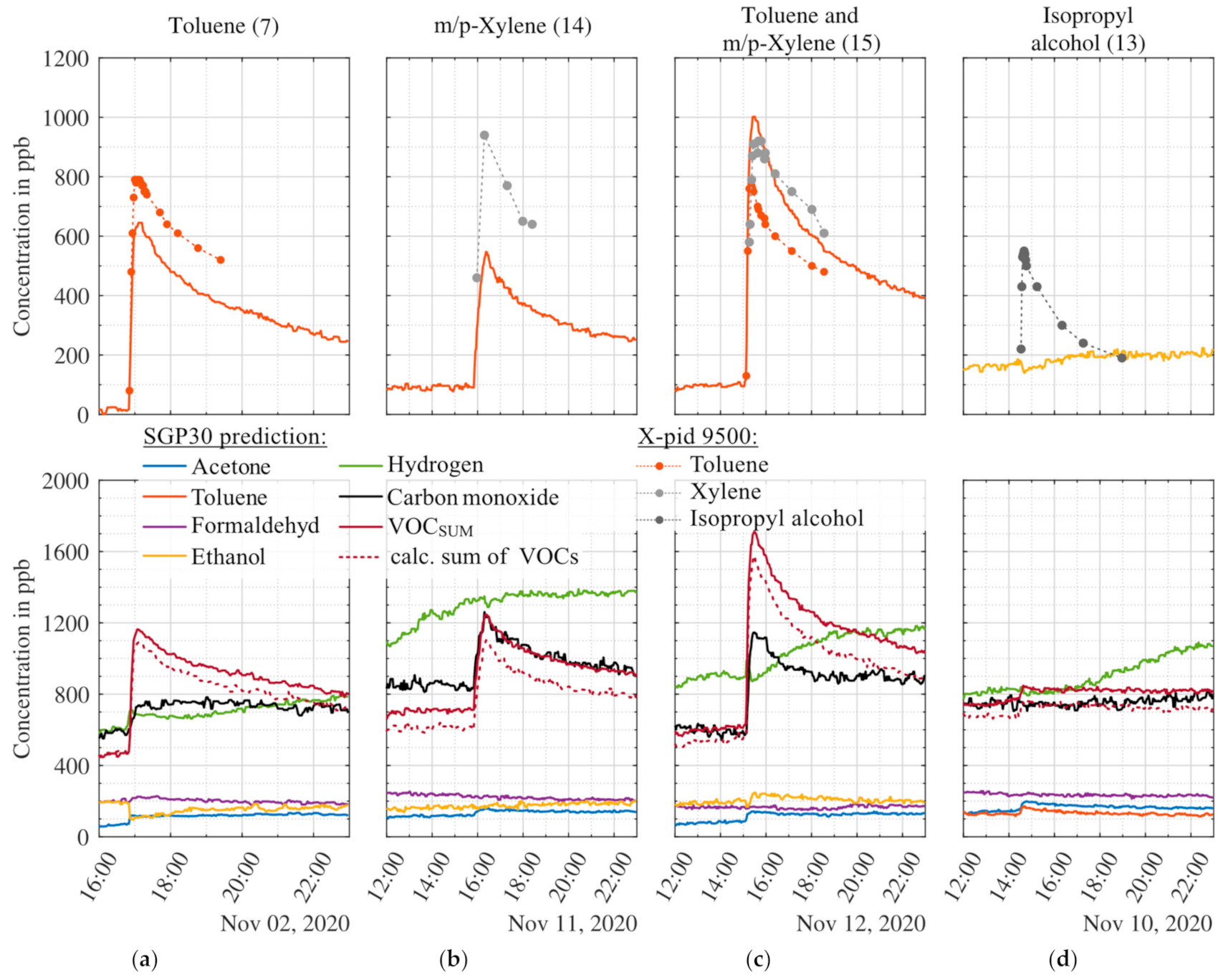
- Dräger X-pid 9500 (Dräger Safety AG & Co KGaA, Lübeck, Germany), a portable GC-PID offering a broad range of measured gases including acetone (LOQ: 500 ppb, LOD: 170 ppb), toluene (LOQ: 1000 ppb, LOD: 330 ppb), isopropyl alcohol (LOQ: 3000 ppb, LOD: 1000 ppb), and xylene (LOQ: 3000 ppb, LOD: 1000 ppb). The X-pid 9500 requires a daily function test with a test gas cylinder (10 ppm isobutene and 10 ppm toluene). Depending on the selected gases, a single measurement requires 2–3 min.
2.2. Calibration and Recalibration in the GMA
- Divide the list of VOCs found in studies in indoor environments into the most common chemical classes (also named substance types or groups): alcohols, aldehydes, alkanes, alkenes, aromatics, esters, glycols and glycol ethers, halocarbons, ketones, siloxanes, terpenes and organic acids;
- Sort the chemical classes according to their total concentrations;
- For each chemical class, select the substance with the highest concentration.
2.3. Field and Release Tests
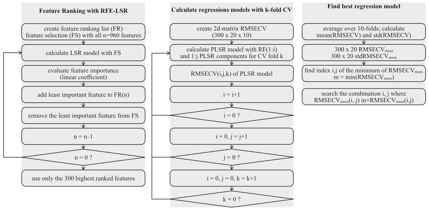
2.4. Data Evaluation
3. Results
3.1. Calibration and Recalibration
3.2. Field Tests
3.3. Uncalibrated Substances
4. Discussion
5. Conclusions
Author Contributions
Funding
Institutional Review Board Statement
Informed Consent Statement
Data Availability Statement
Acknowledgments
Conflicts of Interest
Appendix A


| Number | Time | Type of Event |
|---|---|---|
| 1 | 29 September, 09:35–09:48 | Door opened |
| 2 | 30 September, 09:24–09:58 | Window opened |
| 3 | 01 October, 09:10–09:30 | Window opened |
| 4 | 01 October, 11:47–12:05 | Door and window opened |
| 5 | 01 October, 18:30–02 October, 06:30 | No specifiable event |
| 6 | 2 October, 09:00–09:30 | Door and window opened |
| 7 | 02 October, 14:00–05 October, 10:00 | Days without events and human presence |
| 8 | 05 October, 10:10–10:30 | Door and window opened |
| 9 | 05 October and 05 October | Several short periods of human presence |
| 10 | 06 October, 13:08–16:51 | Door and window opened |
| 11 | 06 October, 17:42–18:44 | Release test: 1 ppm H2 |
| 12 | 07 October, 16:01–18:05 | Release test: 2 ppm H2 |
| 13 | 08 October, 10:46–11:00 | Door and window opened |
| 14 | 08 October to 13 October | Days without events and human presence |
| 15 | 13 October, 09:25–14:00 | Door and window opened, human presence |
| 16 | 13 October, 15:00 | Release test: toluene |
| 17 | 14 October, 09:30–10:05 | Door and window opened |
| 18 | 08 October to 13 October | Sporadic human presence, no specifiable events |
| 19 | 15 October, 09:00–09:30 | Door and window opened |
| 20 | 15 October, 15:00 | Release test: acetone |
| 21 | 16 October, 09:40–10:10 | Door and window opened |
| 22 | 16 October, 14:50 | Release test: acetone and toluene |
| 23 | 16 October, 18:00 | Release test: acetone and toluene |
| 24 | 17 October to 19 October | Days without events and human presence |
| 25 | 29 October, 12:55–13:10 | Door and window opened |
| 26 | 29 October to 02 November | Days without events and human presence |
| 27 | 02 November, 12:40–12:55 | Door and window opened |
| 28 | 02 November, 16:50 | Release test: toluene |
| 29 | 03 November, 10:55–11:10 | Door and window opened |
| 30 | 03 November, 15:30 | Release test: acetone followed by defect of the pump, human presence during fixing |
| 31 | 04 November, 09:00–09:15 | Door and window opened |
| 32 | 04 November, 16:22 | Release test: acetone |
| 33 | 05 November, 09:26–09:41 | Door and window opened |
| 34 | 05 November, 15:10 | Release test: acetone and toluene. Unidentified event due to construction inside the building |
| 35 | 05 November, 18:30–18:50 | Door and window opened |
| 36 | 06 November, 10:03 | Release test: limonene |
| 37 | 06 November to 09 November | Days without events and human presence |
| 38 | 09 November, 12:21–13:01 | Door and window opened |
| 39 | 09 November, 18:00 | Release test: ethanol |
| 40 | 10 November, 09:10–09:25 | Door and window opened |
| 41 | 10 November, 14:30 | Release test: isopropyl alcohol |
| 42 | 11 November, 09:28–09:48 | Door and window opened |
| 43 | 11 November, 15:49 | Release test: m/p-xylene |
| 44 | 12 November, 09:15–09:30 | Door and window opened |
| 45 | 12 November, 15:08 | Release test: toluene and m/p-xylene |
| 46 | 13 November, 09:28–11:06 | Door and window opened |
| 47 | 13 November, 14:30 | Release test: acetone, toluene, and ethanol |
| 48 | 13 November–16 November | Days without events and human presence |
| 49 | 16 November, 11:55–12:20 | Door and window opened |
| 50 | 16 November, 17:06–19:20 | Release test: 2 ppm H2 |
| 51 | 17 November, 09:54–10:24 | Door and window opened |
| 52 | 17 November, 18:24 | Release test: ethanol |
| 53 | 18 November, 09:36–09:56 | Door and window opened |
| 54 | 19 November, 12:02–16:02 | Release test: carbon monoxide (tea candle) |
References
- Asikainen, A.; Carrer, P.; Kephalopoulos, S.; Fernandes, E.D.O.; Wargocki, P.; Hänninen, O. Reducing burden of disease from residential indoor air exposures in Europe (HEALTHVENT project). Environ. Health 2016, 15, S35. [Google Scholar] [CrossRef] [PubMed]
- Settimo, G.; Manigrasso, M.; Avino, P. Indoor Air Quality: A Focus on the European Legislation and State-of-the-Art Research in Italy. Atmosphere 2020, 11, 370. [Google Scholar] [CrossRef] [Green Version]
- Spaul, W.A. Building-related factors to consider in indoor air quality evaluations. J. Allergy Clin. Immunol. 1994, 94, 385–389. [Google Scholar] [CrossRef] [PubMed]
- Herberger, S.; Herold, M.; Ulmer, H.; Burdack-Freitag, A.; Mayer, F. Detection of human effluents by a MOS gas sensor in correlation to VOC quantification by GC/MS. Build. Environ. 2010, 45, 2430–2439. [Google Scholar] [CrossRef]
- Buszewski, B.; Kesy, M.; Ligor, T.; Amann, A. Human exhaled air analytics: Biomarkers of diseases. Biomed. Chromatogr. 2007, 21, 553–566. [Google Scholar] [CrossRef]
- Veres, P.R.; Faber, P.; Drewnick, F.; Lelieveld, J.; Williams, J. Anthropogenic sources of VOC in a football stadium: Assessing human emissions in the atmosphere. Atmos. Env. 2013, 77, 1052–1059. [Google Scholar] [CrossRef]
- Pettenkofer, M. Über den Luftwechsel in Wohngebäuden; Literarisch-Artistische Anstalt der J.G. Cotta’schen Buchhandlung. 1858. Available online: https://opacplus.bsb-muenchen.de/title/BV013009721 (accessed on 17 May 2021).
- Liu, Y.; Misztal, P.K.; Xiong, J.; Tian, Y.; Arata, C.; Weber, R.J.; Nazaroff, W.W.; Goldstein, A.H. Characterizing sources and emissions of volatile organic compounds in a northern California residence using space- and time-resolved measurements. Indoor Air 2019, 29, 630–644. [Google Scholar] [CrossRef] [Green Version]
- Madou, M.J.; Morrison, S.R. Chemical Sensing with Solid State Devices; Academic Press, Inc.: San Diego, CA, USA, 1989; ISBN 978-0-12-464965-1. [Google Scholar]
- Bârsan, N.; Weimar, U. Understanding the fundamental principles of metal oxide based gas sensors; the example of CO sensing with SnO 2 sensors in the presence of humidity. J. Phys. Condens. Matter 2003, 15, 813–839. [Google Scholar] [CrossRef]
- Rüffer, D.; Hoehne, F.; Bühler, J. New digital metal-oxide (MOx) sensor platform. Sensors 2018, 18, 1052. [Google Scholar] [CrossRef] [Green Version]
- Schultealbert, C.; Baur, T.; Schütze, A.; Sauerwald, T. Facile Quantification and Identification Techniques for Reducing Gases over a Wide Concentration Range Using a MOS Sensor in Temperature-Cycled Operation. Sensors 2018, 18, 744. [Google Scholar] [CrossRef] [Green Version]
- Korotcenkov, G.; Cho, B.K. Instability of metal oxide-based conductometric gas sensors and approaches to stability improvement (short survey). Sens. Actuators B 2011, 156, 527–538. [Google Scholar] [CrossRef]
- ScioSense ENS160 Datasheet. Available online: https://www.sciosense.com/wp-content/uploads/documents/SC-001224-DS-1-ENS160-Datasheet-Rev-0.95.pdf (accessed on 4 April 2021).
- Schütze, A.; Baur, T.; Leidinger, M.; Reimringer, W.; Jung, R.; Conrad, T.; Sauerwald, T. Highly Sensitive and Selective VOC Sensor Systems Based on Semiconductor Gas Sensors: How to? Environments 2017, 4, 20. [Google Scholar] [CrossRef] [Green Version]
- Kohl, D.; Kelleter, J.; Petig, H. Detection of Fires by Gas Sensors. Sens. Updat. 2001, 9, 161–223. [Google Scholar] [CrossRef]
- Leidinger, M.; Sauerwald, T.; Reimringer, W.; Ventura, G.; Schütze, A. Selective detection of hazardous VOCs for indoor air quality applications using a virtual gas sensor array. J. Sens. Sens. Syst. 2014, 3, 253–263. [Google Scholar] [CrossRef] [Green Version]
- Bastuck, M.; Baur, T.; Richter, M.; Mull, B.; Schütze, A.; Sauerwald, T. Comparison of ppb-level gas measurements with a metal-oxide semiconductor gas sensor in two independent laboratories. Sens. Actuators B 2018, 273, 1037–1046. [Google Scholar] [CrossRef]
- Baur, T.; Schütze, A.; Sauerwald, T. Optimierung des temperaturzyklischen Betriebs von Halbleitergassensoren. Tech. Mess. 2015, 82, 187–195. [Google Scholar] [CrossRef]
- Schultealbert, C.; Baur, T.; Schütze, A.; Böttcher, S.; Sauerwald, T. A novel approach towards calibrated measurement of trace gases using metal oxide semiconductor sensors. Sens. Actuators B 2017, 239, 390–396. [Google Scholar] [CrossRef]
- Leidinger, M.; Schultealbert, C.; Neu, J.; Schütze, A.; Sauerwald, T. Characterization and calibration of gas sensor systems at ppb level–a versatile test gas generation system. Meas. Sci. Technol. 2018, 29, 015901. [Google Scholar] [CrossRef] [Green Version]
- Baur, T.; Bastuck, M.; Schultealbert, C.; Sauerwald, T.; Schütze, A. Random gas mixtures for efficient gas sensor calibration. J. Sens. Sens. Syst. 2020, 9, 411–424. [Google Scholar] [CrossRef]
- Hofmann, H.; Plieninger, P. Bereitstellung einer Datenbank zum Vorkommen von flüchtigen organischen Verbindungen in der Raumluft. WaBoLu Hefte 2008, 5, 161. [Google Scholar]
- Hofmann, H.; Erdmann, G.; Müller, A. Zielkonflikt energieeffiziente Bauweise und gute Raumluftqualität–Datenerhebung für flüchtige organische Verbindungen in der Innenraumluft von Wohn- und Bürogebäuden (Lösungswege); 2014. Available online: https://www.agoef.de/forschung/fue-ll-voc-datenerhebung/abschlussbericht.html (accessed on 17 May 2021).
- Traynor, G.W.; Apte, M.G.; Carruthers, A.R.; Dillworth, J.F.; Grimsrud, D.T.; Gundel, L.A. Indoor air pollution due to emissions from wood-burning stoves. Environ. Sci. Technol. 1987, 21, 691–697. [Google Scholar] [CrossRef] [PubMed] [Green Version]
- Schultealbert, C.; Amann, J.; Baur, T.; Schütze, A. Measuring Hydrogen in Indoor Air with a Selective Metal Oxide Semiconductor Sensor. Atmosphere 2021, 12, 366. [Google Scholar] [CrossRef]
- WHO. WHO Regional Office for Europe WHO Guidelines for Indoor Air Quality: Selected Pollutants; World Health Organization. Regional Office for Europe: Copenhagen, Denmark, 2010; Volume 9, ISBN 978-92-890-0213-4. [Google Scholar]
- Schultealbert, C.; Baur, T.; Schütze, A.; Sauerwald, T. Investigating the role of hydrogen in the calibration of MOS gas sensors for indoor air quality monitoring. In Proceedings of the Indoor Air, Philadelphia, PA, USA, 22–27 July 2018. [Google Scholar]
- Loh, W.-L. On Latin Hypercube Sampling. Ann. Stat. 1996, 24, 2058–2080. [Google Scholar] [CrossRef]
- Floor Plan of Building A5 1 at Saarland University. Available online: https://www.uni-saarland.de/fileadmin/upload/footer/grundriss/SBC-13_00-002.pdf (accessed on 4 April 2021).
- Bastuck, M.; Baur, T.; Schütze, A. DAV3E–a MATLAB toolbox for multivariate sensor data evaluation. J. Sens. Sens. Syst. 2018, 7, 489–506. [Google Scholar] [CrossRef] [Green Version]
- Youssef, S.; Zimmer, C.; Szielasko, K.; Schütze, A. Automatic feature extraction of periodic time signals using 3MA-X8 method. Tm Tech. Mess. 2019, 86, 267–277. [Google Scholar] [CrossRef]
- Bur, C.; Engel, M.; Horras, S.; Schütze, A. Drift compensation of virtual multisensor systems based on extended calibration, IMCS 2014-the 15th International Meeting on Chemical Sensors. In Proceedings of the IMCS 2014—The 15th International Meeting on Chemical Sensors, Buenos Aires, Argentina, 16–19 March 2014. [Google Scholar]
- Robin, Y.; Goodarzi, P.; Baur, T.; Schultealbert, C.; Schütze, A.; Schneider, T. Machine Learning based calibration time reduction for Gas Sensors in Temperature Cycled Operation. In Proceedings of the IEEE International Instrumentation and Measurement Technology Conference (I2MTC), Glasgow, Scotland, 17–20 May 2021. [Google Scholar]


| Chemical Class (Representative) | P90 in µg/m3 (ppb) | P95 in µg/m3 (ppb) |
|---|---|---|
| Alcohols (Ethanol) | 320 (~170) | 520 (~790) |
| Aldehydes (Formaldehyde) | 340 (~270) | 480 (~390) |
| Alkanes (n-Hexane, n-Heptane) | 180 (~50) | 350 (~90) |
| Aromatics (Toluene) | 190 (~50) | 370 (~90) |
| Esters (Ethyl acetate) | 140 (~30) | 280 (~70) |
| Ketones (Acetone) | 250 (~100) | 420 (~170) |
| Terpenes (Limonene, α-Pinene) | 170 (~30) | 330 (~60) |
| Organic acid (Acetic acid) | 150 (~60) | 240 (~100) |
| Substance | Min. | Max. |
|---|---|---|
| Carbon Monoxide | 150 ppb | 2000 ppb |
| Hydrogen | 400 ppb | 2000 ppb |
| Humidity | 25 %RH | 70 %RH |
| Acetone | 14 ppb | 300 ppb |
| Toluene | 4 ppb | 300 ppb |
| Formaldehyde | 1 ppb | 400 ppb |
| Ethanol | 4 ppb | 300 ppb |
| VOCsum | 300 ppb | 1200 ppb |
| Measurement Description | Unique Gas Mixtures | |
|---|---|---|
| Pre-tests | background with acetaldehyde instead of formaldehyde | 60 |
| background with acetaldehyde instead of formaldehyde and benzene instead of toluene | 15 | |
| Initial calibration | background only | 100 |
| background with modified acetone range: 14–1000 ppb | 100 | |
| background with modified toluene range: 4–1000 ppb | 100 | |
| background with modified ethanol range: 4–1000 ppb | 100 | |
| background with modified hydrogen range: 400–4000 ppb | 100 | |
| 1st field test period (4 weeks) | ||
| 1st Recalibration | background only | 100 |
| background with modified acetone range: 14–1000 ppb | 100 | |
| background with modified toluene range: 4–1000 ppb | 100 | |
| background with modified ethanol range: 4–1000 ppb | 100 | |
| background with modified hydrogen range: 400–4000 ppb | 100 | |
| 2nd field test period (3 weeks) | ||
| 2nd Recalibration | background only without toluene * | 100 |
| background only with m/p-xylene instead of toluene | 50 | |
| background only with limonene instead of toluene | 50 | |
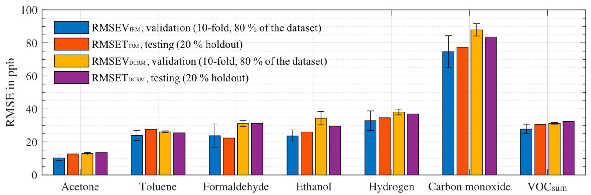
| Substance | RMSEDCRM in ppb | GMA Accuracy 1 in % (ppb) | GMA Precision 1 in % (ppb) |
|---|---|---|---|
| Acetone | 13.6 | 5.0–6.5 (1–50) | 0.7–4.1 (1–6) |
| Toluene | 25.5 | 2.1–2.8 (0.1–23) | 0.5–1.8 (0.1–10) |
| Formaldehyde | 31.3 | 20.0–20.3 (0.3–82) | 0.6–3.5 (0.1–10) |
| Ethanol | 29.6 | 3.1–4.7 (0.2–35) | 0.6–3.5 (0.2–17) |
| VOCsum | 32.5 | 1.8–15 (8–93) | 0.6–1.8 (2–19) |
| Carbon Monoxide | 83.6 | 2.2–4.2 (6–49) | 0.9–3.7 (6–20) |
| Hydrogen | 37.0 | 2.1–3.9 (16–85) | 0.5–3.3 (14–23) |
| Release | Event | Time | Substance (Type of Release) | Released Amount of Substance (Approx. Increase in Room Conc.) |
|---|---|---|---|---|
| Pre-tests and Initial calibration | ||||
| 1 | 11 | 06 October, 17:42 | Hydrogen (MFC, gas cylinder) | 2000 ppm @ 500 mL/min for 62 min (~1 ppm ± 4%) |
| 2 | 12 | 07 October, 16:01 | Hydrogen (MFC, gas cylinder) | 2000 ppm @ 500 mL/min for 124 min (~2 ppm ± 4%) |
| 3 | 16 | 13 October, 15:00 | Toluene (MFC, gas cylinder) | 100 ppm @ 500 mL/min for 497 min (~300 ppb ± 10%) |
| 5 | 22 | 16 October, 14:50 | Acetone (evaporation) Toluene (evaporation) | 0.114 mL (~600 ppb ± 10%) 0.164 mL (~600 ppb ± 10%) |
| 6 | 23 | 16 October, 18:00 | Acetone (evaporation) Toluene (evaporation) | 0.114 mL (~600 ppb ± 10%) 0.164 mL (~600 ppb ± 10%) |
| 1st Recalibration | ||||
| 7 | 28 | 02 November, 16:50 | Toluene (evaporation) | 0.164 mL (~600 ppb ± 10%) |
| 9 | 32 | 04 November, 16:22 | Acetone (evaporation) | 0.114 mL (~600 ppb ± 10%) |
| 10 | 34 | 05 November, 15:10 | Acetone (evaporation) Toluene (evaporation) | 0.114 mL (~600 ppb ± 10%) 0.164 mL (~600 ppb ± 10%) |
| 11 | 36 | 06 November, 10:03 | Limonene (evaporation) | 0.251 mL (~600 ppb ± 10%) |
| 12 | 39 | 09 November, 18:00 | Ethanol (evaporation) | 0.1 mL (~664 ± 10%) |
| 13 | 41 | 10 November, 14:30 | Isopropyl alcohol (evaporation) | 0.12 mL (~600 ppb ± 10%) |
| 14 | 43 | 11 November, 15:49 | m/p-Xylene (evaporation) | 0.189 mL (~600 ppb ± 10%) |
| 15 | 45 | 12 November, 15:08 | Toluene (evaporation) m/p-Xylene (evaporation) | 0.164 mL (~600 ppb ± 10%) 0.189 mL (~600 ppb ± 10%) |
| 16 | 47 | 13 November, 14:30 | Acetone (evaporation) Toluene (evaporation) Ethanol (evaporation) | 0.114 mL (~600 ppb ± 10%) 0.164 mL (~600 ppb ± 10%) 0.1 mL (~664 ppb ± 10%) |
| 17 | 50 | 16 November, 17:06 | Hydrogen (MFC, gas cylinder) | 2000 ppm @ 500 mL/min for 134 min (~2 ppm ± 4%) |
| 18 | 52 | 17 November, 18:24 | Ethanol (evaporation) | 0.1 mL (~664 ppb ± 10%) |
| 19 | 54 | 19 November, 12:02 | Carbon monoxide etc. (tea candle) | 4 h burn time |
| 2nd Recalibration |
Publisher’s Note: MDPI stays neutral with regard to jurisdictional claims in published maps and institutional affiliations. |
© 2021 by the authors. Licensee MDPI, Basel, Switzerland. This article is an open access article distributed under the terms and conditions of the Creative Commons Attribution (CC BY) license (https://creativecommons.org/licenses/by/4.0/).
Share and Cite
Baur, T.; Amann, J.; Schultealbert, C.; Schütze, A. Field Study of Metal Oxide Semiconductor Gas Sensors in Temperature Cycled Operation for Selective VOC Monitoring in Indoor Air. Atmosphere 2021, 12, 647. https://doi.org/10.3390/atmos12050647
Baur T, Amann J, Schultealbert C, Schütze A. Field Study of Metal Oxide Semiconductor Gas Sensors in Temperature Cycled Operation for Selective VOC Monitoring in Indoor Air. Atmosphere. 2021; 12(5):647. https://doi.org/10.3390/atmos12050647
Chicago/Turabian StyleBaur, Tobias, Johannes Amann, Caroline Schultealbert, and Andreas Schütze. 2021. "Field Study of Metal Oxide Semiconductor Gas Sensors in Temperature Cycled Operation for Selective VOC Monitoring in Indoor Air" Atmosphere 12, no. 5: 647. https://doi.org/10.3390/atmos12050647