Article

Method for Measuring the Second-Order Moment of Atmospheric Turbulence

1
School of Science, Jiujiang University, Jiujiang 332005, China
2
Information Engineering School, Nanchang University, Nanchang 330031, China
3
Key Laboratory of Atmospheric Optics, Anhui Institute of Optics and Fine Mechanics, Chinese Academy of Sciences, Hefei 230031, China
*
Author to whom correspondence should be addressed.
Atmosphere 2021, 12(5), 564; https://doi.org/10.3390/atmos12050564
Submission received: 27 March 2021 / Revised: 25 April 2021 / Accepted: 26 April 2021 / Published: 28 April 2021
(This article belongs to the Special Issue Structure of Atmospheric Turbulence)

Abstract

:
The turbulence moment of order m (μm) is defined as the refractive index structure constant Cn2 integrated over the whole path z with path-weighting function zm. Optical effects of atmospheric turbulence are directly related to turbulence moments. To evaluate the optical effects of atmospheric turbulence, it is necessary to measure the turbulence moment. It is well known that zero-order moments of turbulence (μ0) and five-thirds-order moments of turbulence (μ5/3), which correspond to the seeing and the isoplanatic angles, respectively, have been monitored as routine parameters in astronomical site testing. However, the direct measurement of second-order moments of turbulence (μ2) of the whole layer atmosphere has not been reported. Using a star as the light source, it has been found that μ2 can be measured through the covariance of the irradiance in two receiver apertures with suitable aperture size and aperture separation. Numerical results show that the theoretical error of this novel method is negligible in all the typical turbulence models. This method enabled us to monitor μ2 as a routine parameter in astronomical site testing, which is helpful to understand the characteristics of atmospheric turbulence better combined with μ0 and μ5/3.

1. Introduction

Random fluctuations of atmospheric refractive index, also called optical turbulence, severely influence the performance of optical systems that operate in or through the atmosphere, such as adaptive optics systems, interferometers, optical wireless communication systems, and laser radar systems [1,2,3]. These optical systems are often used in scientific fields including optical astronomy, the propagation of laser radiation through random media, and imaging through turbulence [1,2,3,4,5]. It is of great significance to evaluate the optical effects of turbulence in these optical systems.
In evaluating the optical effects of turbulence, it is convenient to define the turbulence moment of order m as:
μ m = 0 L C n 2 ( z ) z m d z ,
where Cn2 is the refractive index structure constant and z denotes the position along the path for propagation from z = L to a receiver at z = 0. Three turbulence moments most frequently used are:
  • Zero-order, m = 0, for evaluating the seeing r0;
  • Five-thirds-order, m = 5/3, for evaluating the isoplanatic angle θ0;
  • Second-order, m = 2, for evaluating overall tilt errors [1].
Tilt isoplanatic angle (θTA), also called isokinetic angle or isoplanatic angle for image motion, is directly related to the second-order moment of turbulence (μ2), which has a form for small angles (θ < D/40000) [1,3]:
θ T A = ( 0.668 k 2 μ 2 D 1 / 3 ) 1 / 2
where D is the aperture size of the receiver telescope and k is the wave number. Tilt isoplanatic angle determines the sky coverage in an adaptive optics system with a laser guide star [1,6], and it is a limiting factor in image stabilization and wide field imaging [7]. Other turbulence effects, such as the Zernike anisoplanatism of a collimated beam for small angles and scintillation with large apertures of a collimated beam, are also related to μ2 [3].
Optical effects of turbulence are directly related to turbulence moments. As such, it is necessary to measure turbulence moments. Indeed, the first two turbulence moments, μ0 and μ5/3, which correspond to r0 and θ0, respectively, have been monitored as routine parameters especially in astronomical site testing for a long time [8,9,10]. It is possible to compute μ2 from the restored turbulence profile obtained by turbulence profilers, such as MASS (Multi-Aperture Scintillation Sensor) [11], SLODAR (Slope Detection and Ranging) [12,13,14], PML (Profiler of Moon Limb) [15], etc. [16]; direct measurement of μ2 has not been reported.
We studied the theoretical feasibility of direct measurements of μ2 using a stellar source. Theoretical results for path-weighting function of the covariance of the irradiance are developed and a novel method for measuring μ2 using two receiver apertures and a stellar source is proposed.

2. Theoretical Basis

For convenience, u = z/L is defined as the normalized position along the path, and thus μ2 can be rewritten as:
μ 2 = L 3 0 1 C n 2 ( u L ) u 2 d u
The key problem for measuring μ2 is to make the measurable quantity have a normalized path-weighting function W0(u), which is approximately equal to u2:
W 0 ( u ) u 2
Assuming the Rytov approximation and Kolmogorov turbulence, using the analytic approach developed by Sasiela (2007), the log-amplitude covariance function on an aperture, CχA(d), can be written as:
C χ A ( d ) = 0.132 π 2 k 2 L 0 1 C n 2 ( u L ) W C ( u , d ) d u
where χA is the log-amplitude collected by an aperture, k is the wave number, d is the center-to-center distance of two receiver apertures, and WC(u,d) is the path-weighting function of CχA(d), which is given by Equation (6) (for convenience later, WC(u,d) is replaced with WC(u)):
W C ( u ) = 0 F ( γ κ ) κ 8 / 3 J 0 ( γ κ d ) sin 2 ( κ 2 γ u L 2 k ) d κ
Here, γ is the propagation parameter, which depends on the geometric divergence of the light wave and has the simple value γ = 1 for plane waves, and γ = 1 − z/L for spherical waves, κ is the spatial wavenumber transverse to the z direction, and F(γκ) is the filter function. The form of the filter function depends on the receiver aperture and has the form [3]:
F ( γ κ ) = [ 4 J 1 ( γ κ D / 2 ) / γ κ D ] 2
for a circular aperture with diameter D.
Filter functions considered in this paper are for circular apertures and plane waves, which are commonly encountered in astronomical observations. The Fresnel number is defined as FN = D2/λ0L, where λ0 is the effective wavelength that depends on the particular star chosen for observations [17,18]. Substituting Equation (7) into Equation (6) and replacing κD by κ results in:
W C ( u ) = D 5 3 0 κ 8 3 [ 2 J 1 ( κ / 2 ) κ / 2 ] 2 J 0 ( κ d D ) sin 2 ( κ 2 u 4 π F N ) d κ
We call WC(u)/Max(WC(u)) the normalized path-weighting function W0(u). From Equation (8), it can be seen that the shape of W0(u) depends on d/D and FN. It is well known that the normalized path-weighting function for stellar scintillation (i.e., normalized WC(u) for d = 0 and γ = 1) approximates to u2 for very large aperture [19]. However, it is costly and inconvenient to use a large aperture telescope. We attempted to find whether there is a desirable set of d/D and FN that makes W0(u) approximate to u2, while maintaining D sufficiently small for a compact device.

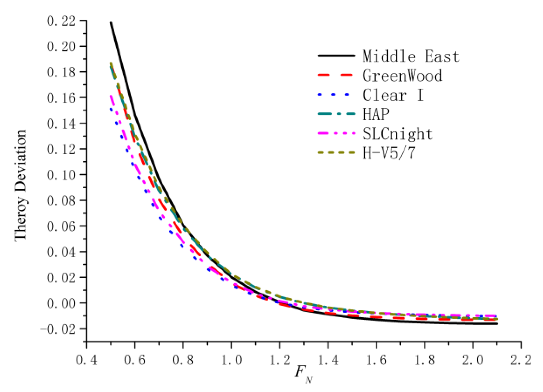
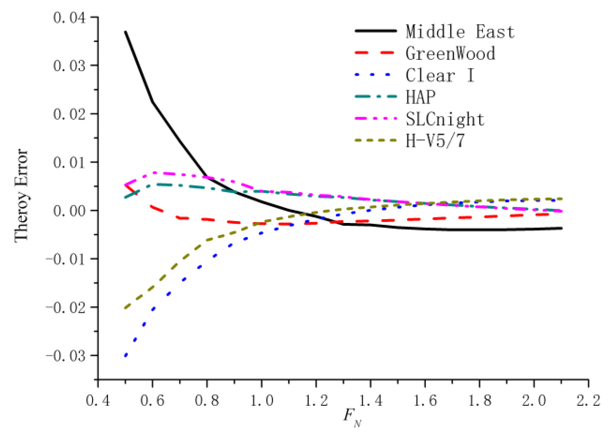
3. Numerical Results and Analysis

We used the root-mean-square error (RMSE) of W0(u) fitting to u2, ERMS to evaluate the fitting accuracy. ERMS is expressed as:
E R M S = i = 1 N ( W 0 ( u i ) u i 2 ) 2 N
where N is the number of equally divided paths. We set N = 1000. Through numerical analysis, we found that the path-weighting function of log-amplitude covariance for plane waves (i.e., W0(u) for γ = 1) can be approximated to u2 when FN > 0.5. When FN ∈ [1,2] the fitting accuracy is very high, and the corresponding best d/D has small range of variation between 0.57 and 0.5. The best d/D means that ERMS is the minimum when FN is fixed. Through numerical analysis, we also found the least RMSE, ERMS = 1.17 × 10⁻³, corresponding to the best set of d/D = 0.52 and FN = 1.595. This value is one order of magnitude smaller compared to the least RMSE of W0(u) (for d = 0, γ = 1) fitting to u5/3 [19]. The normalized path-weighting function of log-amplitude covariance for plane waves W0(u) with the best set of d/D and FN is plotted in Figure 1. Path-weighting function u2 and the normalized deviation (W0(u) − u2)/u2 are also given for comparison.
The overlap of the two path weighting functions in Figure 1 shows that the fitting accuracy is very high.
The best d/D in different FN and the corresponding ERMS are plotted in Figure 2. These numerical results are then used to design the instrument for measuring the second-order moment of turbulence μ2. Specifically, the aperture size D and separations d need to be optimized.
First, we need to determine the minimum turbulence layer height h0 over which turbulence path-weighting function should be fitted with high accuracy. The turbulence is usually assumed to be zero above 30 km [3]. Numerical calculations have also shown that the contribution of turbulence above 20 km to isoplanatic angle θ0 is negligible (less than 2% in typical turbulence models) [18].
Again (Figure 3), we can see that the contribution of the turbulence above 20 km is negligible and we set h0 to 20 km.
Secondly, we need to determine the range of D, the diameter of the apertures. As mentioned before, FN = D2/λ0L, and L = h0secϕ, where ϕ is the zenith angle and should be less than 45° to ensure the Rytov approximation [18]. In practice, d/D remains fixed but FN changes because ϕ is changing due to the movement of the observed star. As found from Figure 2, when FN ∈ [1,2], the fitting accuracy is very high (ERMS is less than 0.3%) and the corresponding range of d/D is constrained between 0.57 and 0.5. We take the approximate central value of 0.53, so the separation (center-to-center) of the aperture is d = 0.53D. This means that both the apertures overlap. Note that D = (FNλ0h0secϕ)1/2, FN ∈ [1,2], ϕ ∈ [0,45°]. If λ0 = 600nm, the range of D is roughly [11,18 cm].
Thirdly, we calculated the theoretical error introduced by this covariance method. The deviation of μ2 calculated by normalized covariance path-weighting function W0(u) instead of u2 when d/D = 0.53 is evaluated with different Fresnel numbers FN and various typical turbulence models. Specifically, these turbulence models are Hufnagel–Valley (H-V), SLCnight, Greenwood, CLEAR I [20], Hufnagel/Andrews/Phillips (HAP) [21], and Middle East [22]. These models are expressed as [20,21,22]:
C n 2 ( h ) = 5.94 × 10 23 ( W / 27 ) 2 h 10 e h + 2.7 × 10 16 e 2 h / 3 + A e 10 h , ( H-V )
C n 2 ( h ) = { 8.40 × 10 15   if   h 18.5   2.87 × 10 12 h 2   if   18.5   <   h 110 2.5 × 10 16   if   110 < h 1500 8.87 × 10 7 h 3   if   1500 < h 7200 2.00 × 10 16 h 0.5   if   7200 < h 20,000 0   otherwise ,   ( SLC-night )
C n 2 ( h ) = [ 2.2 × 10 13 ( h + 10 ) 13 + 4.7 × 10 17 ] e h 4000 ,   ( Greenwood )
C n 2 ( h ) = { 10 [ 10.7052 4.3507 h 1000 + 0.8141 ( h 1000 ) 2 ] ( if   1230 h 2130 ) 10 [ 16.2897 + 0.0335 h 1000 0.0134 ( h 1000 ) 2 ] ( if   2130 h 10,340 ) 10 [ 17.0577 0.0449 h 1000 0.0005 ( h 1000 ) 2 ]     10 [ 0.6181 e 0.5 ( h 1000 15.5617 3.4666 ) 2 ]     ( if   10,340 h 31,230 )     , ( CLEAR   I )    
C n 2 ( h ) = 2.7 × 10 16 e h 1500 + A ( 1 h + 1 ) 4 3 + 5.94 × 10 53 h 10 ( W 27 ) 2 e h 1000 ,     ( HAP )
C n 2 ( h ) = 8 × 10 14 e h 200 + 1 × 10 15 e h 1250 4.12 × 10 53 h 10 e h 1000 + 4.5 × 10 16 e ( h 2500 ) 2 2 100 2 + 1.6 × 10 16 e ( h 5300 ) 2 2 130 2 + 6.4 × 10 16 e ( h 8500 ) 2 2 130 2 + 5.5 × 10 17 e h 5700 ,   ( Middle   East )
where h is the altitude above ground, in meters, except for CLEAR I model in which h is the altitude above mean sea level. Curves of these turbulence models are shown in Figure 4 for reference.
The deviation of μ2, Dev, is given by:
D e v = 0 1 C n 2 ( u L ) W 0 ( u ) d u 0 1 C n 2 ( u L ) u 2 d u 0 1 C n 2 ( u L ) u 2 d u
As shown in Figure 5, it can be seen that Dev is dependent on FN, as expected. Dev is positive and decreases to zero as FN increases from 0.5 to 1.5, and the difference between the various models also decreases. This behavior is due to the increase in fitting accuracy as FN increases from 0.5 to about 1.5, as shown in Figure 2.
Even if it is not rigorous enough, Dev can be seen as an inherent offset; after the subtraction of the mean value, the absolute error becomes small. We take this absolute error as the theoretical error of the covariance method in those turbulence models, as shown in Figure 6.
From Figure 6, it can be seen that the theoretical error is negligible when FN ∈ [1,2] where fitting accuracy is very high, and it is less than 3.7% when FN ∈ [0.5,1], which is also acceptable. Therefore, we can extend the range of FN to [0.5,2], and then the range of D is roughly [8,18 cm]. It should be noted here that the fitting accuracy drops dramatically when FN decrease from 1 to 0.5. Although the theoretical error is acceptable, it is recommended to use the range FN ∈ [1,2].
Considering the compactness of the measurement system, we can select D from the range [8,12 cm], and d = 0.53D. Therefore, it is possible to construct the instrument for measuring μ2 by using a 160 mm or larger diameter telescope with a mask containing two apertures at required separations. These two apertures will overlap for d = 0.53D < D. To obtain irradiance variation on each aperture, two side areas of the receiver aperture that are not overlapped should be equipped with two thin-edge prisms (with opposite deflecting directions) to separate the spot images, as shown in Figure 7. Then, the light is split into three distinct beams, and the beams will focus into three separate spots, which can be received by three photomultipliers.

4. Conclusions

In conclusion, through numerical analysis, we found that the path-weighting function of log-amplitude covariance on two apertures with desired separation (d ≈ 0.53D) for plane waves approximates to the square of the path position when FN > 0.5. The theoretical error of the covariance method in typical turbulence models is negligible when FN ∈ [1,2] and less than 3.7% when FN ∈ [0.5,1]. This indicates that the second-order moment of turbulence μ2 can be measured through the covariance of irradiance emitted from a stellar source using two receiver apertures with desired separation and aperture diameter. It should be noted that this method is valid for Rytov numbers less than 0.35, because our approach was based on the Rytov approximation [3]. The theoretical error of the covariance method is negligible in typical turbulence models. This method should allow us to monitor μ2 of an integrated atmosphere in real time. This means that μ2 can also be monitored as a routine parameter such as μ0 and μ5/3 (corresponding to r0 and θ0, respectively) in site testing. The measured μ2 estimate is helpful to understand the characteristics of atmospheric turbulence in terms of integrated tip-tilt and isokinetic angle, providing complementary information to the seeing and isoplanatic angle provided by μ0 and μ5/3. In the future, experimental work will be conducted to validate this novel method for measuring μ2.

Author Contributions

Conceptualization, H.S. and L.Y.; methodology, H.S.; software, L.Y.; validation, H.S., L.Y. and X.J.; formal analysis, H.S.; investigation, L.Y.; data curation, F.T.; writing—original draft preparation, H.S.; writing—review and editing, H.S. and L.Y.; funding acquisition, H.S. and L.Y. All authors have read and agreed to the published version of the manuscript.

Funding

This research was funded by the National Natural Science Foundation of China, grant numbers 61665004 and 41605007.

Institutional Review Board Statement

Not applicable.

Informed Consent Statement

Not applicable.

Data Availability Statement

The data presented in this study are available on request from the corresponding author.

Acknowledgments

The authors would like to thank the Editor and the anonymous reviewers for their insightful comments and suggestions.

Conflicts of Interest

The authors declare no conflict of interest.

References

  1. Hardy, J.W. Adaptive Optics for Astronomical Telescopes; Oxford University Press: New York, NY, USA, 1998; pp. 98–268. [Google Scholar]
  2. Andrews, L.C.; Phillips, R.L. Laser Beam Propagation through Random Media; SPIE Press: Bellingham, WA, USA, 2005; pp. 14–32. [Google Scholar]
  3. Sasiela, R.J. Electromagnetic Wave Propagation in Turbulence: Evaluation and Application of Mellin Transforms; SPIE Press: Bellingham, WA, USA, 2007; pp. 69–88. [Google Scholar]
  4. Roggemann, M.C.; Welsh, B.M.; Hunt, B.R. Imaging through Turbulence; CRC Press: London, UK; New York, NY, USA, 2018. [Google Scholar]
  5. Tyson, R.K. Principles of Adaptive Optics, 4th ed.; CRC Press: London, UK; New York, NY, USA, 2016; pp. 37–54. [Google Scholar]
  6. Olivier, S.S.; Max, C.E.; Gavel, D.T.; Brase, J.M. Tip-Tilt Compensation: Resolution Limits for Ground-based Telescopes Using Laser Guide Star Adaptive Optics. Astrophys. J. 1993, 407, 428–439. [Google Scholar] [CrossRef]
  7. Kaiser, N.; Tonry, J.L.; Luppino, G.A. A new strategy for deep wide-field high-resolution optical imaging. Publ. Astron. Soc. Pac. 2000, 112, 768–800. [Google Scholar] [CrossRef] [Green Version]
  8. Sarazin, M.; Roddier, F. The ESO differential image motion monitor. Astron. Astrophys. 1990, 227, 294–300. [Google Scholar]
  9. Aristidi, E.; Agabi, A.; Fossat, E.; Azouit, M.; Martin, F.; Sadibekova, T.; Travouillon, T.; Vernin, J.; Ziad, A. Site testing in summer at Dome C., Antarctica. Astron. Astrophys. 2005, 444, 651–659. [Google Scholar] [CrossRef] [Green Version]
  10. Skidmore, W.; Els, S.; Travouillon, T.; Riddle, R.; Schöck, M.; Bustos, E.; Seguel, J.; Walker, D. Thirty Meter Telescope site testing V: Seeing and isoplanatic angle. Publ. Astron. Soc. Pac. 2009, 121, 1151–1166. [Google Scholar] [CrossRef]
  11. Kornilov, V.; Tokovinin, A.; Shatsky, N.; Voziakova, O.; Potanin, S.; Safonov, B. Combined MASS–DIMM instruments for atmospheric turbulence studies. Mon. Not. R. Astron. Soc. 2007, 382, 1268–1278. [Google Scholar] [CrossRef] [Green Version]
  12. Wilson, R.; Bate, J.; Guerra, J.C.; Hubin, N.; Sarazin, M.; Saunter, C. Development of a portable SLODAR turbulence profiler. Advancements in Adaptive Optics. In Proceedings of the SPIE Astronomical Telescopes and Instrumentation, Glasgow, UK, 25 October 2004. [Google Scholar] [CrossRef] [Green Version]
  13. Townson, M.J. Correlation Wavefront Sensing and Turbulence Profiling for Solar Adaptive Optics. Ph.D. Thesis, The University of Durham, Durham, UK, March 2016. [Google Scholar]
  14. Shikhovtsev, A.Y.; Kiselev, A.V.; Kovadlo, P.G.; Kolobov, D.Y.; Lukin, V.P.; Tomin, V.E. Method for Estimating the Altitudes of Atmospheric Layers with Strong Turbulence. Atmos. Ocean Opt. 2020, 33, 295–301. [Google Scholar] [CrossRef]
  15. Blary, F.; Ziad, A.; Borgnino, J.; Fanteï-Caujolle, Y.; Aristidi, E.; Lanteri, H. Monitoring atmospheric turbulence profiles with high vertical resolution using PML/PBL instrument. Ground-based and Airborne Telescopes V. In Proceedings of the SPIE Astronomical Telescopes and Instrumentation, Montréal, QC, Canada, 22 July 2014. [Google Scholar] [CrossRef]
  16. Kovadlo, P.G.; Shikhovtsev, A.Y.; Kopylov, E.A.; Kiselev, A.V.; Russkikh, I.V. Study of the Optical Atmospheric Distortions using Wavefront Sensor Data. Russ. Phys. J. 2021, 63, 1952–1958. [Google Scholar] [CrossRef]
  17. Tokovinin, A.A. Polychromatic scintillation. J. Opt. Soc. Am. A 2003, 20, 686–689. [Google Scholar] [CrossRef] [PubMed]
  18. Yu, L.K.; Shen, H.; Jing, X.; Hou, Z.H. Study on the measurement of isoplanatic angle using stellar scintillation. Acta Optica Sinica 2014, 34, 0301001-1. [Google Scholar]
  19. Loos, G.C.; Hogge, C.B. Turbulence of the upper atmosphere and isoplanatism. Appl. Opt. 1979, 18, 2654–2661. [Google Scholar] [CrossRef] [PubMed]
  20. Smith, F.G. Atmospheric Propagation of Radiation; Infrared and Electro-Optical Systems Handbook; SPIE: Bellingham, WA, USA, 1993; p. 157. [Google Scholar]
  21. Andrews, L.C.; Phillips, R.L.; Wayne, D.; Leclerc, T.; Sauer, P.; Crabbs, R.; Kiriazes, J. Near-ground vertical profile of refractive-index fluctuations. Atmospheric Propagation VI. In Proceeding of the SPIE Defense Security and Sensing, Orlando, FL, USA, 30 April 2009. [Google Scholar] [CrossRef]
  22. Zilberman, A.; Kopeika, N.S. Middle East model of vertical turbulence profile. Atmospheric Propagation II. In Proceedings of the SPIE Defense and Security, Orlando, FL, USA, 25 May 2005. [Google Scholar] [CrossRef]
Figure 1. Normalized path-weighting function of log-amplitude covariance for plane waves W0(u) (dotted line) with d = 0.52D and FN = 1.595. Path-weighting function u2 and the normalized deviation (W0(u) − u2)/u2 (dashed line) are also given for comparison.
Atmosphere 12 00564 g001
Figure 2. Best d/D in different FN and the corresponding ERMS.
Atmosphere 12 00564 g002
Figure 3. Contribution of turbulence at each part of the path to the turbulence moment of second order in H-V (Hufnagel-Valley) model; parameter A means the turbulence strength at ground layer, W (with units of m/s) controls the high-level turbulence [1].
Atmosphere 12 00564 g003
Figure 4. Turbulence profiles with various typical models.
Atmosphere 12 00564 g004
Figure 5. Theoretical deviation of the covariance method with different FN and various typical turbulence models when d/D = 0.53.
Atmosphere 12 00564 g005
Figure 6. Theoretical error of the covariance method with different FN and various typical turbulence models when d/D = 0.53.
Atmosphere 12 00564 g006
Figure 7. Sketch of the receiver sub-apertures.
Atmosphere 12 00564 g007
Publisher’s Note: MDPI stays neutral with regard to jurisdictional claims in published maps and institutional affiliations.

