
A Machine Learning Based Ensemble Forecasting Optimization Algorithm for Preseason Prediction of Atlantic Hurricane Activity


Abstract
:1. Introduction
2. Data and Methods
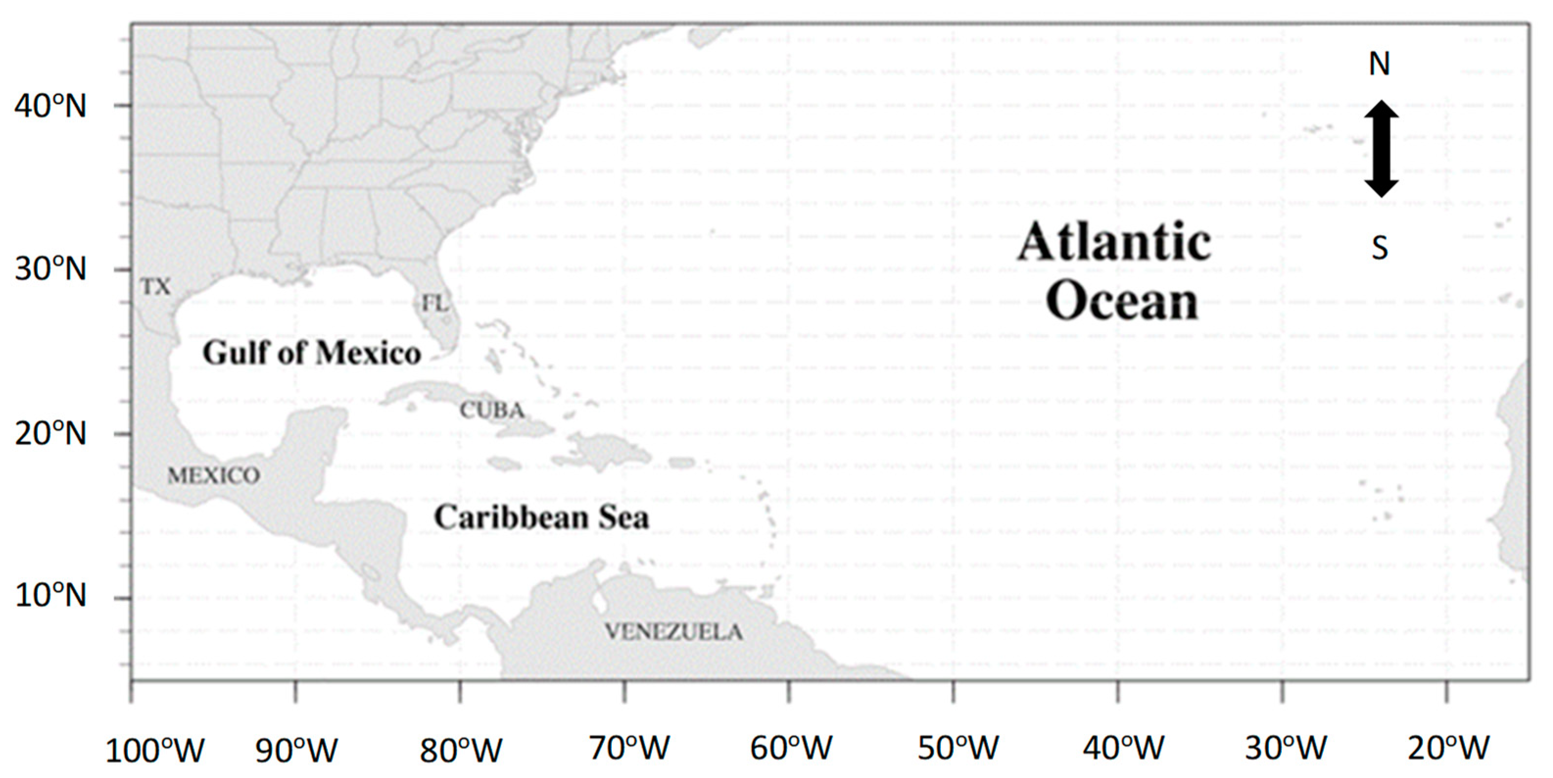
2.1. Data
2.2. Methods for Forecasting TC Counts
2.2.1. List of Statistical Models as Ensemble Members
- Partition data into windows, w = 39 for SWCV and no window for LOOCV (used here as the baseline);
- In each window, carry out the hierarchical clustering analysis and select the ten primary predictors; construct the model with Lasso using the ten covariates selected;
- Calculate the logarithm scores between the forecast and observed values;
- Compare scores with climatology using the mean likelihood skill score ().
2.2.2. Machine Learning Based Linear Combination of Statistical Models to Produce Ensemble Models
- Divide the data into 39 windows with 31 years in each window. The first 30 years are used for training and validation is performed on the 31st year.
- In each window, construct a model: use the predictions from 9 statistical models for each of the 30 years as training set and apply the optimization techniques to learn weight parameters. Predict count for the 31st year using the trained ensemble model.
- Compare scores against climatology using the mean H value.
- Lasso optimization:where is the Lasso shrinkage parameter and is the norm of the weights in the ensemble model.
- Ridge optimization:where is the ridge shrinkage parameter and is the norm of the weights in the ensemble model.
- Linear regression:where is the true count for training years, of shape , is a matrix of shape where each row corresponds to the output counts of nine statistical models and is the weight vector of shape . For SWCV, in each window, whereas for LOOCV, . The minimum value for the objective function will be 0 if , but it is not always possible that will be in the column space of , and hence the linear regression method finds the orthogonal projection of into the column space of . Let the orthogonal projection of in the column space of be , then will be the weight that gives a minimum value for the given objective function such that no other weights can give a lower value for the function. In this way, we obtain the weights .
- Gradient descent:
3. Results
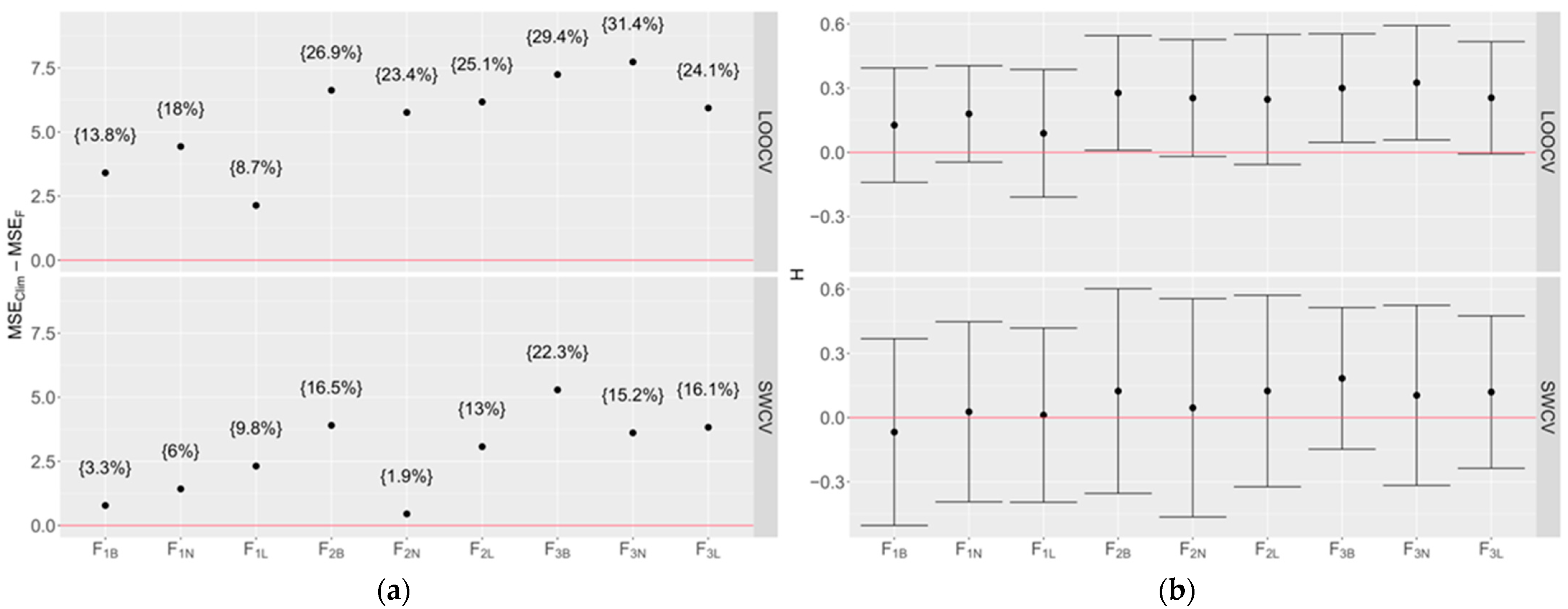
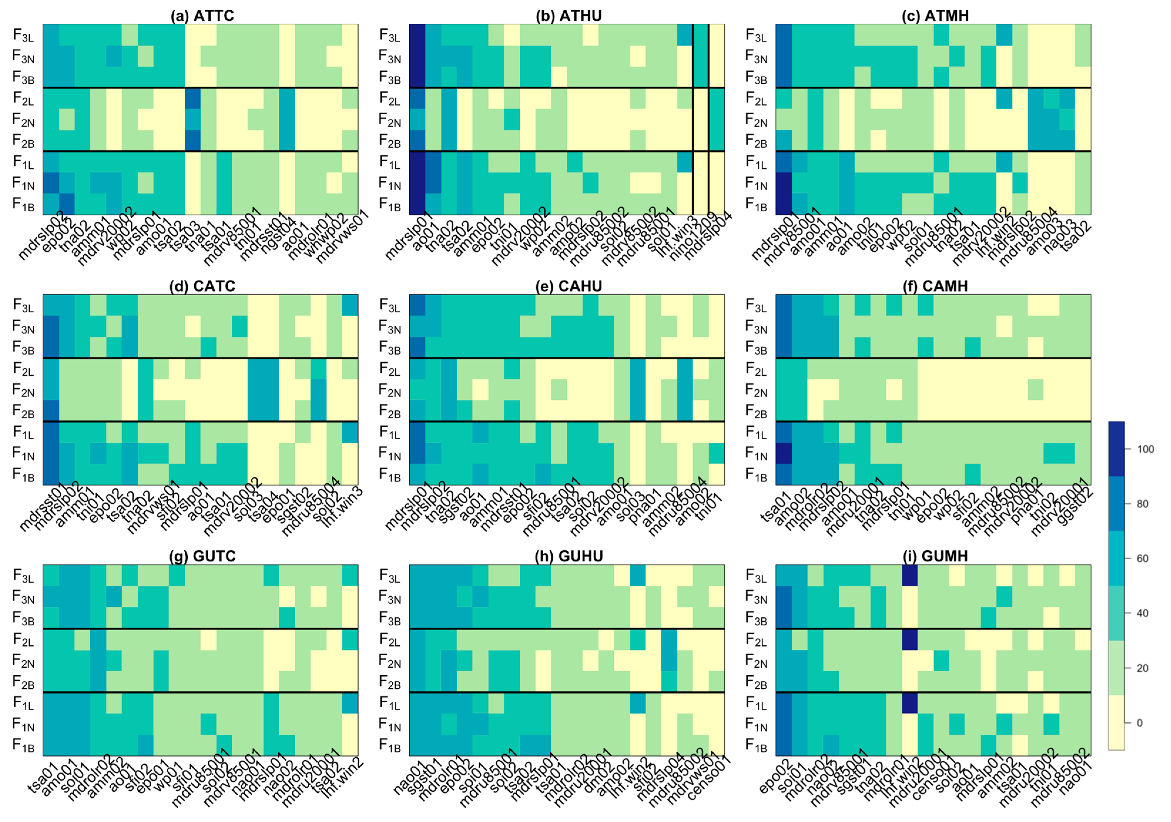
3.1. Results from Emsemble Members
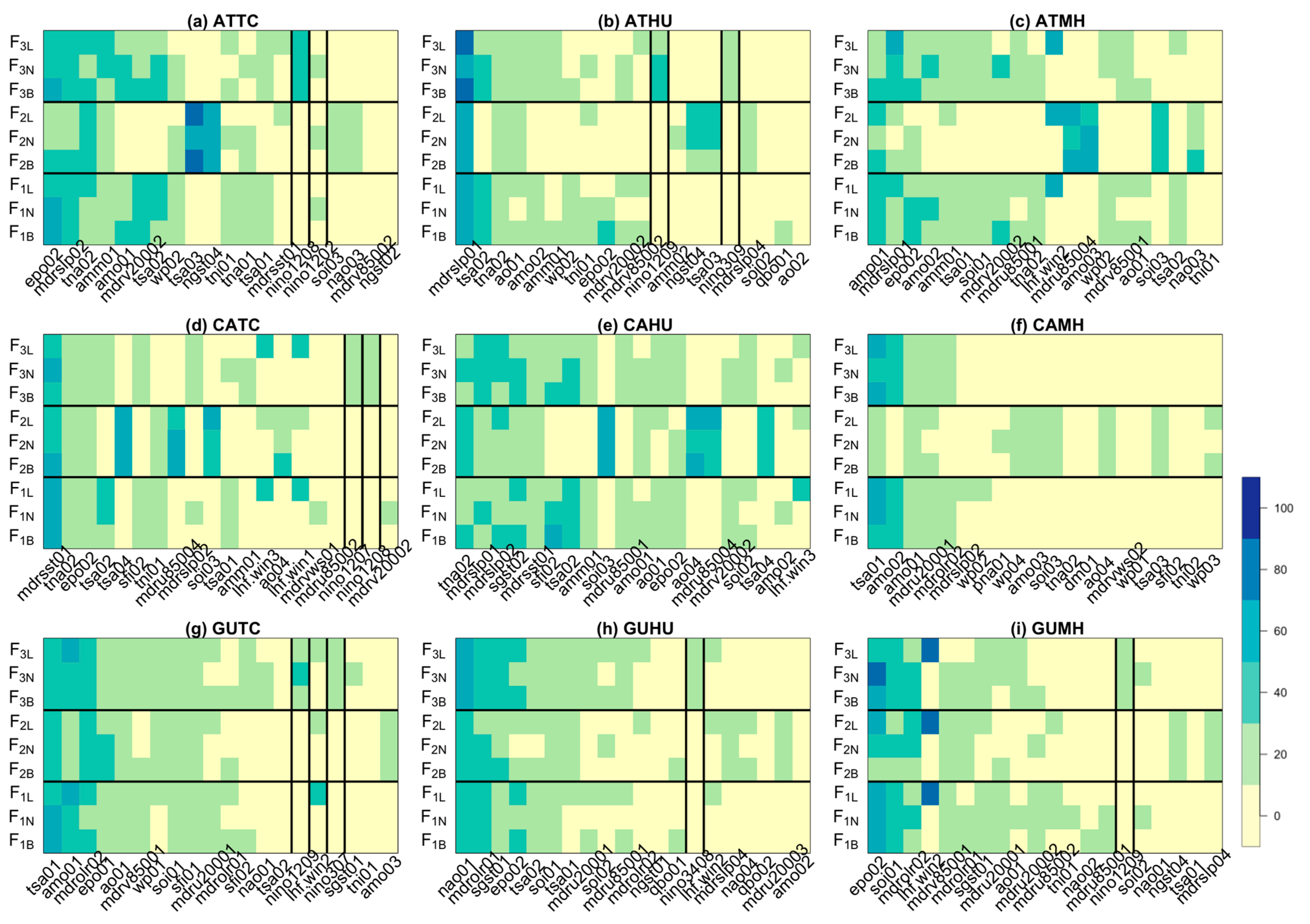
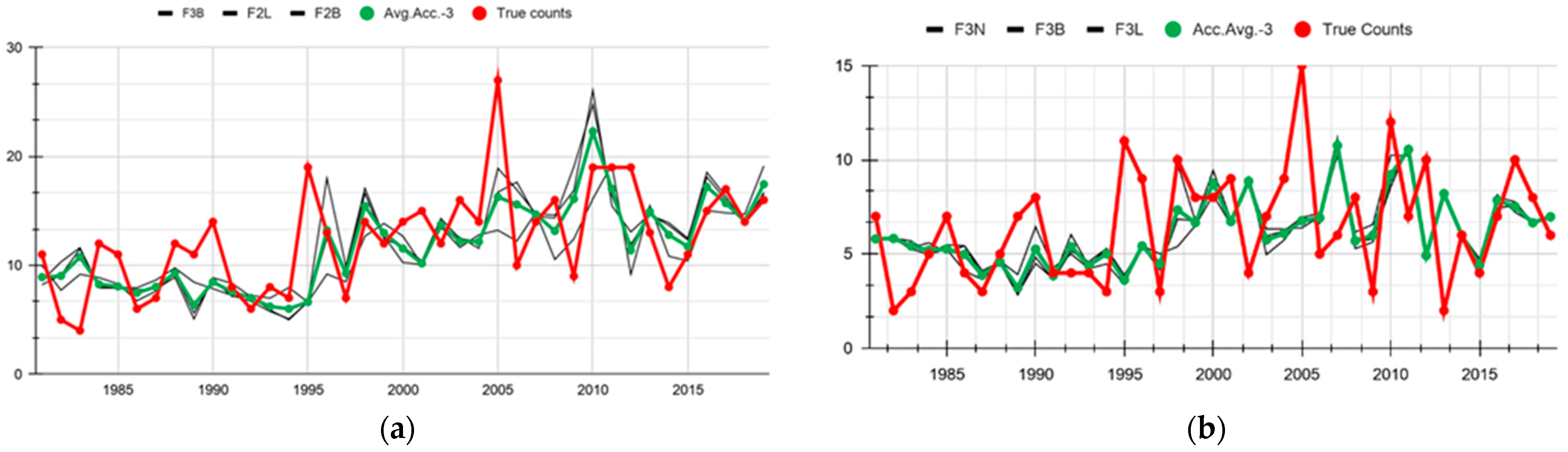
3.1.1. Results from Regression Models
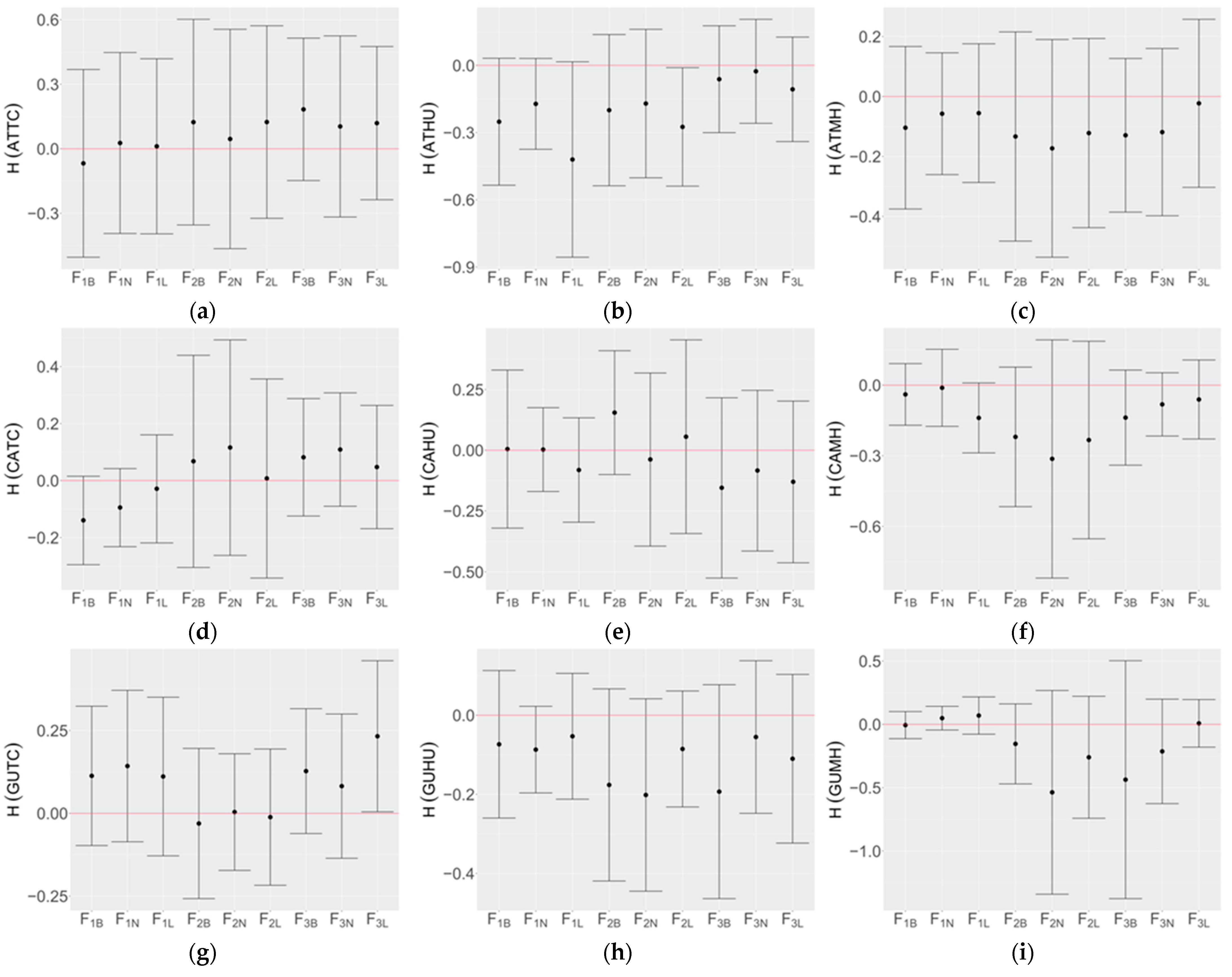
3.1.2. Potential Benefits of Multimodel Ensemble
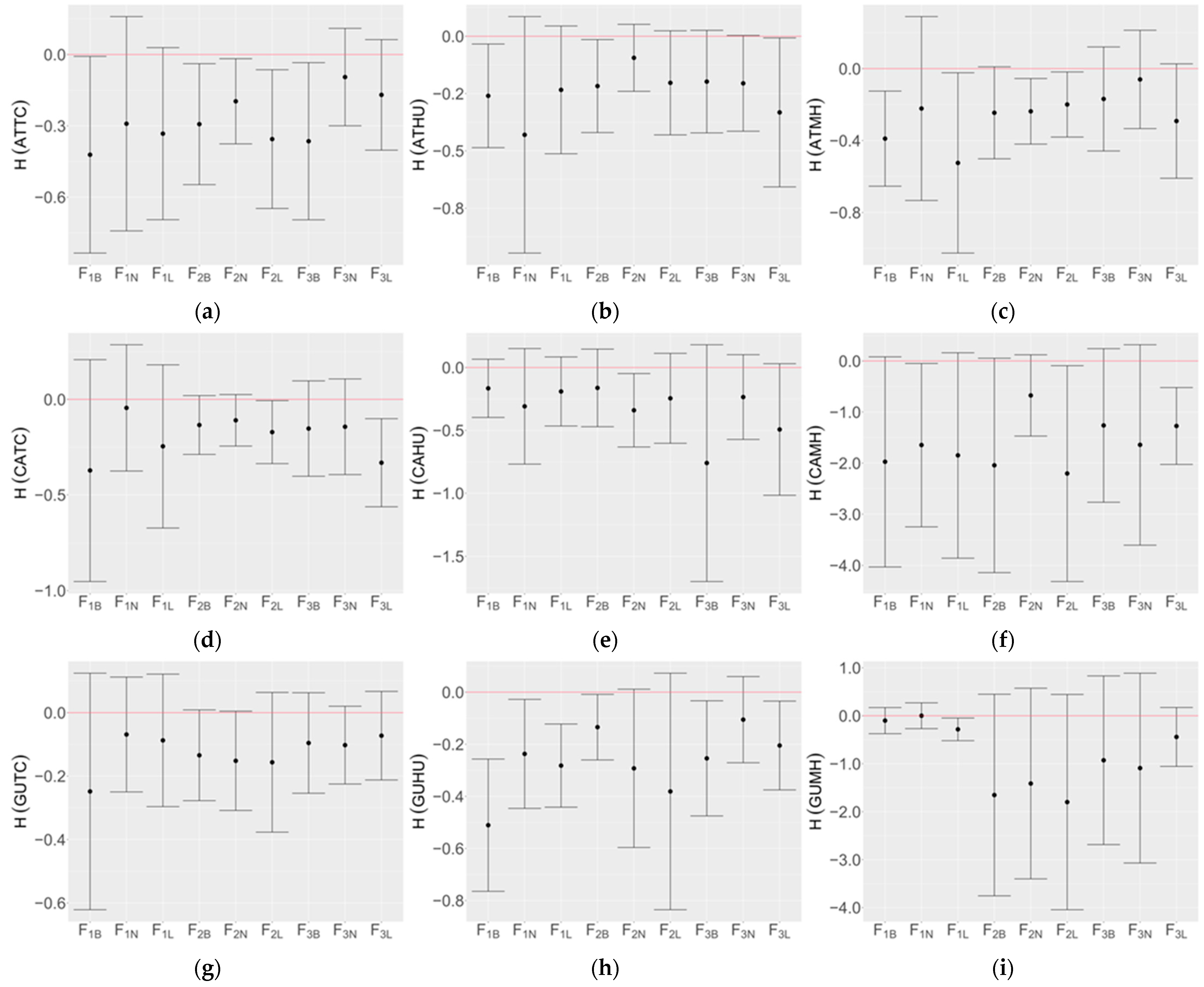
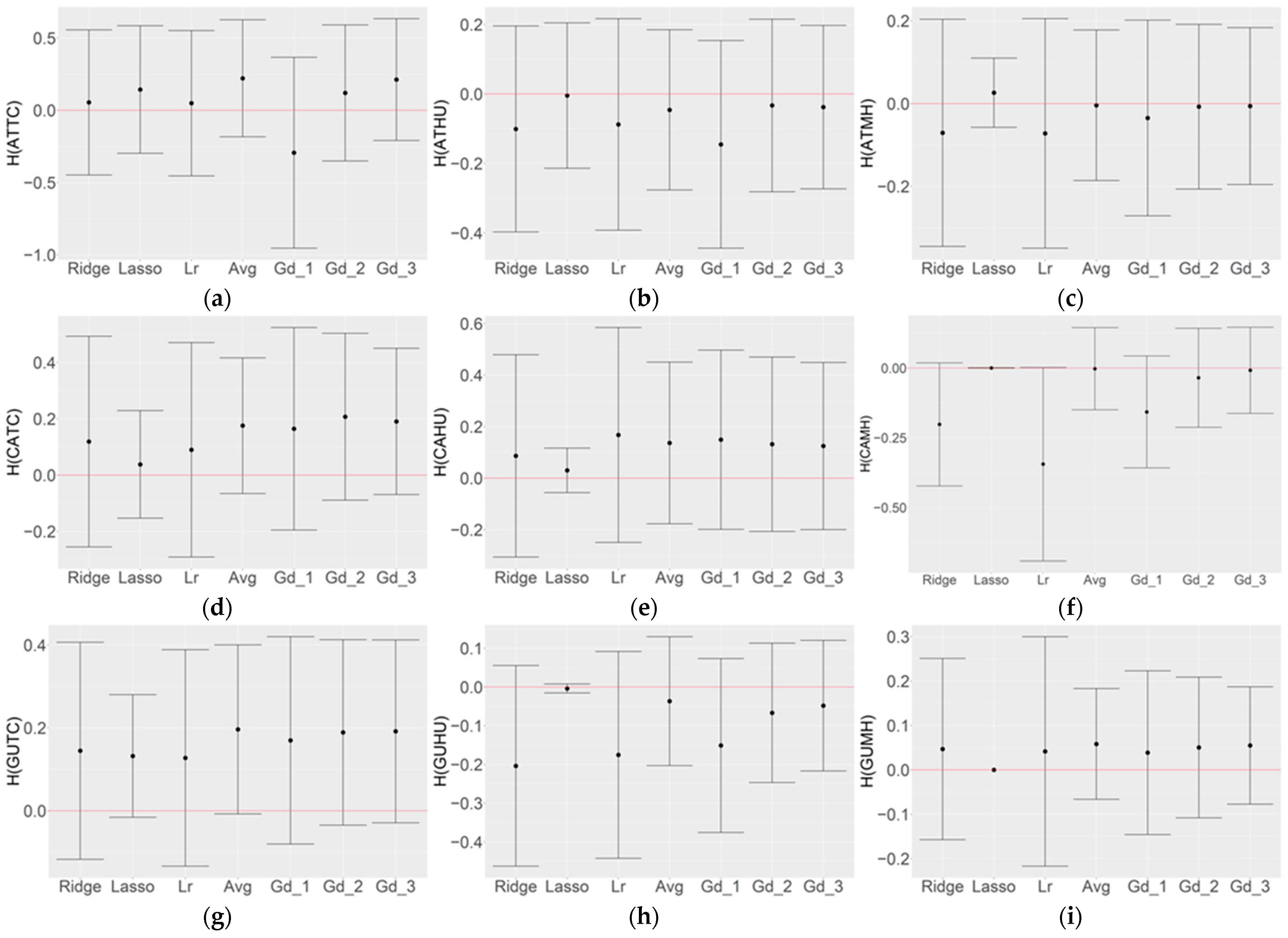
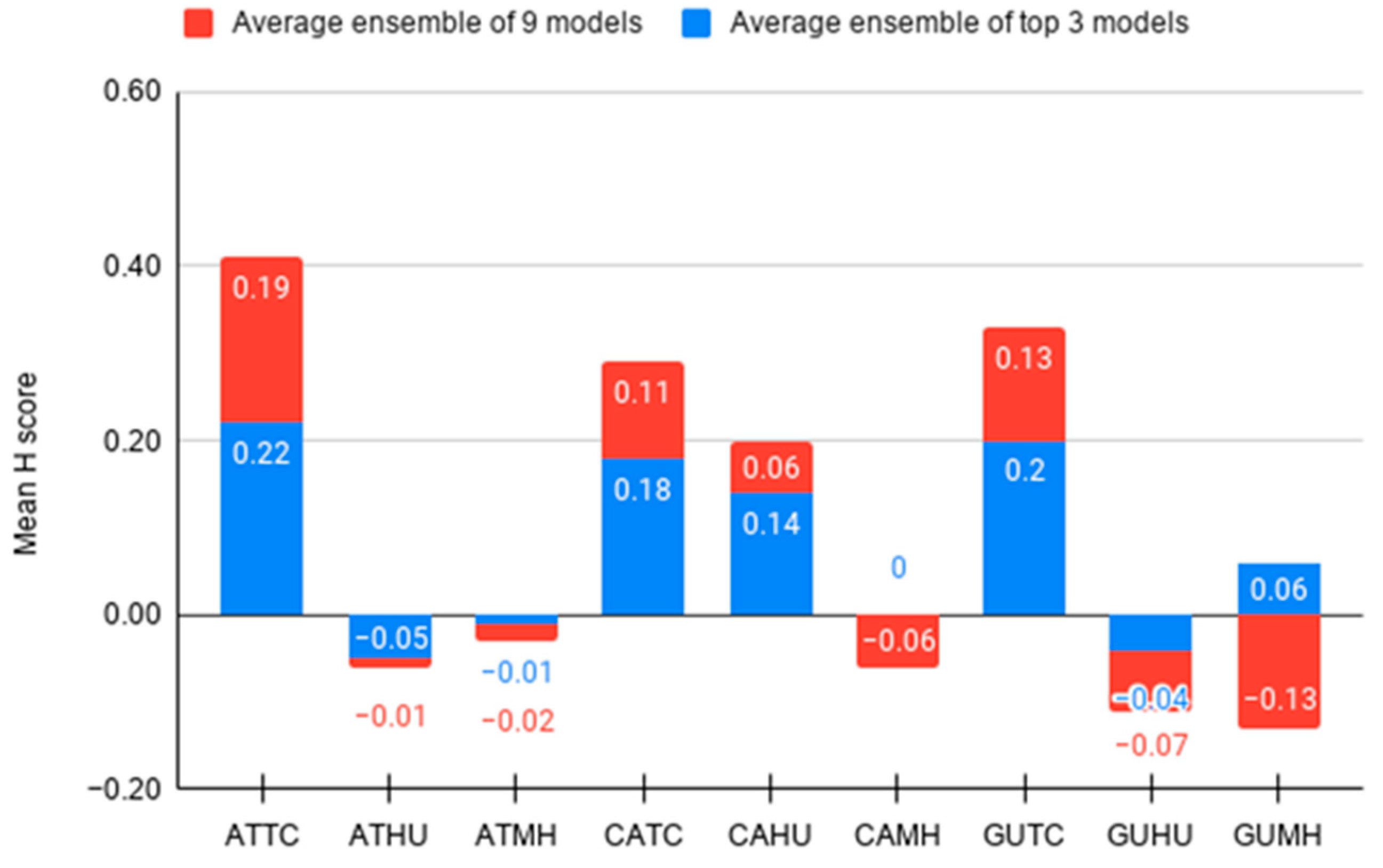
3.2. Comparison of Forecasts Using Simple Average Ensemble (SAE)
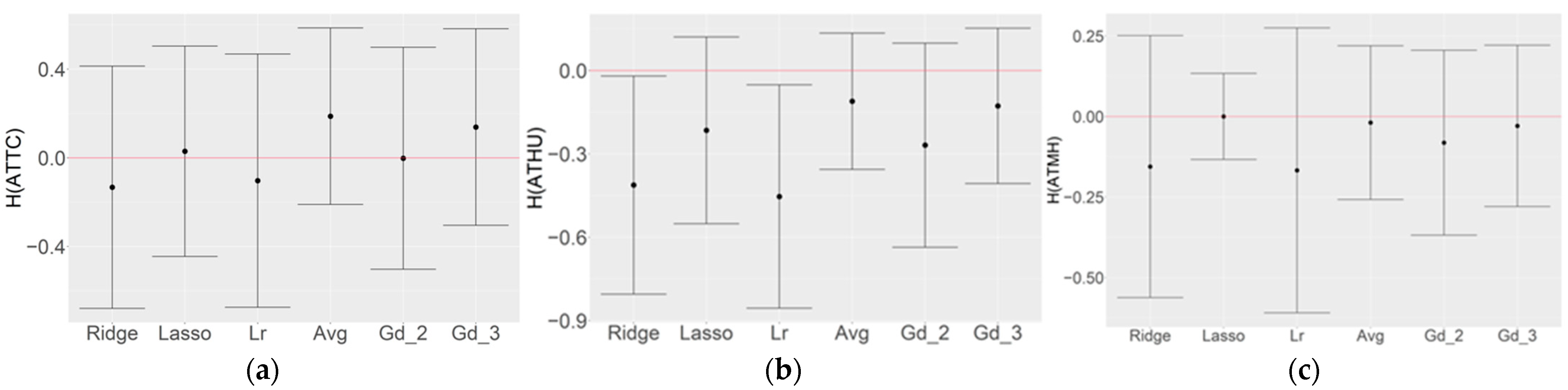
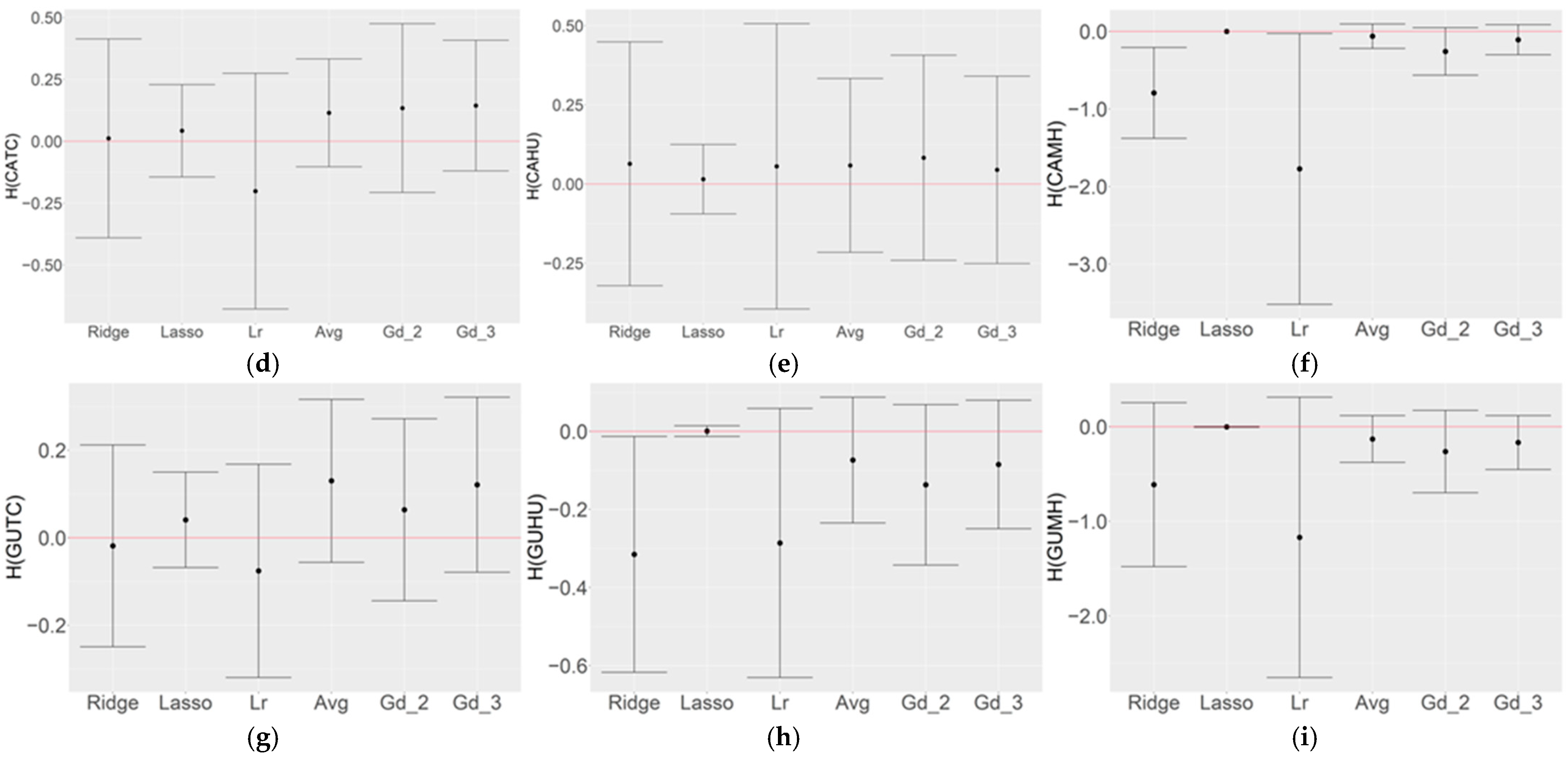
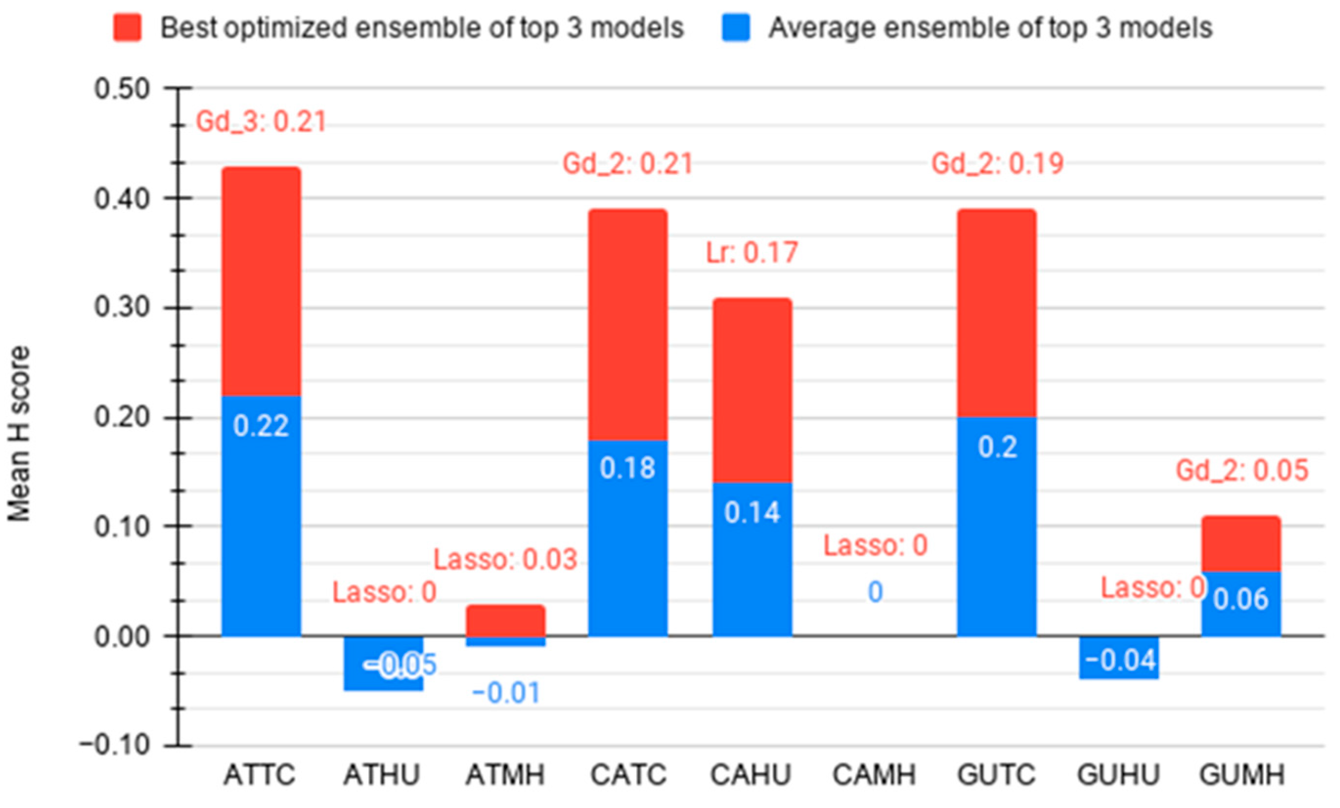
3.3. Optimization of Top Three Model Ensemble
4. Discussion
5. Conclusions
Author Contributions
Funding
Institutional Review Board Statement
Informed Consent Statement
Data Availability Statement
Acknowledgments
Conflicts of Interest
References
- Grinsted, A.; Ditlevsen, P.; Christensen, J.H. Normalized US hurricane damage estimates using area of total destruction, 1900-2018. Proc. Natl. Acad. Sci. USA 2019, 116, 23942–23946. [Google Scholar] [CrossRef] [PubMed]
- Doocy, S.; Dick, A.; Daniels, A.; Kirsch, T.D. The human impact of tropical cyclones: A historical review of events 1980-2009 and systematic literature review. PLOS Curr. Disasters 2013. [Google Scholar] [CrossRef] [PubMed]
- Smith, A.B.; Katz, R.W. US billion-dollar weather and climate disasters: Data sources, trends, accuracy and biases. Nat. Hazards 2013, 67, 387–410. [Google Scholar] [CrossRef]
- Gray, W.M. Summary of 1984 Atlantic Seasonal Tropical Cyclone Activity and Verification of Author’s Forecast (PDF) (Report); Colorado State University: Fort Collins, CO, USA, 2018. [Google Scholar]
- Gray, W.M. Atlantic seasonal hurricane frequency, Part I: El Niño and 30 mb quasi-biennial influence. Mon. Weather Rev. 1984, 112, 1649–1668. [Google Scholar] [CrossRef] [Green Version]
- Gray, W.M. Atlantic seasonal hurricane frequency, Part II: Forecasting its variability. Mon. Weather Rev. 1984, 112, 1669–1683. [Google Scholar] [CrossRef]
- Landsea, C.W.; Gray, W.M.; Mielke, P.W., Jr.; Berry, K.J. Seasonal forecasting of Atlantic hurricane activity. Weather 1994, 49, 273–284. [Google Scholar] [CrossRef]
- Keith, E.; Xie, L. Predicting Atlantic Tropical Cyclone Seasonal Activity in April. Weather Forecast. 2009, 24, 436–455. [Google Scholar] [CrossRef]
- Camargo, S.J.; Wing, A.A. Tropical cyclones in climate models. Wiley Interdiscip. Rev. Clim. Chang. 2005, 7, 211–237. [Google Scholar] [CrossRef]
- Klotzbach, P.J.; Caron, L.-P.; Bell, M.M. A statistical/dynamical model for North Atlantic seasonal hurricane prediction. Geophys. Res. Lett. 2020, 47. [Google Scholar] [CrossRef]
- Vecchi, G.A.; Zhao, M.; Wang, H.; Villarini, G.; Rosati, A.; Kumar, A.; Held, I.M.; Gudgel, R. Statistical–dynamical predictions of seasonal North Atlantic hurricane activity. Mon. Weather Rev. 2011, 139, 1070–1082. [Google Scholar] [CrossRef]
- Kim, H.-M.; Webster, P.J. Extended-range seasonal hurricane forecasts for the North Atlantic with a hybrid dynamical-statistical model. Geophys. Res. Lett. 2010, 37, L21705. [Google Scholar] [CrossRef] [Green Version]
- Wang, H.; Schemm, J.-K.E.; Wang, W.; Long, L.; Chelliah, M.; Bell, G.D.; Peng, P. Statistical Forecast Model for Atlantic Seasonal Hurricane Activity Based on the NCEP Dynamical Seasonal Forecast. J. Clim. 2009, 22, 4481–4500. [Google Scholar] [CrossRef]
- How Accurate are Pre-Season Hurricane Landfall Forecasts? Available online: https://www.washingtonpost.com/news/capital-weather-gang/wp/2013/04/23/how-accurate-are-pre-season-hurricane-landfall-forecasts/ (accessed on 26 February 2021).
- Klotzbach, P.J.; Saunders, M.A.; Bell, G.D.; Blake, E.S. North Atlantic Seasonal Hurricane Prediction. In Climate Extremes: Patterns and Mechanisms, Geophysical Monograph 226; Wang, S.-S., Yoon, J.-H., Funk, C.C., Gillies, R.R., Eds.; American Geophysical Union: Washington, DC, USA; John Wiley & Sons: Hoboken, NJ, USA, 2017. [Google Scholar] [CrossRef]
- Blake, E.B.; Gibney, E.J.; Brown, D.P.; Mainelli, M.; Franklin, J.L.; Kimberlain, T.B.; Hammer, G.R. Tropical Cyclones of the eastern North Pacific Ocean, 1949–2006. In Historical Climatology Series; National Climatic Data Center: Miami, FL, USA, 2008; Volume 2–6, in publication. [Google Scholar]
- Klotzbach, P.J.; Gray, W.M. Updated 6–11-Month Prediction of Atlantic Basin Seasonal Hurricane Activity. Weather Forecast. 2004, 19, 917–934. [Google Scholar] [CrossRef] [Green Version]
- Emanuel, K.; Fondriest, F.; Kossin, J. Potential Economic Value of Seasonal Hurricane Forecasts. Weather Clim. Soc. 2012, 4, 110–117. [Google Scholar] [CrossRef]
- Palmer, T.N. Predicting uncertainty in forecasts of weather and climate. Rep. Prog. Phys. 1999, 63. [Google Scholar] [CrossRef] [Green Version]
- Slingo, J.; Palmer, T. Uncertainty in weather and climate prediction. Phil. Trans. R. Soc. A. 2011, 369, 4751–4767. [Google Scholar] [CrossRef]
- Hewage, P.; Trovati, M.; Pereira, E.; Behera, A. Deep learning-based effective fine-grained weather forecasting model. Pattern Anal. Appl. 2021, 24, 343–366. [Google Scholar] [CrossRef]
- Scher, S.; Messori, G. Predicting weather forecast uncertainty with machine learning. Q. J. R Meteorol. Soc. 2018, 144, 2830–2841. [Google Scholar] [CrossRef]
- Rasp, S.; Lerch, S. Neural Networks for Postprocessing Ensemble Weather Forecasts. Mon. Weather Rev. 2021, 146, 3885–3900. Available online: https://journals.ametsoc.org/view/journals/mwre/146/11/mwr-d-18-0187.1.xml (accessed on 26 February 2021).
- Krasnopolsky, V.M.; Lin, Y. A Neural Network Nonlinear Multimodel Ensemble to Improve Precipitation Forecasts over Continental US. Adv. Meteorol. 2018, 2012, 649450. [Google Scholar] [CrossRef]
- Jagger, T.H.; Elsner, J.B. A Consensus Model for Seasonal Hurricane Prediction. J. Clim. 2010, 23, 6090–6099. [Google Scholar] [CrossRef]
- Richmana, M.B.; Lesliea, L.M.; Ramsay, H.A.; Klotzbach, P.J. Reducing Tropical Cyclone Prediction Errors Using Machine Learning Approaches. Procedia Comput. Sci. 2015. [Google Scholar] [CrossRef]
- Jarvinen, B.R.; Neumann, C.J.; Davis, M.A.S. A Tropical Cyclone Data Tape for the North Atlantic Basin, 1886–1983: Contents, Limitations, and Uses; NOAA Technical Memorandum NWS NHC 22: Coral Gables, FL, USA, 1984; p. 21.
- Leetmaa, A.; Reynolds, R.; Jenne, R.; Josepht, D. The NCEP/NCAR 40-year reanalysis project. Bull. Amer. Meteor. Soc. 1996, 77, 437–470. [Google Scholar]
- Córdoba, M.A.; Fuentes, M.; Guinness, J.; Xie, L. Verification of Statistical Seasonal Tropical Cyclone Forecast. Zenodo 2019. [Google Scholar] [CrossRef]
- Murtagh, F.; Legendre, P. Ward’s hierarchical agglomerative clustering method: Which algorithms implement Ward’s criterion? J. Classif. 2014, 31, 274–295. [Google Scholar] [CrossRef] [Green Version]


| Response Variable | Region | Definitions |
|---|---|---|
| ATTC | North Atlantic Basin | Atlantic Tropical Cyclones: counts of tropical storms, and hurricanes in North Atlantic |
| ATHU | Atlantic Hurricanes: counts of hurricanes in North Atlantic | |
| ATMH | Atlantic Major Hurricanes: counts of major hurricanes in North Atlantic | |
| CATC | Caribbean Sea | Caribbean Sea Tropical Cyclones: counts of tropical storms and hurricanes in Caribbean Sea |
| CAHU | Caribbean Sea Hurricanes: counts of hurricanes in Caribbean Sea | |
| CAMH | Caribbean Sea Major Hurricanes: counts of major hurricanes in Caribbean Sea | |
| GUTC | Gulf of Mexico | Gulf of Mexico Tropical Cyclones: counts of tropical storms and hurricanes in Gulf of Mexico |
| GUHU | Gulf of Mexico Hurricanes: counts of hurricanes in Gulf of Mexico | |
| GUMH | Gulf of Mexico Major Hurricanes: counts of major hurricanes in Gulf of Mexico |
| Model # | Time Domain | Covariates | |
|---|---|---|---|
| F1 (March Outlook) | F1B | January–February | Core |
| F1N | Core + NINO | ||
| F1L | Core + NINO + LHF | ||
| F2 (May Outlook) | F2B | January–April | Core |
| F2N | Core + NINO | ||
| F2L | Core + NINO + LHF | ||
| F3 (March Outlook with ENSO JAS Forecast) | F3B | January–February + NINO JAS Forecast | Core |
| F3N | Core + NINO | ||
| F3L | Core + NINO + LHF | ||
| Climate Index | Climate Index Name | ||
| Core | AMM | Atlantic Meridional Mode | |
| AMO | Atlantic Multidecadal Oscillation | ||
| AO | Arctic Oscillation | ||
| CENSO | Bivariate ENSO (El Niño–Southern Oscillation) time series | ||
| DM | Atlantic Dipole Mode (DM = TNA – TSA) | ||
| EPO | East Pacific/North Pacific Oscillation index | ||
| GGST | Global Mean Land/Ocean Temperature index | ||
| NGST | North-Hemisphere Mean Land/Ocean Temperature index | ||
| SGST | South-Hemisphere Mean Land/Ocean Temperature index | ||
| MDRSST | Sea Surface Temperature averaged over Major Development Region (MDR) | ||
| MDROLR | Top of Atmosphere Outgoing Longwave Radiation averaged over MDR | ||
| MDRSLP | Sea Level Pressure averaged over MDR | ||
| MDRU200 | Zonal Wind at 200 hPa averaged over MDR | ||
| MDRV200 | Meridional Wind at 200 hPa averaged over MDR | ||
| MDRU850 | Zonal Wind at 850 hPa averaged over MDR | ||
| MDRV850 | Meridional Wind at 850 hPa averaged over MDR | ||
| MDRVWS | Vertical Wind Shear averaged over MDR | ||
| NAO | North Atlantic Oscillation | ||
| PDO | Pacific Decadal Oscillation | ||
| PNA | Pacific North American index | ||
| QBO | Quasi-Biennial Oscillation | ||
| SFI | Solar Flux (10.7 cm) | ||
| SOI | Southern Oscillation Index | ||
| TNI | Trans-Niño Index | ||
| TNA | Tropical Northern Atlantic index | ||
| TSA | Tropical Southern Atlantic index | ||
| WHWP | Western Hemisphere Warm Pool | ||
| WP | Western Pacific index | ||
| NINO | MEI | Multivariate ENSO Index | |
| NINO12 | Extreme Eastern Tropical Pacific SST (0–10° S, 90° W–80° W) | ||
| NINO3 | Eastern Tropical Pacific SST (5° N–5° S, 150–90° W) | ||
| NINO34 | East Central Tropical Pacific SST (5° N–5° S, 170–120° W) | ||
| NINO4 | Central Tropical Pacific SST (5° N–5° S, 160° E–150° W) | ||
| LHF | LHF.WIN | LHF EOF Scores for Winter | |
| F | 1 | 2 | 3 | 4 | 5 |
|---|---|---|---|---|---|
| F1B | EPO02 (56) | MDRV20002 (38) | MDRSLP02 (36) | AMO01 (36) | TNA02 (33) |
| F1N | EPO02 (54) | TSA02 (46) | MDRV20002 (44) | MDRSLP02 (36) | AMO01 (33) |
| F1L | EPO02 (44) | MDRSLP02 (41) | TNA02 (36) | MDRV20002 (36) | TSA02 (36) |
| F2B | TSA03 (72) | NGST04 (54) | TNA02 (38) | EPO02 (36) | MDRSLP02 (36) |
| F2N | TSA03 (67) | NGST04 (59) | TNA02 (41) | EPO02 (31) | NINO1202 (31) |
| F2L | TSA03 (69) | NGST04 (51) | TNA02 (44) | EPO02 (33) | MDRSLP02 (28) |
| F3B | EPO02 (51) | MDRSLP02 (41) | NINO1208 (41) | TNA02 (36) | AMO01 (36) |
| F3N | EPO02 (49) | MDRSLP02 (38) | TSA02 (38) | NINO1208 (38) | AMM01 (36) |
| F3L | EPO02 (44) | AMM01 (44) | MDRSLP02 (41) | TNA02 (36) | NINO1208 (36) |
| F | 1 | 2 | 3 | 4 | 5 |
|---|---|---|---|---|---|
| F1B | EPO02 (69) | MDRSLP02 (67) | MDRV20002 (51) | MDRSLP01 (49) | TSA02 (41) |
| F1N | MDRSLP02 (77) | EPO02 (67) | MDRV20002 (56) | AMM01 (54) | TSA02 (46) |
| F1L | MDRSLP02 (67) | LHF.WIN3 (51) | EPO02 (49) | AMM01 (49) | MDRV20002 (49) |
| F2B | TSA03 (74) | NGST04 (54) | TNA02 (49) | NAO03 (41) | MDRSLP02 (38) |
| F2N | TSA03 (67) | NGST04 (59) | TNA02 (44) | MDRSLP02 (41) | AMO04 (41) |
| F2L | TSA03 (72) | NGST04 (54) | TNA02 (46) | MDRSLP02 (38) | NAO03 (38) |
| F3B | EPO02 (59) | MDRSLP02 (56) | MDRV20002 (49) | NINO1208 (44) | TSA02 (41) |
| F3N | MDRSLP02 (67) | EPO02 (56) | MDRV20002 (51) | AMM01 (49) | WP02 (49) |
| F3L | MDRSLP02 (54) | EPO02 (46) | AMM01 (46) | LHF.WIN3 (46) | MDRV20002 (44) |
| Rank | ATTC | ATHU | ATMH | CATC | CAHU | CAMH | GUTC | GUHU | GUMH |
|---|---|---|---|---|---|---|---|---|---|
| 1 | F3B | F3N | F3L | F2N | F2B | F1N | F3L | F1L | F1L |
| 2 | F2L | F3B | F1L | F3N | F2L | F1B | F1N | F3N | F1N |
| 3 | F2B | F3L | F1N | F3B | F1B | F3L | F3B | F1B | F3L |
| 4 | F3L | F2N | F1B | F2B | F1N | F3N | F1B | F2L | F1B |
| 5 | F3N | F1N | F3N | F3L | F2N | F3B | F1L | F1N | F2B |
| 6 | F2N | F2B | F2L | F2L | F1L | F1L | F3N | F3L | F3N |
| 7 | F1N | F2L | F3B | F1L | F3N | F2B | F2N | F2B | F2L |
| 8 | F1L | F1B | F2B | F1N | F3L | F2L | F2L | F3B | F3B |
| 9 | F1B | F1L | F2N | F1B | F3B | F2N | F2B | F2N | F2N |
| Rank | ATTC | ATHU | ATMH | CATC | CAHU | CAMH | GUTC | GUHU | GUMH |
|---|---|---|---|---|---|---|---|---|---|
| 1 | F2B | F2N | F3N | F3L | F2B | F1B | F1N | F1L | F1L |
| 2 | F3N | F2L | F3B | F3B | F2L | F3N | F2L | F3N | F3L |
| 3 | F2N | F2B | F3L | F2N | F2N | F3B | F1B | F3B | F2L |
| 4 | F2L | F3L | F1N | F3N | F3L | F3L | F3B | F3L | F1B |
| 5 | F3B | F3B | F1L | F1B | F3B | F1N | F2B | F1N | F3B |
| 6 | F3L | F3N | F1B | F1N | F3N | F2L | F3N | F1B | F3N |
| 7 | F1N | F1N | F2L | F2B | F1L | F1L | F1L | F2N | F2N |
| 8 | F1B | F1B | F2N | F2L | F1N | F2N | F3L | F2L | F1N |
| 9 | F1L | F1L | F2B | F2N | F1B | F2B | F2N | F2B | F2B |
| Response | 1 | 2 | 3 | 4 | 5 | 6 | 7 | 8 | 9 |
|---|---|---|---|---|---|---|---|---|---|
| ATTC | 0.18 | 0.23 | 0.22 | 0.23 | 0.23 | 0.22 | 0.21 | 0.20 | 0.19 |
| ATHU | −0.03 | 0.00 | 0.00 | −0.04 | −0.05 | −0.05 | −0.07 | −0.09 | −0.11 |
| ATMH | −0.02 | 0.03 | 0.03 | 0.02 | −0.01 | −0.02 | −0.02 | −0.01 | 0.00 |
| CATC | 0.12 | 0.20 | 0.21 | 0.20 | 0.20 | 0.18 | 0.17 | 0.16 | 0.14 |
| CAHU | 0.15 | 0.19 | 0.17 | 0.21 | 0.17 | 0.13 | 0.18 | 0.10 | 0.08 |
| CAMH | −0.01 | 0.00 | 0.00 | 0.00 | 0.00 | 0.00 | 0.00 | 0.00 | 0.00 |
| GUTC | 0.23 | 0.22 | 0.20 | 0.19 | 0.18 | 0.17 | 0.16 | 0.14 | 0.13 |
| GUHU | −0.05 | 0.00 | 0.00 | 0.00 | 0.00 | 0.00 | 0.00 | 0.00 | 0.00 |
| GUMH | 0.07 | 0.09 | 0.06 | 0.08 | 0.02 | 0.00 | 0.00 | 0.00 | 0.00 |
Publisher’s Note: MDPI stays neutral with regard to jurisdictional claims in published maps and institutional affiliations. |
© 2021 by the authors. Licensee MDPI, Basel, Switzerland. This article is an open access article distributed under the terms and conditions of the Creative Commons Attribution (CC BY) license (https://creativecommons.org/licenses/by/4.0/).
Share and Cite
Sun, X.; Xie, L.; Shah, S.U.; Shen, X. A Machine Learning Based Ensemble Forecasting Optimization Algorithm for Preseason Prediction of Atlantic Hurricane Activity. Atmosphere 2021, 12, 522. https://doi.org/10.3390/atmos12040522
Sun X, Xie L, Shah SU, Shen X. A Machine Learning Based Ensemble Forecasting Optimization Algorithm for Preseason Prediction of Atlantic Hurricane Activity. Atmosphere. 2021; 12(4):522. https://doi.org/10.3390/atmos12040522
Chicago/Turabian StyleSun, Xia, Lian Xie, Shahil Umeshkumar Shah, and Xipeng Shen. 2021. "A Machine Learning Based Ensemble Forecasting Optimization Algorithm for Preseason Prediction of Atlantic Hurricane Activity" Atmosphere 12, no. 4: 522. https://doi.org/10.3390/atmos12040522