Article

Associations between Exposure to Industrial Air Pollution and Prevalence of Asthma and Atopic Diseases in Haifa Bay Area

1
Braun School of Public Health and Community Medicine, The Hebrew University of Jerusalem—Hadassah, Jerusalem 9112102, Israel
2
Faculty of Civil and Environmental Engineering, Technion, Haifa 3200003, Israel
3
Technion Center of Excellence in Exposure Sciences and Environmental Health (TCEEH), Haifa 3200003, Israel
4
The Cystic Fibrosis Center, Rambam Medical Center, Haifa 3109601, Israel
5
Pediatric Pulmonology Unit, Department of Pediatrics, Hadassah-Hebrew University Medical Center, Jerusalem 9112102, Israel
6
The Wohl Institute for Translational Medicine, Hadassah-Hebrew University Medical Center, Jerusalem 9112102, Israel
7
Faculty of Medicine, Hebrew University of Jerusalem, Jerusalem 9112102, Israel
8
Israel Center for Disease Control, Israel Ministry of Health, Jerusalem 9446724, Israel
9
School of Public Health, University of Haifa, Haifa 3109601, Israel
10
Israel Defense Forces Medical Corps, Ramat Gan 5262000, Israel
11
Sackler Faculty of Medicine, Tel Aviv University, Tel Aviv 6997801, Israel
12
Central Management, Sheba Medical Center, Tel Hashomer, Ramat Gan 5262000, Israel
13
Department of Geography, The Hebrew University of Jerusalem, Jerusalem 9190501, Israel
14
Remote Sensing Research Centre, School of Earth and Environmental Sciences, University of Queensland, Brisbane, QLD 4072, Australia
15
Department of Military Medicine, Faculty of Medicine, Hebrew University of Jerusalem, Jerusalem 9112102, Israel
16
Institute of Endocrinology, Sheba Medical Center, Tel Hashomer, Ramat Gan 5262000, Israel
*
Author to whom correspondence should be addressed.
This author has passed away.
Atmosphere 2021, 12(4), 516; https://doi.org/10.3390/atmos12040516
Submission received: 5 March 2021 / Revised: 30 March 2021 / Accepted: 12 April 2021 / Published: 19 April 2021
(This article belongs to the Special Issue Air Pollution and Human Exposures in Israel)

Abstract

:
Haifa Bay Area (HBA) contains Israel’s principal industrial area, and there are substantial public concerns about health effects from its emissions. We aimed to examine associations between exposure to air pollution from HBA industrial area with prevalent asthma and other atopic diseases at age 17. This is a cross-sectional study. The study population included all adolescents born in Israel and whose medical status was evaluated for mandatory military recruitment by the Israeli medical corps during 1967–2017. We analyzed prevalent asthma, allergic rhinitis, atopic dermatitis, and rhinoconjunctivitis. We estimated exposure to industrial air pollution by a kriging interpolation of historical SO2 observations and adjusted the associations to the year of birth, SES, school orientation, and traffic pollution. The study population included n = 2,523,745 adolescents, among which 5.9% had prevalent asthma and 4.6% had allergic rhinitis. Residency in HBA was associated with a higher adjusted risk of asthma, compared with non-HBA residency. Still, this association was limited to the three lowest exposure categories, while the highest exposure group had the lowest adjusted risk. Sensitivity analyses and other atopic diseases presented similar results. These results do not provide support for causal relationships between HBA industry-related emissions and prevalent atopic diseases.

1. Introduction

Haifa Bay Area (HBA) is one of Israel’s largest metropolises and contains its principal industrial area. The latter includes heavy industry, such as refineries and a petrochemical complex, a power plant, petrol and chemical storage tanks, distribution centers, and many small industrial plants (such as metal processing, chemical and pharmaceutical factories, garages, printing houses, and others). In addition, the unique topography of the area results in complex local micrometeorological conditions that affect the atmospheric dispersion of emitted pollutants.
Air pollution measurements in HBA are not available for the period before the early 1980s. The combination of intense industrial activity and lack of emission control measures suggests elevated levels of various air pollutants in the 20th century. Anecdotal evidence can be found in an epidemiological study that reported very high monthly mean and maximal monthly concentrations of SO2 in 1982–1984 in two HBA locations [1]. The maximal concentrations exceeded the current hourly standard (350 µg/m3) in both locations almost every month in the study period. Despite a dramatic decline in the emissions of most of the criteria air pollutants, the current HBA’s emissions inventory is still very high in some cases and for specific pollutants. Specifically, the Haifa region volatile organic compounds (VOC) emissions are the largest in Israel per unit area.
An extensive air quality monitoring (AQM) array was established in HBA in the early-1980s. It has expanded since then to include about 20 stations, which observe various criteria pollutants: SO2, particulate matter (PM, including PM10 and PM2.5), CO, ozone, and nitrogen oxides (NOx). The AQM array was the first in Israel to include a four VOC analyzer for benzene, toluene, ethylbenzene, and xylene (BTEX) since the early 2000s in two stations and many more AQM stations since 2015. A nationwide biweekly sampling of about 15 additional VOCs commenced by the Ministry of Environmental Protection in the second decade of the 21st century. Since 2015 it has included eight locations in HBA and a different background site 20 km away. The samples are also analyzed for concentrations of seven metals in the particulate matter (arsenic, cadmium, chromium, lead, mercury, nickel, and vanadium).
Despite the high emissions inventory, the ambient concentrations of all the pollutants observed by HBA’s extensive AQM array are similar or lower than the corresponding concentrations in other major urban centers in Israel. They have been so since the early 2000s. Specifically, the concentration of NOx, the best proxy to ultrafine PM [2], is about 40% of those observed in Tel Aviv, the largest metropolis in Israel [2,3,4]. In addition, the concentrations of VOCs and particulate metals observed by the biweekly sampling are similar or lower than corresponding observations in the rest of the country.
In the long term, VOCs are mostly known for increasing the risk of various malignancies [5,6]. In the short term, and specifically for exposure through inhalation—which is the most relevant exposure pathway in the current context—VOCs such as BTEX, aldehydes, and PAHs irritate the respiratory tract in children [6,7,8,9], and mechanistic explanations for this effect are generally known [8,10]. Children are more sensitive to environmental pollution because their lungs are still developing, their ventilation rate is higher, their airways are smaller, and they spend more time outdoors. A previous report showed that HBA presents the highest pediatric hospitalizations incidence due to asthma in Israel (114.5 per 100,000 children: more than twice the Tel Aviv area incidence and 7-fold the Jerusalem area rate) [11]. High levels of environmental exposure to specific metals have deleterious clinical outcomes [12], and metal contents in aerosols are associated with asthma in several independent epidemiological studies [13,14].
There is substantial public concern about excess morbidity in HBA, particularly for malignant, cardiovascular, and respiratory diseases. Given that these illnesses are affected by chronic exposures, current morbidity may have been impacted by past exposures that no longer exist in the area. Therefore, to study factors that influenced current, recent, or past morbidity, one must obtain some exposure assessment based on historical measures.
Previous epidemiological studies mainly used variations of ecological study designs, in which both exposures and outcomes were assessed using aggregated measures, without any individual-level data [15,16,17,18,19]. One exception for this design is a study on cancer incidence in adults, in which individual-level cancer incidence data was used, but no exposure assessment was made [20]. Furthermore, these studies examined associations with criteria pollutants (such as NOx, SO2, or PM) but not with VOCs or metals. The ecological design in epidemiology is methodologically inferior since it is prone to the “ecological fallacy” [21] and is highly susceptible to confounding. It cannot be used to test epidemiological hypotheses, and its primary use in modern epidemiology is limited to generating new ideas. Besides, criteria pollutants do not represent the unique exposures at HBA and cannot be attributed to industrial emissions (SO2 is an exception to this under certain assumptions, as explained below). Therefore, the existing epidemiological literature on HBA cannot teach us much about the possible health effects of specific industrial HBA emissions on the HBA population.
Due to HBA complex topography and wind field, it is unknown how pollutant emissions disperse in space and whether exposure to industrial pollutant emissions has any health effects on HBA residents. These fundamental questions are highly dependent and require a new approach that will overcome three major obstacles. Firstly, most VOCs and toxic metals are rarely measured. The methods to measure them are technically complicated and expensive. Secondly, the complex topography of HBA and its effects on wind patterns make it very challenging to model spatial patterns of air pollutant concentrations. The cost of a full-scale, highly spatially resolved model is prohibitive, but simple dispersion models without data assimilation of AQM data are insufficient. Thirdly, emissions from the HBA industry changed with time, and even in the late 1990s, there was no substantial air monitoring.
This study examines associations between exposure to air pollution emitted by HBA industries with the prevalence of asthma and other atopic diseases at the age of 17. It estimates these associations using a new approach for exposure assessment. Accordingly, we have developed a new exposure model to estimate historical exposure to air pollution from the HBA industry. This model is based on historical SO2 measurements from when these measurements can be attributed to industrial sources in HBA. The study is unique since this exposure does not represent a specific pollutant but is meant to represent a mix of measured and unmeasured contaminants from the industrial area. The exposure estimates were linked to the Israeli medical corps database that included health examinations for all Israeli candidates for mandatory military service between 1967 and 2017.

2. Methods

2.1. Study Design and Study Population

This is a cross-sectional study. The study population included all adolescents aged 16–18 born in Israel and whose medical status was evaluated for mandatory military recruitment by the Israeli medical corps during 1967–2017 (n = 2,523,745). Ethical permission for the study was granted by the ethics committee of the medical corps institutional review board.

2.2. Outcome Assessment

Identifications of health outcomes at regional military recruitment centers have been described previously [22]. Briefly, as part of a medical assessment to mandatory military service, Israeli adolescents routinely undergo a medical evaluation approximately at the age of 17 years. The medical assessment includes a thorough review of medical history made by a physician and a physical examination. Abnormal findings are followed by additional tests and consultation, as appropriate. Subsequently, a specific standardized numerical code is assigned to each examinee to denote a medical diagnosis documented in a central database. This database was used recently in several epidemiological studies [22,23,24,25,26,27].
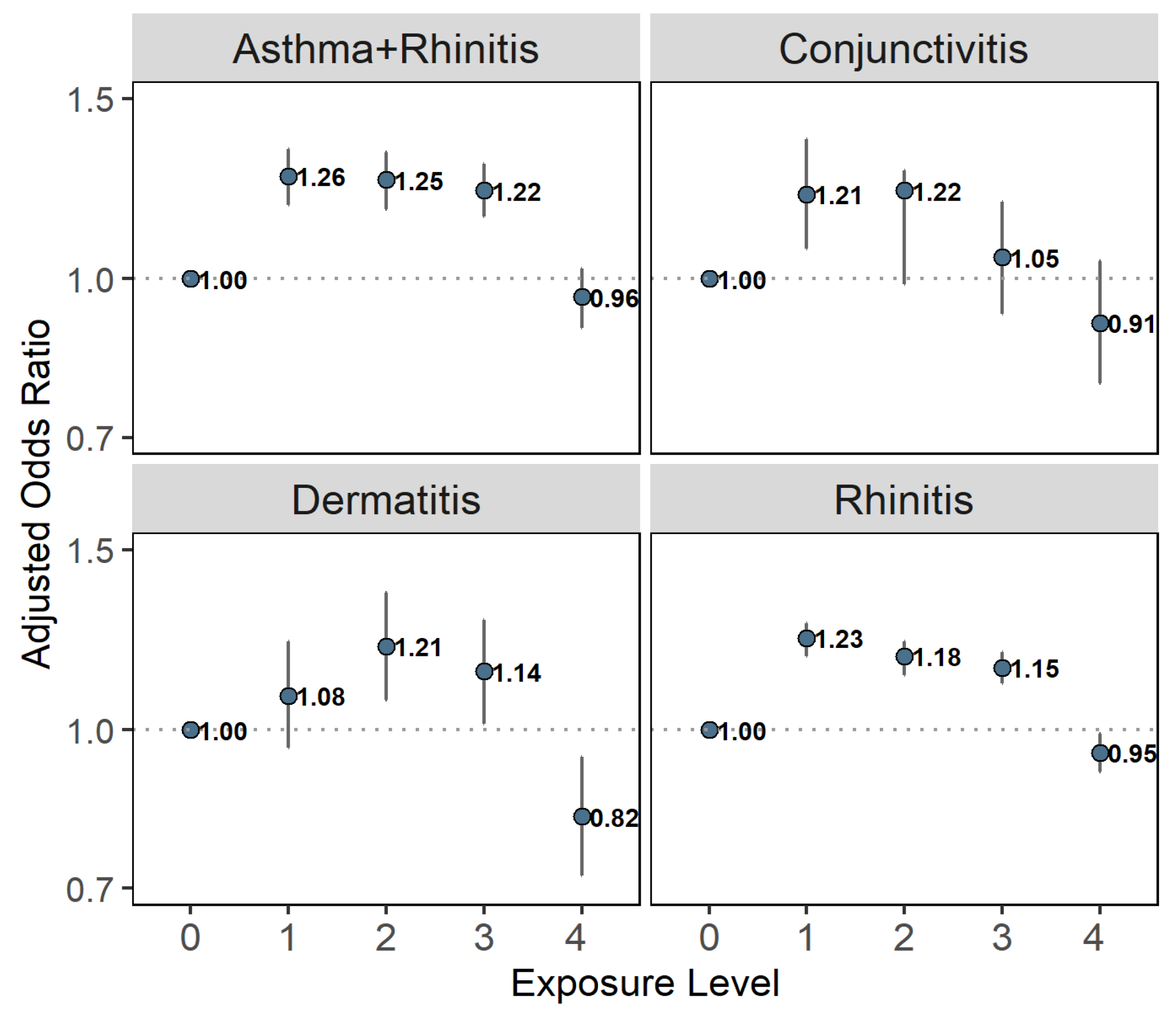
The health outcomes were prevalent asthma, allergic rhinitis, atopic dermatitis, and rhinoconjunctivitis for the current study. Asthma has been a reason for rejection from combat military service to noncombat services, hence suspected asthma cases are strictly evaluated by the medical corps. Subjects with a known diagnosis of these conditions were obliged to provide a documented diagnosis made by a relevant specialist (dermatologist, pulmonologist, or allergist) stating their current disease status and current medical treatment. Examinees suspected of having an undiagnosed illness at the time of medical evaluation were referred for further medical assessment by the relevant specialist. An appropriate board-specific specialist approved any diagnostic code for the study outcomes [28].

2.3. Exposure Data

The AQM array in HBA included during the study period up to 26 stations, which observed selected ambient pollutants and meteorological variables. This work uses only the SO2 concentrations data observed when the number of SO2 analyzers reached its maximum of 21. Figures S1 and S2 show the 21 SO2 monitoring sites’ locations and the number of stations that monitored SO2 per year in 1991–2016.
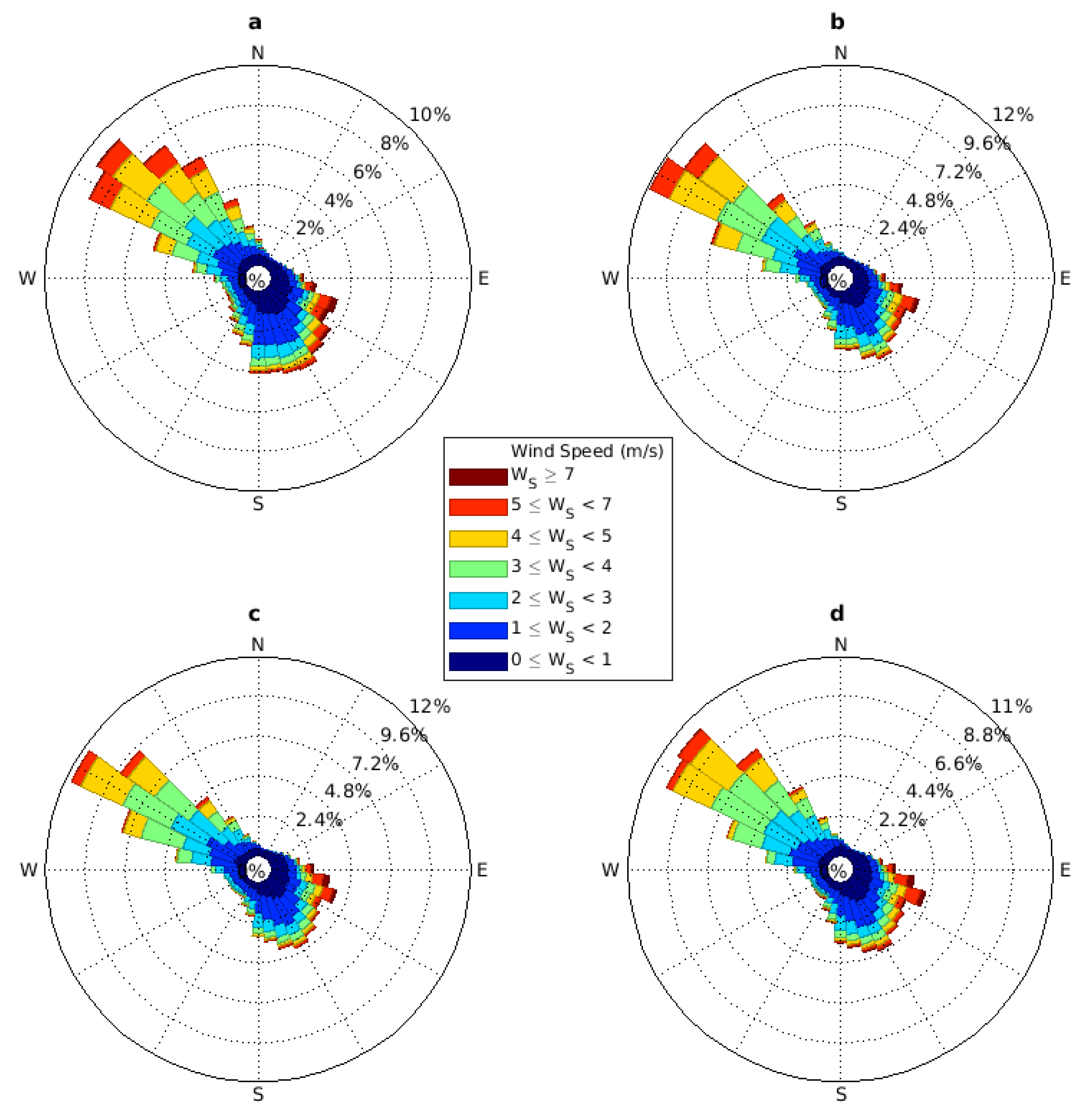
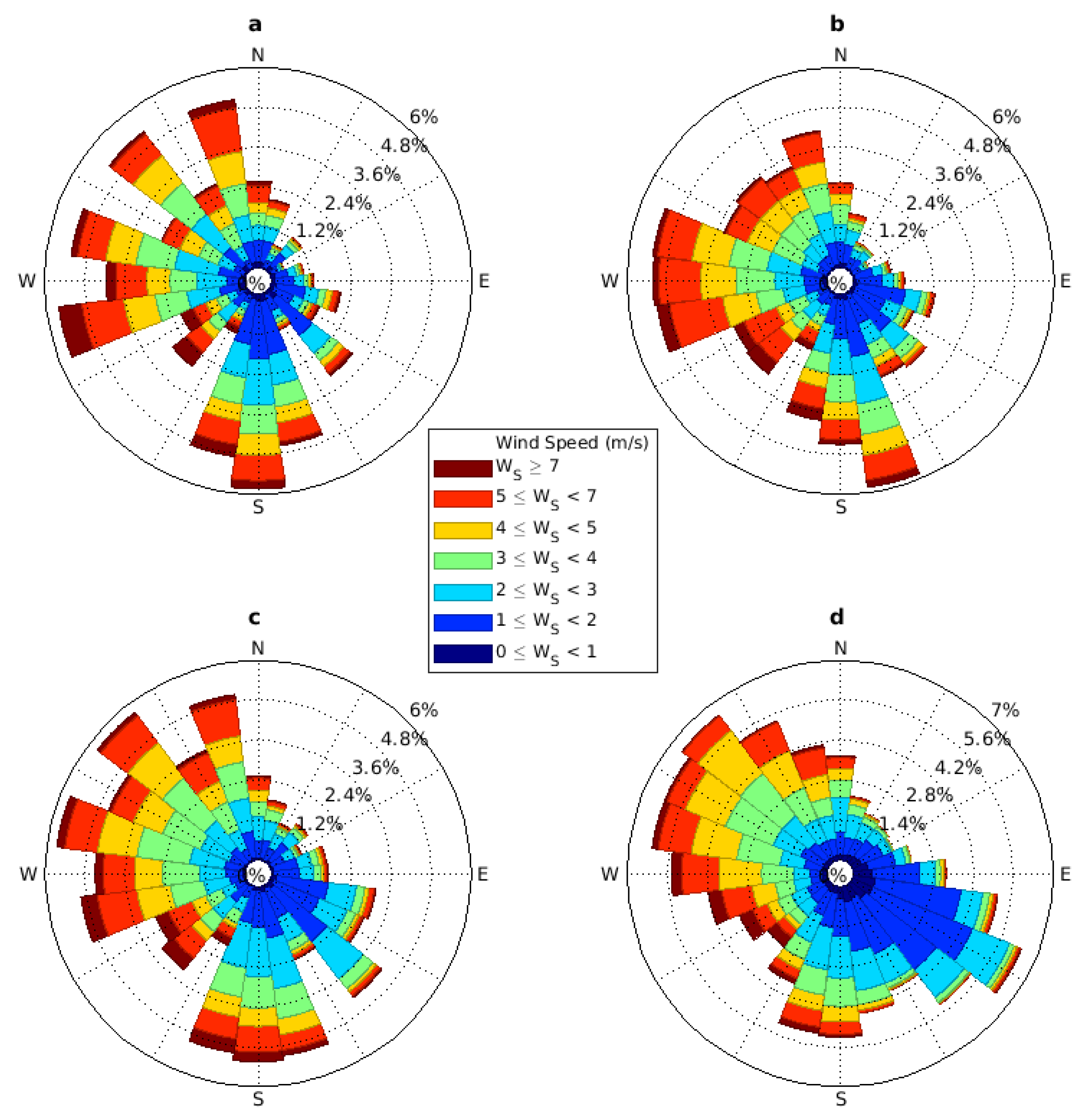
Meteorological variables were observed by many of the HBA air quality stations and by four meteorological stations operated by the Israeli Meteorological Service (IMS). For this work, only the 10-min resolution wind data (direction and speed) from the IMS Afeq station, away from the Carmel ridge and representing regional airflow patterns, were used (its location is shown in Figure S1). To get an idea about possible long-timescale changes in the typical wind patterns, we also used data from the Bet Dagan station (100 km south of HBA), which has operated since 1970. Historical Bet Dagan wind data at three h resolution were extracted for 1971–2000. The manually-operated Bet Dagan station was replaced in the early 2000s by an automatic station, reporting at a 10-min resolution. Three hour averages were extracted from the new records to continue the measures of the historic station.

2.4. Exposure Assessment: Rationale and Method

Lack of emission inventories and monitoring data for most of the study period forms a formidable hindrance in specifying the exposure to specific industry-sourced pollutants in HBA. Thus, we have decided to use a proxy variable to represent the spatial pattern of relative exposure intensities to ambient concentrations of pollutants emitted by the industrial complex to be used for the entire study period. A good candidate for such a proxy is the pattern of ambient SO2 concentrations. Several considerations justify but also somewhat constrain its use for this purpose:
(1)
Exposure to pollution from HBA industrial emissions occurs only where the emitted pollution can be transported by airflows previously passed by the industrial stacks. Thus, the industrial center location, the boundaries of residential areas, and the typical wind patterns that can bring air from the former to the latter are the most critical general considerations.
(2)
Since the late 1970s, heavy industry and, to a lesser degree, the seaport were the only substantial emitters of SO2 in HBA [29]. In recent years, with the port remaining by far its largest source, SO2 levels have been shallow and close to the monitoring analyzer’s detection and quantification limits. Thus, we assume that SO2 observations at the beginning of the 21st century, which were higher by a factor of 4–10 compared with current levels (Figure S3), were dominated by HBA heavy industry emissions. Background SO2 concentrations are not negligible [30]. Still, they can be considered in the limited aerial extent of HBA to be homogeneous without impacting the shape of the SO2 spatial patterns.
(3)
We expect SO2 dispersion and the shape of its spatial concentrations pattern to be similar to those of other industrial pollutants with comparable or a longer atmospheric lifetime.
(4)
Dispersion of industry-emitted pollutants with atmospheric lifetime shorter than that of SO2 (e.g., most VOCs) may result in different spatial patterns. Still, we expect that their dispersion lobes’ central axes will be along those of the SO2 spatial distribution (i.e., they will be contained within those of the SO2).
(5)
Use of the observed SO2 concentrations in the early years of the 21st century for assessing exposures to industrial pollution emitted in the last decades of the 20th century is warranted, only if the relevant meteorological factors (mainly the wind field) have not changed substantially. This is indeed the case in HBA (see below).
(6)
Due to the possible large decline in industry-born ambient concentrations during the study period, driven by a parallel reduction in the industrial emissions, an analysis using the spatial SO2 pattern must account for its temporal concentration variability.
(7)
SO2 spatial patterns based on relatively sparse observed concentrations (at the AQM stations) might be affected by the locations of the observations [31]. To minimize this effect, it is desirable to use as many observation sites as possible (see Figure S2). Still, reliance on small-scale details of the spatial patterns should be avoided, and only their general outline should be used.
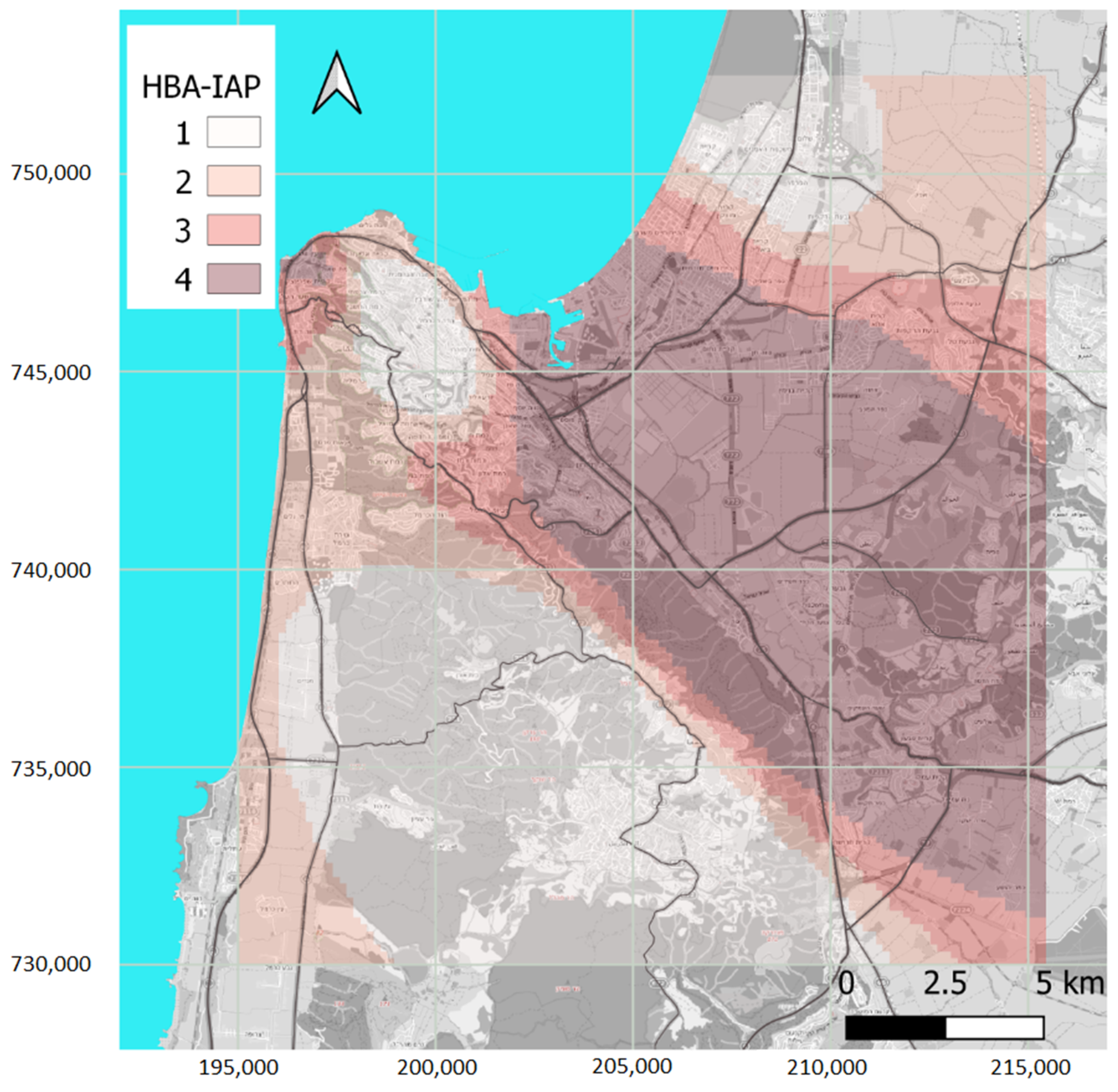
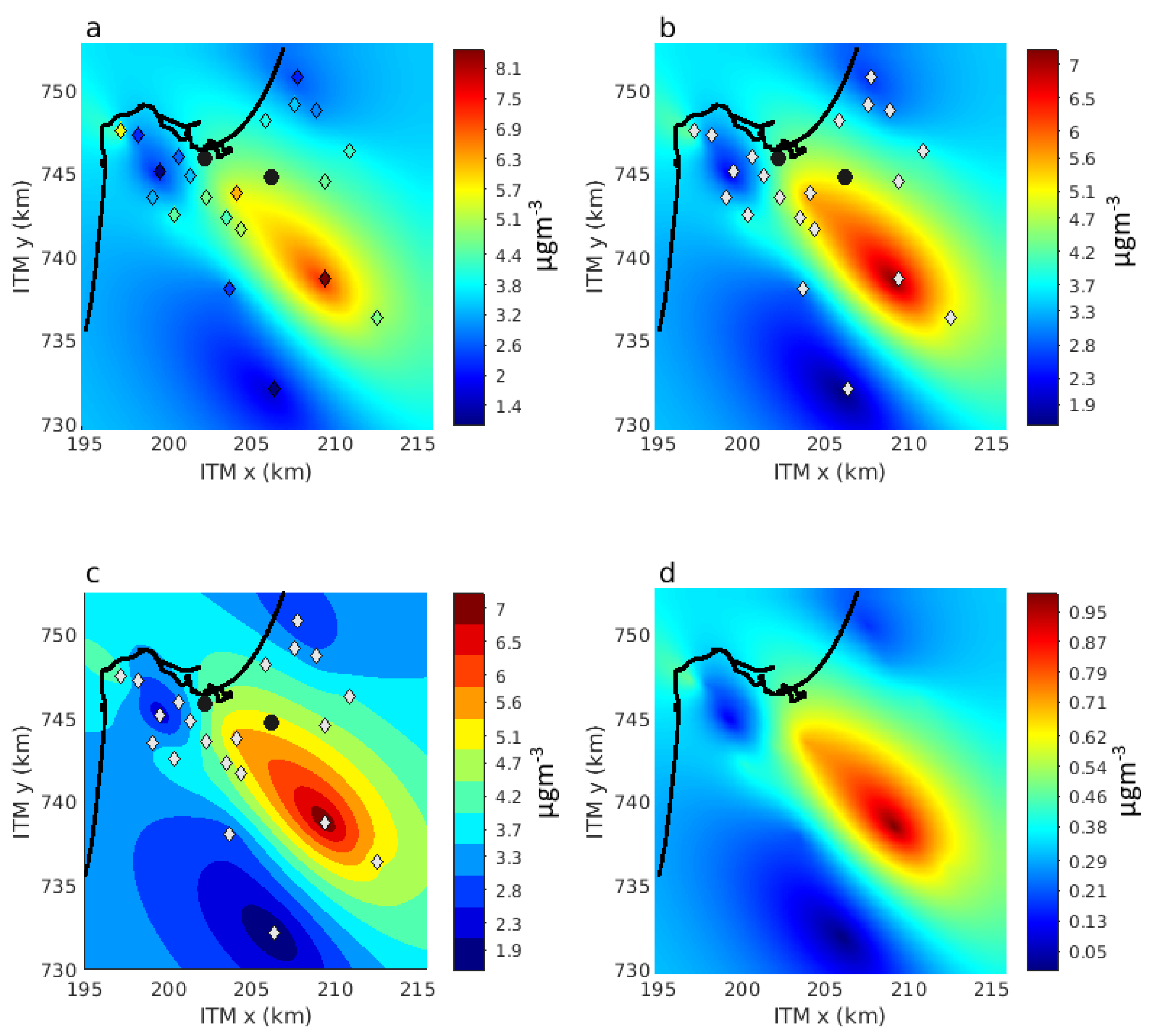
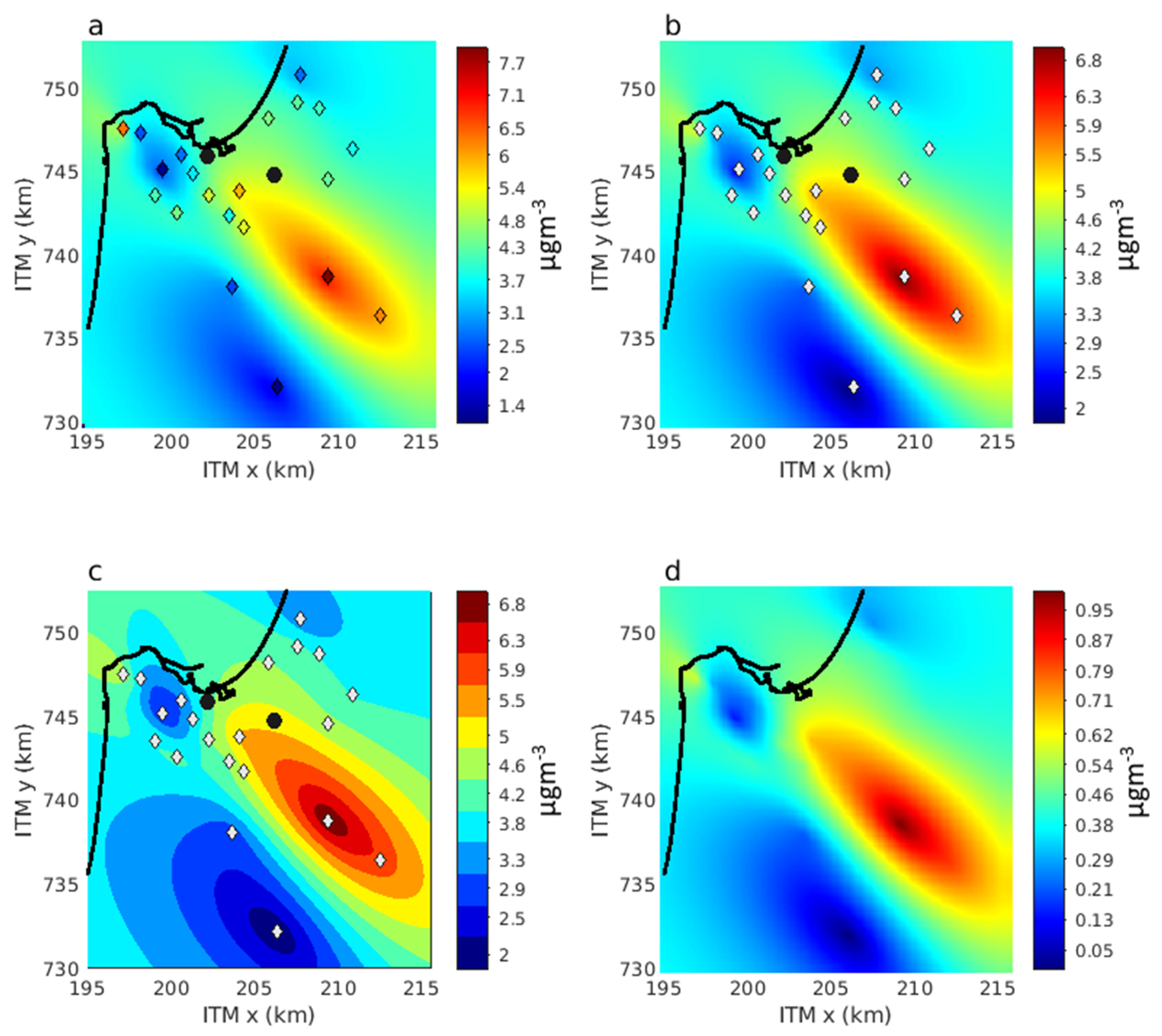
Given these considerations, we estimated the exposure to industrial emissions by a kriging interpolation of the 2002–2004 mean SO2 observations. During this period, the number of SO2 monitoring stations was maximal (Figure S2), and the ambient concentrations were still relatively high (Figure S3). The background SO2 level in this period is known [30], and a comparison to past investigation [31], which studied air pollution patterns in HBA in a similar period, is possible [17]. We used a kriging nugget effect of 1 µg/m3 to account for potential differences in the instrument calibration. We tested the sensitivity to the selected period using various combinations of years 2001–2006. We further compared the wind patterns in different periods observed in HBA by the longest-serving IMS station in the area (Afeq, Figure S1) to detect possible variability in the local wind pattern. The Afeq station’s records go back only to 2003, so we examined possible long-timescale changes in the typical winds patterns in Israel’s coastal area using data from the Bet Dagan station (100 km south of HBA) which has operated since 1970. Appendix A contains more details on the sensitivity of the SO2 spatial pattern and the long-term wind patterns.

2.5. Statistical Analyses

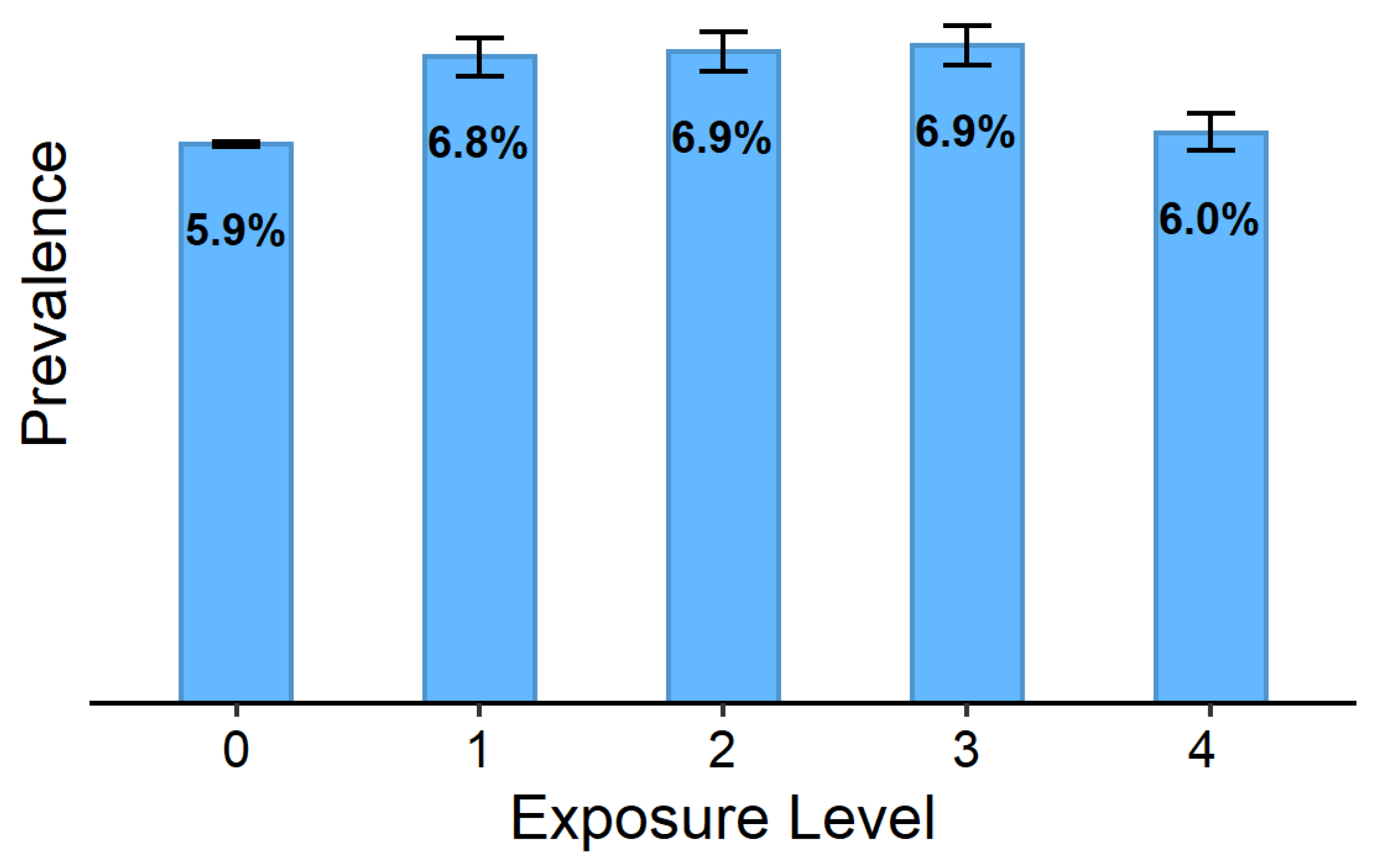
We have categorized the exposure into four time-invariant equal-participant number HBA groups and one reference group of participants who lived outside HBA, according to each subject’s residential address. Additional categorizations that we used in sensitivity analyses were of three and four equal-interval exposure groups. We calculated crude prevalence and its 95% confidence interval (CI) by exposure categories for each health outcome and presented these measures using simple bar plots and tables.
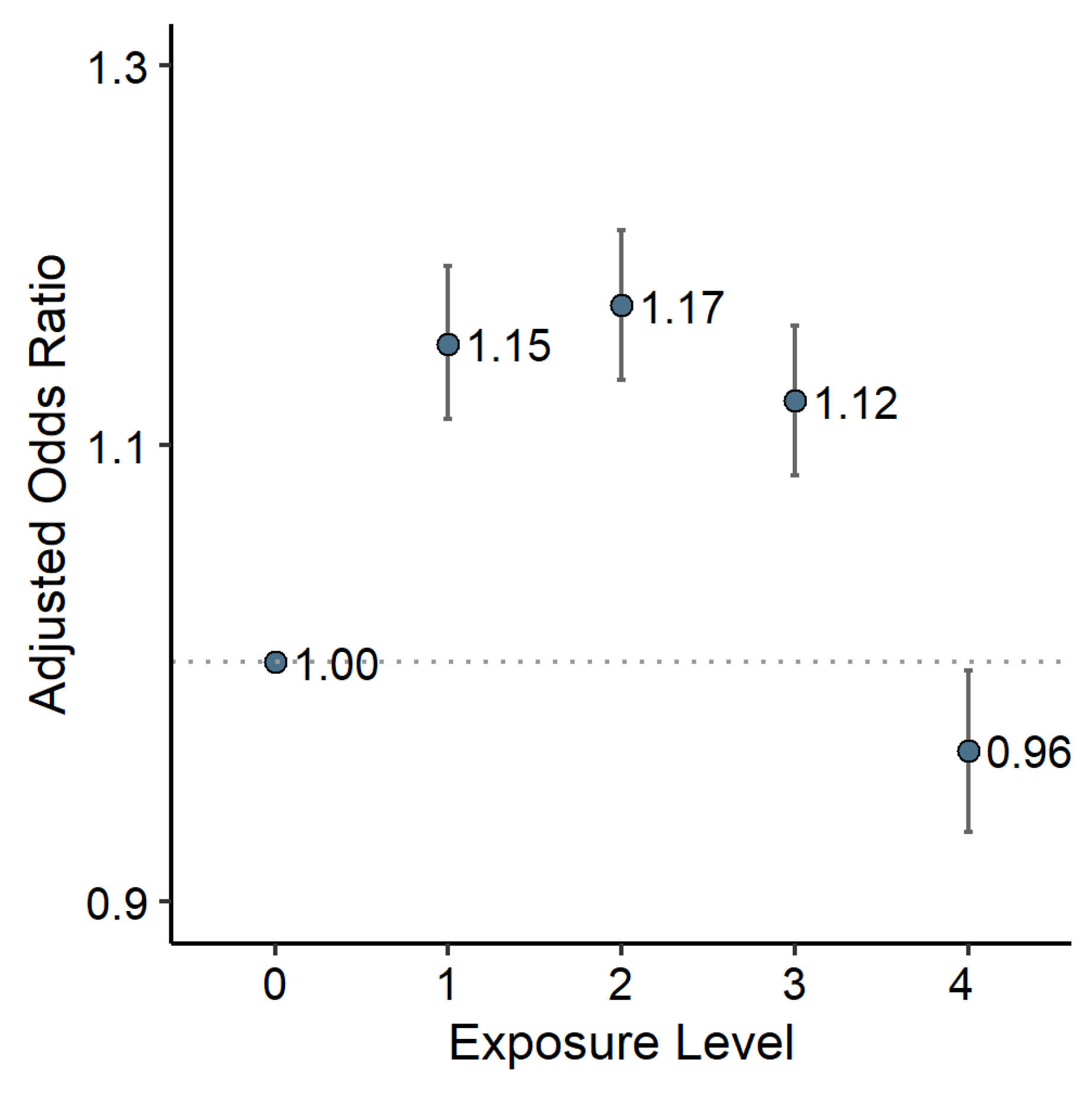
We used generalized linear models applying multivariable logistic regression analyses to examine adjusted associations between HBA industrial air pollution (HBA-IAP) and asthma or other atopic diseases. Associations were expressed as odds ratios ± 95% CI for each HBA-IAP exposure category compared with the non-HBA population that served as a reference category.
We adjusted all models for the following set of potential confounders: Year of birth, socio-economic status (SES, taken from the Central Bureau of Statistics of Israel at the level of small statistical areas), school orientation (secular, religious, or ultra-orthodox), and NOx (as a measure of traffic-related air pollution).
NOx was assessed by a land-use regression model [32,33]. This country-wide model estimates annual average NOx concentrations over Israel since 1961, with a spatial resolution of 200 m over the entire domain and 50 m in urban regions. Exposure to NOx was calculated for each adolescent from birth to age 17, based on official residential addresses around age 16. We geocoded the addresses using ArcGIS version 10.5 (ESRI, Redlands, CA, USA) and street reference data from ©HERE [34]. Furthermore, 79.8% of the addresses were geocoded with very good accuracy (full address or street level), and an additional 10.0% were geocoded at a reasonable accuracy (at the neighborhood or the locality level). Most of the remaining addresses were incomplete or contained errors that could not be corrected, and data for these adolescents were not analyzed. In HBA, where exposure assessment is critical for the current study, we were able to geocode 89.1% of the addresses with very good accuracy (full address or street level).
We further adjusted some of the models for PM2.5 concentrations, assessed by a hybrid satellite-based model [35,36]. This model estimates daily average PM2.5 concentrations over Israel since 2003 at a spatial resolution of 1 km. Since the PM2.5 model only starts from 2003, models adjusted for PM2.5 included only adolescents who were medically assessed from that year and on (approximately 35% of our study population). Exposure to PM2.5 was calculated similarly to exposure to NOx but included for each participant just the age period between birth and age 17, for which PM2.5 concentrations were available.
Stratification by decades provides an additional method to handle potential confounding by time trend except for adjustment. It is also essential since the exposure model lacks any temporal variability (i.e., HBA-IAP exposures assessed by the exposure model are constant with time per specific address). HBA-IAP has changed substantially over the total exposure period of 50 years relevant to our study population. Therefore, HBA-IAP may have been associated with a higher risk of prevalent asthma at age 17 only in some of the historical decades we examined but not in others. To investigate concerns of confounding or effect modification by period, we performed stratified models by the decade of birth.
We performed additional stratification by parental origin to partly exclude potential cultural and genetic confounders. We have defined a shortlist of countries that are commonly known as Jewish “Ashkenazi” origin (Russia and other former USSR countries, Poland, Hungary, Romania, Germany) and another list of countries that are commonly known as Jewish “Mizrahi” origin (Morocco, Iraq, Egypt, Turkey, Yemen, and Iran). In addition, we tested the effect of further adjustment for BMI and locality type (rural, urban with <50,000 residents, and urban with >50,000 residents).

3. Results

3.1. Study Population

The study population included n = 2,523,745 adolescents born in Israel between 1947 and 2001, among which 59% were males. Asthma and allergic rhinitis prevalence were 5.9% and 4.6%, respectively, while other atopic diseases were much less prevalent. Table 1 presents the study population characteristics by exposure groups, and Figure 1 shows the spatial division of the area by these categories.

3.2. Prevalence of Asthma and Other Atopic Conditions by HBA-IAP Exposure Categories

Figure 2 presents the prevalence and 95% CI of asthma, showing that this disorder’s prevalence is much higher in HBA. Still, this increased prevalence is concentrated in the three lower HBA-IAP exposure categories. In contrast, the residents who are assumed to be exposed to the highest HBA-IAP levels do not have excess asthma prevalence (for elaboration, see Supplementary Table S1).
The prevalence of rhinitis, asthma with comorbid rhinitis, atopic dermatitis, and rhinoconjunctivitis by HBA-IAP categories is presented in Figures S4–S7, respectively. HBA adolescent residents have an increased prevalence of rhinitis (with or without asthma) and rhinoconjunctivitis compared with non-HBA adolescents. However, similarly to asthma, the prevalence does not increase with increasing exposure to HBA-IAP. The highest HBA-IAP exposure group presents the lowest prevalence level within HBA, sometimes even compared to non-HBA residents (see elaboration in Supplementary Table S2).

3.3. Adjusted Associations of HBA-IAP Exposure with Prevalent Health Conditions at Age 17

The results of the primary multivariable logistic regression model of asthma, adjusted for SES, year of birth, school orientation, and NOx, are presented in Figure 3. These results show that HBA residency is associated with a higher adjusted risk of asthma (compared to the non-HBA residence). This association is limited to the three lowest HBA-IAP exposure categories. In contrast, the highest exposure group has the lowest adjusted risk.
Examination of associations between HBA-IAP and other prevalent atopic diseases at age 17: rhinitis (with or without comorbid asthma), rhinoconjunctivitis, and atopic dermatitis, showed similar exposure-response curves, where residency in HBA is associated with higher risk, except for the highest exposure group (Figure 4).

3.4. Sensitivity Analyses

All sensitivity analyses were made on the primary multivariable asthma model by either adding another variable to the adjustment set or stratifying it by another variable. Figure S8 presents an analysis with adjustment for PM2.5, which does not change the exposure-response curve substantially. An adjustment to either locality type (Figure S9) or BMI (Figure S10) also did not materially change the main models’ results.
Figure S11 shows associations between HBA-IAP exposure and asthma, stratified by four periods, based on the study population’s birth years. Despite differences in the magnitude of the associations among periods and differences in the exposure-response curves, the highest exposure category is associated with the lowest adjusted risk of asthma among all HBA groups in all periods. Stratification by parental region of origin produced, despite some differences (especially between the two lowest HBA-IAP categories within the HBA population), quite similar exposure-response curves, which are also compliant with the previous models (Figure S12).
We have also considered two additional categorizations of HBA-IAP by equal exposure intervals instead of equal-participant numbers. Table S3 and Figure S13 represent the categorization of HBA-IAP into four equal-interval exposure groups. Figures S14 and S15 display the prevalence of asthma and the adjusted associations by these categories, respectively. Table S4 and Figure S16 present the categorization of HBA-IAP into three equal interval exposure groups. Figures S17 and S18 show the prevalence of asthma and the adjusted associations by these categories, respectively. These results concur with the shape of the exposure-response curve of the main categorization, suggesting insensitivity of our analyses to the exact categorization of the exposure.

4. Discussion

This study is focused on the prevalence of asthma and other atopic diseases in adolescents at age 17 and its associations with HBA-IAP. Our results confirm that asthma prevalence is higher in Israeli-born HBA adolescents in comparison to their non-HBA counterparts. However, based on our exposure model, the association between exposure to HBA-IAP and either crude prevalence of asthma or adjusted association with the disorder is not compliant with what we expect from causal relationships. Specifically, the fact that the highest exposure group does not present higher prevalence and that this picture does not change even after adjustment for potential confounders and with various categorizations of exposure groups does not support a causal relationship between childhood exposure to HBA-IAP and prevalent asthma during adolescence. Moreover, in most models, the highest asthma prevalence was evident in the two lowest HBA-IAP categories. These results suggest that factors other than HBA-IAP may drive the higher asthma prevalence proportions in the HBA. Examinations of crude and adjusted associations of HBA-IAP with other atopic diseases show a similar picture.
Our findings have several possible explanations. Firstly, it could be that childhood exposure to HBA-IAP does not increase the risk of incident asthma during childhood or adolescence. Due to a lack of measurements, we do not have a fair characterization of the chemical and physical composition of historical emissions from the HBA industry. It is reasonable to assume that the HBA industry emitted various VOCs and particulate heavy metals. The most robust evidence in the literature about air pollution and asthma is about criteria pollutants and asthma exacerbations. The evidence about the new onset of asthma is weaker and is also limited to criteria pollutants. A lack of causal relationship between HBA-IAP and the risk of prevalent asthma in adolescence does not contradict previous epidemiological reports on the topic. It also does not imply a lack of causal relationship between HBA-IAP and asthma exacerbations.
Alternatively, we acknowledge the possibility of residual confounding that prevented us from observing the real exposure-response curve. According to this possibility, the highest HBA-IAP exposure group has a high proportion of factors that protect it from asthma than all other exposure groups. These unmeasured protective factors cannot include elements that we have adjusted for or stratified by. Therefore, it cannot result from differences among the groups, which are strongly related to time trends, SES, population group (as depicted by the school orientation variable), parents’ origin, traffic-related air pollution, or PM2.5. In addition, these protective factors must be very common in the highest exposure group and substantially impact the risk of the relevant diseases (mainly asthma).
One potential confounder for which data were unavailable to us is smoking, including environmental tobacco smoking, a strong risk factor for asthma. Smoking is also associated with factors such as SES that affect the spatial distribution of the study participants. Therefore, smoking is a potential unmeasured confounder that we could not control in our analyses, and substantially lower levels of smoking in the highly exposed population, if they exist, may account for the findings. Unfortunately, we did not have individual-level or area-level data with relevant spatial resolution on smoking. However, one should note that our study included adolescents who were examined over a range of 50 years (1967–2017). While we expect confounding by smoking to change over such an extended period, stratification by decades did not show any exposure-response curve that seems to support a causal effect in any of the periods. Besides, we did adjust our analyses for SES (at the small statistical area level) and school orientation—two variables associated with smoking prevalence in Israeli soldiers [37], thereby mitigating possible confounding by smoking. Hence, while we cannot completely rule out confounding by smoking, several arguments do not support this possibility.
Residual confounding from other factors, including genetic differences, is also possible. We partly controlled genetic factors in stratified analyses by parental origin, but we cannot completely rule them out as potential confounders. Ozone and humidity are two additional factors that we could not control for. However, these variables vary slowly in space and are not expected to have an extensive range in the study area. Therefore, they are not likely to generate confounding in this study.
Another explanation for these exposure-response curves compliant with HBA-IAP’s causal effect on prevalent asthma at age 17 is a possible interaction of this exposure with other (unmeasured) risk factors. HBA-IAP’s impact on the onset and persistence of asthma may depend on coexposure to a third factor. If this factor is not prevalent in the high exposure areas, this may explain the low prevalence of asthma and other disorders in the highly exposed population. Allergens interact with air pollutants in the causal mechanism of asthma onset. Our study does not contain individual or area-level data on exposure to allergens. Therefore, exposure to some allergens may cause the high prevalence of asthma and other atopic diseases that we have observed in the low HBA-IAP exposure groups, with or without interaction with HBA-IAP exposure. This possible mechanism may also be compliant with HBA-IAP’s causal effect on asthma’s onset and persistence if the relevant allergens are highly absent in the lowest HBA-IAP groups.
Another possible explanation of our results that may be compatible with a causal relationship is information bias due to inaccurate residential address data. We have based our exposure assessment on addresses known at the time of medical evaluation, i.e., approximately at age 16–17 and used these addresses to calculate the mean exposure from birth to age 17. Some of the adolescents, possibly many of them, changed address between birth and age 17, and none of them spent their entire life by age 17 standing outside their home. They have spent time indoors, in many other places, and probably for some of them even their home addresses were different throughout most of the period. However, one should note that as long as these exposure error components do not distribute differently among adolescents with and without the relevant health condition in the study population, we can regard this error as nondifferential (with respect to the outcome—for example, asthma). Such a nondifferential exposure error is expected, on average, to bias our associations towards the null, i.e., it is generally expected to yield associations in the same direction as the real associations but weaker. Since we did obtain strong and statistically significant associations in our study that are not compatible with a causal exposure-response curve, a nondifferential error of the exposure is unlikely to have entirely caused these results.
Nevertheless, we cannot completely disregard the possibility of differential error in our exposure assessment due to a pattern of address changes that varies by the outcome. For example, suppose families with asthmatic children who lived in the highly exposed HBA area during their child’s diagnosis are much more likely to change the address before age 16 than families of asthmatic children from other regions. In that case, this would bias our crude and adjusted associations, which are based solely on prevalent asthma at age 17 and addresses around that age. Naturally, most of the addresses in the highest HBA-IAP exposure category are surrounding the industrial area or are downwind of it. Parents of children diagnosed with asthma in this region may have thought it would be better for their child to live in another area and consequently moved to a different location before age 17. In our analyses, such children cases would have been counted in their new addresses and would have reduced the observed prevalence of asthma at age 17 in the areas from which they moved, e.g., the high HBA-IAP exposure group. Moreover, if these families moved to less exposed HBA areas, they increased asthma prevalence at age 17 in these areas. If such bias exists, it may explain our results and be compatible with HBA-IAP’s causal effect on asthma onset. Unfortunately, we did not have data on addresses other than around age 17, so we could not assess likelihood of this bias.
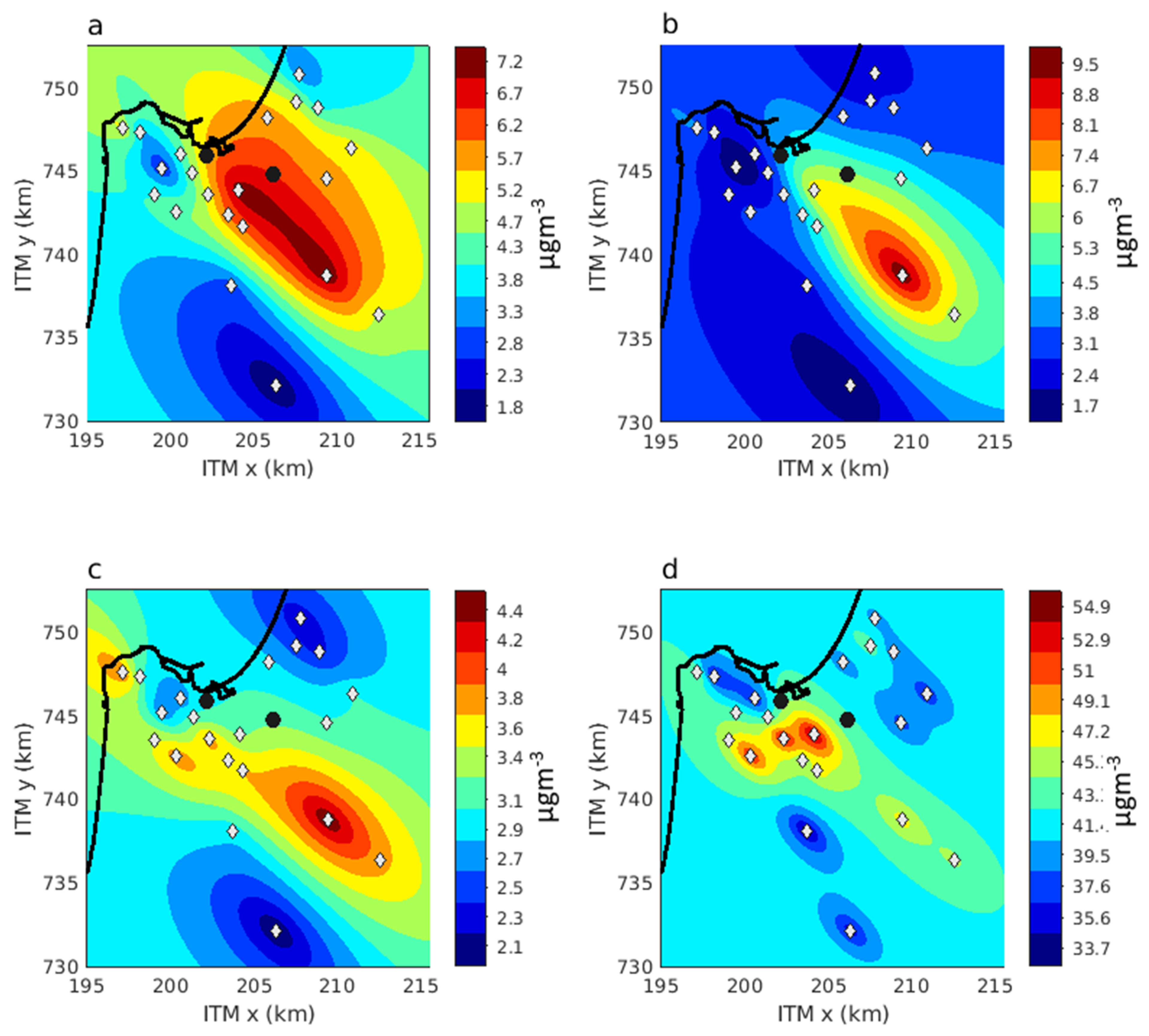
Another possible explanation of our results which may have some compliance with a causal relationship is that the exposure that matters for a causal effect is not the average exposure. For example, exposure to HBA-IAP varies by the time of the day. It is determined mostly by meteorological factors such as the wind field (speed and wind direction) and atmospheric stability. Specifically, the spatial distribution of HBA-IAP during the night is different from that during the day (Figure A1). The concentrations of inhaled pollutants and the presence of children and adolescents indoors also vary by the hour of the day. We did not consider these factors in our epidemiological models, but some combination of these factors may be biasing our results. These issues require careful characterization and may be explored in future studies.
The main limitation of this study is its cross-sectional design, which limits causal inference. This design resulted from the nature of the dataset we used, in which only one address and only one medical evaluation were available per participant, both around age 17. Ideally, one would need data on addresses from birth to diagnosis or end of follow-up and relevant diagnosis date to make a much more robust inference on the causal relationship between exposure to pollution and risk of the onset of new asthma. However, such data were not available to us. On the other hand, the current dataset is unique because it is based on mandatory medical screening. It also includes a comprehensive country-wide population-based sample that spans over 50 years of exposure and outcome data.
Another limitation is our exposure data, which is not ideal for an epidemiological study. We have made a substantial effort to classify our study population by exposure to HBA-IAP. However, this exposure assessment lacks temporal variability, characterization of the relevant pollutants, and direct measures of these pollutants—components that would have improved it had they been available. Prior studies characterized HBA exposure on either distance from the industrial area, measurement of criteria pollutants, or merely comparing HBA to non-HBA residents [15,16,17,18,20]. We have used a new approach to categorize the HBA population by levels of exposure to HBA-IAP, and think that this approach is better than the other available assessment method of historical HBA-IAP unmeasured pollutants.
Our lack of data on addresses before age 17, and lack of data about school addresses, which may account for a substantial portion of the exposure [38], are additional limitations of this study. We have limited our sample to Israeli-born adolescents to mitigate this problem, but we acknowledge that this is one of our main limitations. However, epidemiological theory can predict the bias created by such inaccuracy of exposure data and the rare circumstances under which a real causal relationship is hidden in our results, as discussed above for differential error of address change. Our study is also limited by the outcomes we have examined. The most important limitation in this context is that we used prevalent health conditions without considering disease onset, clinical disease course, exacerbation, and other clinical characteristics. In addition, our findings cannot be generalized to asthma in adults.
Finally, we need to acknowledge our inability to better adjust for potential confounders, especially for smoking. We have made efforts to examine possible residual confounding by various stratification methods, different categorization methods of the exposure, and adjustment for proxies in this context. The fact that these additional analyses did not materially change the exposure-response curve renders the possibility that our main findings are solely a result of residual confounding less likely.

5. Conclusions

The analyses we performed do not support causal relationships between exposure to HBA industry-related emissions of ambient pollutants and prevalent asthma or other atopic diseases at age 17.

Supplementary Materials

All supplementary figures and tables are available online at https://www.mdpi.com/article/10.3390/atmos12040516/s1. Figure S1: Study area map. Superimposed on the HBA elevation map are the shoreline (blue.continuous line), locations of the industrial stack from the 2015 Ministry of Environmental Protection report (red circles), the site of the historical Nesher cement plant furnace (black circle), the location of the Afeq meteorological station (yellow square), and the loca-tions and numbers of the SO2 air quality monitoring stations whose data were used (green diamonds). The coordinates are in the New Israel Mercator projection (in km). Figure S2: The number of air quality monitoring stations that observed SO2 in HBA at each of 1991-2016. Figure S3: Annual means of SO2 concentrations in a sample of five air quality monitoring stations in HBA. The station number corresponds to the numbers in Figure S1. Figure S4: Crude prevalence of rhinitis by HBA-IAP categories. 0 = reference category (non-HBA residents), 1= lowest HBA-IAP exposure. Figure S5: Crude prevalence of asthma with comorbid rhinitis by HBA-IAP categories. 0 = reference category (non-HBA residents), 1 = lowest HBA-IAP exposure. Figure S6: Crude prevalence of atopic dermatitis by HBA-IAP categories. 0 = reference category (non-HBA residents), 1 = lowest HBA-IAP exposure. Figure S7: Crude prevalence of rhinoconjunctivitis by HBA-IAP categories. 0= reference category (non-HBA residents), 1 = lowest HBA-IAP exposure. Figure S8: Association between HBA-IAP and asthma, adjusted for SES, year of birth, school orientation, NOx, and PM2.5. N = 791,132, N = 57,573. 0 = reference category (non-HBA residents), 1= lowest HBA-IAP exposure. Figure S9: Association between HBA-IAP and asthma, adjusted for SES, year of birth, school orientation, NOx, and lo-cality type. N = 2,294,152, N cases = 139,400. 0= reference category (non-HBA residents), 1= lowest HBA-IAP exposure. Figure S10: Association between HBA-IAP and asthma, adjusted for SES, year of birth, school orientation, NOx, and BMI category. N = 2,248,006, N cases = 139,419. 0= reference category (non-HBA residents), 1= lowest HBA-IAP expo-sure. Figure S11: Association between HBA-IAP and asthma, stratified by the decade of birth and adjusted for SES, year of birth, school orientation, and NOx. 0 = reference category (non-HBA residents), 1 = lowest HBA-IAP exposure category. Figure S12: Association between HBA-IAP and asthma, stratified by parental region of birth and adjusted for SES, year of birth, and school orientation. A- both parents from Jewish "Ashkenazi" country (N = 147,121); B- one parent from Jewish “Ashkenazi” country and the other one Israeli-born (N = 61,636); C- one parent from Jewish “Ashkenazi” country and the other one from Jewish "Mizrahi" country (N = 86,759); D- both parents from Jewish "Mizrahi" country (N = 321,001); E- one parent from Jewish “Mizrahi” country and the other one Israeli-born (N = 79,002); F- all other partici-pants (N = 1,828,226). 0 = reference category (non-HBA residents), 1 = lowest HBA-IAP exposure. Figure S13: A map of the HBA-IAP exposure model with equal-interval color-coded exposure categories 1–4. Figure S14: Crude prevalence of Asthma by HBA-IAP four equal-interval categories. 0 = reference category (non-HBA residents), 1 = lowest HBA-IAP exposure. Figure S15: Association between HBA-IAP and asthma with four equal-interval categories, adjusted for SES, year of birth, and school orientation. 0= reference category (non-HBA residents), 1 = lowest HBA-IAP exposure. Figure S16: A map of the HBA-IAP exposure model with equal-interval color-coded exposure categories 1–3. Figure S17: Crude prevalence of Asthma by HBA-IAP three equal-interval categories. 0 = reference category (non-HBA residents), 1 = lowest HBA-IAP exposure. Figure S18: Association between HBA-IAP and asthma with three equal-interval categories, adjusted for SES, year of birth, and school orientation. 0 = reference category (non-HBA residents), 1 = lowest HBA-IAP exposure. Table S1: Distribution of subjects by exposure to HBA-IAP and asthma. Table S2: Distribution of subjects by exposure to HBA-IAP and additional atopic conditions. Table S3: Equal-interval HBA-IAP exposure (four groups). Table S4: Equal-interval HBA-IAP exposure (three groups).

Author Contributions

Conceptualization, J.D.K., R.R., G.T., Y., L.K.-B., N.L. and D.M.B.; methodology, J.D.K., R.R., R.H.-K., Y. and N.L.; validation, R.L.B.-O., D.T., R.H.-K., E.D. and R.R.; formal analysis, R.R. and R.L.B.-O.; resources, R.R., A.L., N.L. and A.A.; data curation, R.R., R.L.B.-O. and G.T.; investigation, R.R., R.L.B.-O., G.T.; writing—original draft preparation, R.R.; writing—review and editing, D.M.B., Y., A.G.-H., L.K.-B., L.B., A.A., N.L., E.D. and G.T.; visualization, R.R., Y. and R.L.B.-O.; supervision, R.R. and G.T.; project administration, R.R., A.A., G.T., L.K.-B. and R.S.; funding acquisition, J.D.K., R.R. and L.K.-B. All authors have read and agreed to the published version of the manuscript.

Funding

The Israel Ministry of Environmental Protection funded this research, grant number 161-2-9.

Institutional Review Board Statement

The study was conducted according to the guidelines of the Declaration of Helsinki, and approved by the Institutional Review Board of Medical Corps of the Israel Defense Forces (protocol 1663-2011; Initially approved on October 6 2011 and in its amended to version on March 13 2019).

Informed Consent Statement

Patient consent was waived due to de-identification and lack of practical way to achieve consent.

Data Availability Statement

Access to the health data in this study is restricted by the medical corps for privacy reasons and cannot be made public.

Acknowledgments

We wish to thank Yael Dubowski, Hadas Magen-Molho, Ruthie Harari-Kremer, Itai Kloog, Raeed Kayouf, Isabella Karakis, Orna Matzner, and Ilan Levi for their help with providing data, review, comments, or other forms of service in this project. We dedicate this article to our colleague and mentor, Jeremy D. Kark, who passed away before completing this work. Jeremy was a pioneer in epidemiology in Israel who initiated the medical corps database usage for epidemiological studies and was the principal investigator of this study.

Conflicts of Interest

The authors declare no conflict of interest. The funders had no role in the study’s design, in the collection, analyses, or interpretation of data, in the writing of the manuscript, or in the decision to publish the results.

Appendix A

Appendix A.1. The Sensitivity of the SO2 Spatial Pattern

We have based the exposure estimate in the study on kriging interpolation of 2001–2004 mean SO2 concentrations in 21 air quality monitoring (AQM) stations in HBA. Figure A1 shows the SO2 interpolation map. In Figure A1a, we present the map as continuously varying concentrations on which we superimposed the observed values. We adjusted the color-coding to the range of values of the observations, which due to the use of the nonzero nugget effect, is wider than the range found in the interpolation map. Figure A1b shows the same map but with the concentration color-coding adjusted to the range of values in the map. Figure A1c shows the interpolation map with its values assigned into 12 discrete concentration ranges. Such a map visualization is better for the determination of the exposure cutoff values among exposure categories. Figure A1d is similar to Figure A1b but with the concentration values mapped into the (0–1) range. This mapping conserves the spatial features while the map values are independent of the actual concentration range. It enables comparing spatial features in maps with different concentration ranges. For example, as a sensitivity test additional set of SO2 kriging maps is shown in Figure A2, which corresponds to the set in Figure A1 but is based on data from 2001 to 2006, the full period in which the SO2 monitoring array had its maximal value of 21 AQM stations. The range of values in Figure A1 and Figure A2 is different, but a comparison of their features, not biased by the color-coding schemes, can be made using the maps in Figure A1d and Figure A2d. The differences are minor, attesting to the weak sensitivity of the SO2 spatial feature to the choice of data period used to create it.
Figure A1. Kriging map of SO2 concentrations in the study area using data from 2002 to 2004. The black circles denote the power plant’s geographical centers and the refineries compound (west and east, respectively). (a) Continuous color-coded concentration map with the observed concentrations shown in their monitoring locations. The color-coding is tailored to the concentrations of the map and the observations. (b) Continuous color-coded concentration map with color-coding tailored to the map values. (c) The same as (b) but with the map values assigned to 12 concentrations ranges. (d) The same as (b) but the concentrations values mapped into the (0–1) range.
Atmosphere 12 00516 g0a1
Figure A2. Similar to Figure A1, but using data from 2001 to 2006. (a) Continuous color-coded concentration map with the observed concentrations shown in their monitoring locations. The color-coding is tailored to the concentrations of the map and the observations. (b) Continuous color-coded concentration map with color-coding tailored to the map values. (c) The same as (b) but with the map values assigned to 12 concentrations ranges. (d) The same as (b) but the concentrations values mapped into the (0–1) range.
Atmosphere 12 00516 g0a2
Figure A1 and Figure A2’s main concentration features are similar to those in the SO2 concentration map shown in Figure 8 in Yuval and Broday (2006) [31]. That figure was produced by the optimized interpolation scheme of Yuval et al. (2005) [39] using data from AQM stations 1–20 (i.e., one station less than here) and interpolating over a smaller spatial extent. The main difference is in the concentration range, which in the current work is narrower due to the more relaxed fitting of the interpolation to the observations through using nugget value of 1 µg/m3 vs. zero nugget in Yuval and Broday (2006) [31]. We carried out similar sensitivity tests using data from different combinations of years from 2001 to 2006. We found weak sensitivity of the SO2 spatial feature to the choice of data years used.
We illustrate a set of different sensitivity is in Figure A3. It shows some alternatives to the map in Figure A1b, the one selected for representing the risk due to industrial borne pollutants. Figure A3a–c show the kriging interpolation of SO2 concentrations from 2002 to 2004 observed during three periods of the day. The shapes of the spatial SO2 concentration patterns and the associated concentration ranges are quite different from one another and from the spatial pattern in Figure A1b. People’s potential to be exposed to industrial emissions varies throughout the day, depending on being indoors or outdoors, indoor ventilation efficiency, outdoor physical activity, and so on. Therefore, the different SO2 concentration patterns shown in Figure A3a–c might mean that the impact of industrial pollution is not necessarily optimally reflected by Figure A1b.
Figure A3d shows the kriging interpolation of SO2 concentration from 2002 to 2004 but considering only concentrations above 20 µg/m3. The spatial pattern that it offers is different from the corresponding one in Figure A1b, which used the full range’s concentration values. In case the impact of HBA-IAP has some threshold effect, the hot exposure spots in Figure A3d might be a better metric to study the possible effect of industrial pollution than the pattern resulting from using observations of the full range of values. While this may be suitable for allergens, it is probably not relevant for mutagens, which may be carcinogenic and assumed to have no safe threshold concentrations.
Figure A3. Kriging map of SO2 concentrations in the study area using data from 2002 to 2004. The black circles denote the power plant’s geographical centers and the refineries compound (west and east, respectively). (a) Using only observations between 06:00 and 13:30. (b) Using only observations between 14:00 and 21:30. (c) Using only observations between 22:00 and 05:30. (d) Using only observations from 20 µg/m3 and up (all hours of the day).
Atmosphere 12 00516 g0a3

Appendix A.2. Temporal Variability of the Wind Pattern

Figure A1 and Figure A2 reflect the SO2 dispersion at the beginning of the 21st century. To test their relevance for exposure to HBA industrial pollution since the 1950s (when the earlier study participants were born), we should examine the meteorological variables affecting the dispersion in the last few decades. The most important meteorological factors affecting the dispersion of emissions from the HBA industrial center are the wind speed and direction. Characteristics of atmospheric stability and stratification can also play a role in the dilution of emissions. Unfortunately, reliable high-resolution vertical profiles of temperature, barometric pressure, and vapor content are available only from radiosonde launches in the Bet Dagan meteorological station in central Israel. Bet Dagan’s terrain is flat, so the planetary boundary layer there might not represent well that in HBA, where the topography includes very steep slopes (Figure S1). Given that the high-resolution Bet Dagan radiosonde records start from 2007, we did not carry out an analysis of the temporal trends of the atmospheric stability and stratification.
The prevailing wind is the meteorological variable that mostly affects the spatial pattern of the HBA industry’s pollutants. The wind direction determines the central axis of the dispersion plume. The wind speed is one of the variables that determine the dilution rate and the intensity of the pollution concentrations along and around the center of the plume. Changes in the wind patterns may thus impact the dispersion of the pollutant and their spatial distribution. Figure A4 shows the wind roses of the wind observed in the Israeli Meteorological Service (IMS) Afeq station (Figure S1 in the main article) in four different periods. Afeq is the only IMS station in HBA away from the Carmel mountain, and therefore the measured wind patterns should reflect the general flow pattern in the area. Due to the Carmel mountain’s very steep topography (Figure S1), the wind observed on it changes significantly even between locations at close geographical proximity.
The four wind roses in Figure A4 are not identical, but they all show very similar wind patterns. The most frequent are relatively strong winds from the northwest. Such winds carry pollution emitted by the industrial stacks shown in Figure S1 to the southeast and result in the main lobe of high SO2 concentrations shown in Figure A1 and Figure A2. The second most prominent pattern is of winds from the south and southeast directions, which are mostly weak and include some of the strongest ones. Wind from the south can carry pollution emitted in the refineries compound (the eastern group of stacks) towards AQM stations 1–4. Southeasterly wind can carry pollution emitted from all the industrial stacks towards the Carmel mountain and Haifa. The above is a very simplistic description, and the actual flow patterns must be very complicated. However, looking at Figure A4, it seems that in the last 20 years or so, the wind patterns have probably not changed much, so the SO2 spatial patterns shown in Figure A1 and Figure A2 should represent industrial pollution patterns in the 21st century well.
Figure A4. Wind roses of wind observed in the Afeq station in the years (a) 2003–2006; (b) 2007–2010; (c) 2011–2014; (d) 2015–2016.
Atmosphere 12 00516 g0a4
None of the meteorological stations in HBA operated before 2000. Thus, to study possible wind pattern changes since the 1970s wind data from the IMS Bet Dagan station were used. A similar wind regime prevails all along the Israeli coast, so to examine long trends in the wind patterns, the Bet Dagan wind records can serve as a proxy to the general airflow in HBA. Until the early 2000s, the Bet Dagan observations were manually-operated at a three h temporal resolution, and only since then the station operates automatically and reports at 10 min resolution. Figure A5 shows wind roses created using the Bet Dagan wind data in four decades, starting in the 1970s. The wind rose for 2000–2009 looks different from the ones for previous decades. It is very similar though to that for 2010–2016 (not shown). The change since 2000 is most probably due to the switch from the old manually operated station to the automatic one. The three wind roses for the 1970s, 1980s, and 1990s are not identical, but they demonstrate very similar features, with the most common winds from the southwest to northwest and the south directions.
Figure A5. Wind roses of wind observed in the Bet Dagan meteorological station in the years (a) 1970–1979; (b) 1980–1989; (c) 1990–1999; (d) 2000–2009.
Atmosphere 12 00516 g0a5
Formal ways to quantitatively compare wind roses exist (e.g., Walmsley and Bagg, 1978) [40] but were not applied here. Given the many possible changes in measurement procedures and data errors that might have occurred in the days of manual wind observations, a quantitative comparison of the historical wind data might reflect these issues more than actual climatic changes. Based on visual inspection of the wind roses, it seems that real changes might have occurred but that the principal axes of the wind in Bet Dagan, and thus most probably in HBA too, remained the same. The dispersion of pollutants in HBA probably has not undergone, on average, very significant changes. Therefore, the SO2 spatial pattern based on the early 2000s should roughly reflect the pattern of pollution dispersion in previous times.

References

  1. Goren, A.I.; Hellman, S.; Brenner, S.; Egoz, N.; Rishpon, S. Prevalence of respiratory conditions among schoolchildren exposed to different levels of air pollutants in the Haifa Bay Area, Israel. Environ. Health Perspect. 1990, 89, 225–231. [Google Scholar] [CrossRef]
  2. Tritscher, T.; Raz, R.; Levi, Y.; Levy, I.; Broday, D.M. Emissions vs. turbulence and atmospheric stability: A study of their relative importance in determining air pollutant concentrations. Sci. Total Environ. 2020, 733, 139300. [Google Scholar] [CrossRef]
  3. Israel Ministry of Environmental Protection. Air Quality Data. Available online: https://www.svivaaqm.net/Default.rtl.aspx (accessed on 31 August 2020).
  4. Wolf, K.; Cyrys, J.; Harciníková, T.; Gu, J.; Kusch, T.; Hampel, R.; Schneider, A.; Peters, A. Land use regression modeling of ultrafine particles, ozone, nitrogen oxides and markers of particulate matter pollution in Augsburg, Germany. Sci. Total Environ. 2017, 579, 1531–1540. [Google Scholar] [CrossRef] [Green Version]
  5. Irigaray, P.; Newby, J.A.; Clapp, R.; Hardell, L.; Howard, V.; Montagnier, L.; Epstein, S.; Belpomme, D. Lifestyle-related factors and environmental agents causing cancer: An overview. Biomed. Pharmacother. 2007, 61, 640–658. [Google Scholar] [CrossRef] [PubMed]
  6. Rumchev, K.; Brown, H.; Spickett, J. Volatile organic compounds: Do they present a risk to our health? Rev. Environ. Health 2007, 22, 39–55. [Google Scholar] [CrossRef] [PubMed]
  7. Maio, S.; Simoni, M.; Baldacci, S.; Sherrill, D.; Viegi, G. Indoor air pollution and airway disease. Int. J. Tuberc. Lung Dis. 2004, 8, 1401–1415. [Google Scholar]
  8. Miller, R.L.; Peden, D.B. Environmental effects on immune responses in patients with atopy and asthma. J. Allergy Clin. Immunol. 2014, 134, 1001–1008. [Google Scholar] [CrossRef] [PubMed] [Green Version]
  9. Weisel, C.P. Assessing exposure to air toxics relative to asthma. Environ. Health Perspect. 2002, 110 (Suppl. 4), 527–537. [Google Scholar] [CrossRef] [PubMed] [Green Version]
  10. Delfino, R.J. Epidemiologic evidence for asthma and exposure to air toxics: Linkages between occupational, indoor, and community air pollution research. Environ. Health Perspect. 2002, 110 (Suppl. 4), 573–589. [Google Scholar] [CrossRef] [PubMed]
  11. Health Status in Israel 2010. Israeli Center for Disease Control (ICDC). 2011. Available online: https://www.health.gov.il/PublicationsFiles/Health_Status_in_Israel2010.pdf (accessed on 5 March 2021).
  12. Jan, A.T.; Azam, M.; Siddiqui, K.; Ali, A.; Choi, I.; Haq, Q.M.R. Heavy metals and human health: Mechanistic insight into toxicity and counter defense system of antioxidants. Int. J. Mol. Sci. 2015, 16, 29592–29630. [Google Scholar] [CrossRef] [Green Version]
  13. Rosa, M.J.; Benedetti, C.; Peli, M.; Donna, F.; Nazzaro, M.; Fedrighi, C.; Zoni, S.; Marcon, A.; Zimmerman, N.; Wright, R.; et al. Association between personal exposure to ambient metals and respiratory disease in Italian adolescents: A cross-sectional study. BMC Pulm. Med. 2016, 16, 6. [Google Scholar] [CrossRef] [PubMed] [Green Version]
  14. Dunea, D.; Iordache, S.; Liu, H.-Y.; Bøhler, T.; Pohoata, A.; Radulescu, C. Quantifying the impact of PM2.5 and associated heavy metals on respiratory health of children near metallurgical facilities. Environ. Sci. Pollut. Res. 2016, 23, 15395–15406. [Google Scholar] [CrossRef] [PubMed] [Green Version]
  15. Paz, S.; Linn, S.; Portnov, B.A.; Lazimi, A.; Futerman, B.; Barchana, M. Non-Hodgkin Lymphoma (NHL) linkage with residence near heavy roads—A case study from Haifa Bay, Israel. Health Place 2009, 15, 636–641. [Google Scholar] [CrossRef] [PubMed]
  16. Zusman, M.; Dubnov, J.; Barchana, M.; Portnov, B.A. Residential proximity to petroleum storage tanks and associated cancer risks: Double Kernel Density approach vs. zonal estimates. Sci. Total Environ. 2012, 441, 265–276. [Google Scholar] [CrossRef]
  17. Eitan, O.; Barchana, M.; Dubnov, J.; Linn, S.; Carmel, Y.; Broday, D.M. Spatial analysis of air pollution and cancer incidence rates in Haifa Bay, Israel. Sci. Total Environ. 2010, 408, 4429–4439. [Google Scholar] [CrossRef]
  18. Portnov, B.A.; Dubnov, J.; Barchana, M. Studying the association between air pollution and lung cancer incidence in a large metropolitan area using a kernel density function. Socioecon. Plann. Sci. 2009, 43, 141–150. [Google Scholar] [CrossRef]
  19. Svechkina, A.; Portnov, B.A. A new approach to spatial identification of potential health hazards associated with childhood asthma. Sci. Total Environ. 2017, 595, 413–424. [Google Scholar] [CrossRef]
  20. Rottenberg, Y.; Zick, A.; Barchana, M.; Peretz, T. Organ specific cancer incidence in an industrial sub-district: A population-based study with 12 years follow up. Am. J. Cancer Epidemiol. Prev. 2013, 1, 13–22. [Google Scholar]
  21. Freedman, D. The Ecological Fallacy. Available online: http://www.stat.berkeley.edu/~census/ecofall.txt (accessed on 5 March 2021).
  22. Twig, G.; Yaniv, G.; Levine, H.; Leiba, A.; Goldberger, N.; Derazne, E.; Shor, D.B.A.; Tzur, D.; Afek, A.; Shamiss, A.; et al. Body-mass index in 2.3 million adolescents and cardiovascular death in adulthood. N. Engl. J. Med. 2016, 374, 2430–2440. [Google Scholar] [CrossRef]
  23. Twig, G.; Reichman, B.; Afek, A.; Derazne, E.; Hamiel, U.; Furer, A.; Gershovitz, L.; Bader, T.; Cukierman-Yaffe, T.; Kark, J.D.; et al. Severe obesity and cardio-metabolic comorbidities: A nationwide study of 2.8 million adolescents. Int. J. Obes. 2019, 43, 1391–1399. [Google Scholar] [CrossRef]
  24. Furer, A.; Afek, A.; Sommer, A.; Keinan-Boker, L.; Derazne, E.; Levi, Z.; Tzur, D.; Tiosano, S.; Shina, A.; Glick, Y.; et al. Adolescent obesity and midlife cancer risk: A population-based cohort study of 2·3 million adolescents in Israel. Lancet Diabetes Endocrinol. 2020, 8, 216–225. [Google Scholar] [CrossRef]
  25. Twig, G.; Zucker, I.; Afek, A.; Cukierman-Yaffe, T.; Bendor, C.D.; Derazne, E.; Lutski, M.; Shohat, T.; Mosenzon, O.; Tzur, D.; et al. Adolescent Obesity and Early-Onset Type 2 Diabetes. Diabetes Care 2020, 43, 1487–1495. [Google Scholar] [CrossRef] [PubMed]
  26. Leiba, A.; Fishman, B.; Twig, G.; Gilad, D.; Derazne, E.; Shamiss, A.; Shohat, T.; Ron, O.; Grossman, E. Association of Adolescent Hypertension with Future End-stage Renal Disease. JAMA Intern. Med. 2019, 179, 517–523. [Google Scholar] [CrossRef]
  27. Leiba, A.; Twig, G.; Vivante, A.; Skorecki, K.; Golan, E.; Derazne, E.; Tzur, D.; Grossman, E.; Dichtiar, R.; Kark, J.D.; et al. Prehypertension among 2.19 million adolescents and future risk for end-stage renal disease. J. Hypertens. 2017, 35, 1290–1296. [Google Scholar] [CrossRef]
  28. Galili, E.; Barzilai, A.; Twig, G.; Caspi, T.; Daniely, D.; Shreberk-Hassidim, R.; Astman, N. Allergic rhinitis and asthma among adolescents with psoriasis: A population-based cross-sectional study. Acta Derm. Venereol. 2020, 100, 1–5. [Google Scholar] [CrossRef] [PubMed]
  29. Operating Cars (Engine and Fuel) (Diesel for Transportation) Statute; Israel. 2003. Available online: https://www.nevo.co.il/law_html/law01/999_952.htm (accessed on 5 March 2021).
  30. Asaf, D.; Pedersen, D.; Peleg, M.; Matveev, V.; Luria, M. Evaluation of background levels of air pollutants over Israel. Atmos. Environ. 2008, 42, 8453–8463. [Google Scholar] [CrossRef]
  31. Broday, D.M. High-resolution spatial patterns of long-term mean concentrations of air pollutants in Haifa Bay area. Atmos. Environ. 2006, 40, 3653–3664. [Google Scholar] [CrossRef]
  32. Levy, I.; Levin, N.; Yuval, Y.; Schwartz, J.D.; Kark, J.D. Back-extrapolating a land use regression model for estimating past exposures to traffic-related air pollution. Environ. Sci. Technol. 2015, 49, 3603–3610. [Google Scholar] [CrossRef] [PubMed] [Green Version]
  33. Levy, I.; Broday, D.M. Improving modeled air pollution concentration maps by residual interpolation. Sci. Total Environ. 2017, 598, 780–788. [Google Scholar] [CrossRef]
  34. Real Time Maps & Map Data|HERE. Available online: https://www.here.com/ (accessed on 21 October 2020).
  35. Kloog, I.; Sorek-Hamer, M.; Lyapustin, A.; Coull, B.; Wang, Y.; Just, A.C.; Schwartz, J.; Broday, D.M. Estimating daily PM2.5 and PM10 across the complex geo-climate region of Israel using MAIAC satellite-based AOD data. Atmos. Environ. 2015, 122, 409–416. [Google Scholar] [CrossRef] [PubMed] [Green Version]
  36. Shtein, A.; Karnieli, A.; Katra, I.; Raz, R.; Levy, I.; Lyapustin, A.; Dorman, M.; Broday, D.M.; Kloog, I. Estimating daily and intra-daily PM10 and PM2.5 in Israel using a spatio-temporal hybrid modeling approach. Atmos. Environ. 2018, 191, 142–152. [Google Scholar] [CrossRef]
  37. Kark, J.D.; Laor, A. Cigarette smoking and educational level among young Israelis upon release from military service in 1988—A public health challenge. Isr. J. Med. Sci. 1992, 28, 33–37. [Google Scholar] [PubMed]
  38. Shafran-Nathan, R.; Yuval; Broday, D.M. Impacts of Personal Mobility and Diurnal Concentration Variability on Exposure Misclassification to Ambient Pollutants. Environ. Sci. Technol. 2018, 52, 3520–3526. [Google Scholar] [CrossRef] [PubMed]
  39. Shafran-Nathan, R.; Yuval Broday, D.M. Mapping spatio-temporal variables: The impact of the time-averaging window width on the spatial accuracy. Atmos. Environ. 2005, 39, 3611–3619. [Google Scholar] [CrossRef]
  40. Walmsley, J.L.; Bagg, D.L. A method of correlating wind data between two stations with application to the alberta oil sands. Atmos. Ocean 1978, 16, 333–347. [Google Scholar] [CrossRef]
Figure 1. A map of the Haifa Bay Area industrial air pollution (HBA-IAP) exposure model, with color-coded exposure categories 1–4.
Atmosphere 12 00516 g001
Figure 2. Crude prevalence of asthma by HBA-IAP categories. 0 = reference category (non-HBA residents), 1 = lowest HBA-IAP exposure category.
Atmosphere 12 00516 g002
Figure 3. Association between HBA-IAP and asthma, adjusted for SES, year of birth, school orientation and NOx. n = 2,311,240, n cases = 140,166. 0 = reference category (non-HBA residents), 1 = lowest HBA-IAP exposure category.
Atmosphere 12 00516 g003
Figure 4. Association between HBA-IAP and other atopic diseases, adjusted for SES, year of birth, school orientation, and NOx. 0 = reference category (non-HBA residents), 1 = lowest HBA-IAP exposure category.
Atmosphere 12 00516 g004
Table 1. Descriptive statistics of the study population (n = 2,523,745).
CharacteristicNon-HBA
n (%)
HBA-IAP Category “1”
n (%)
HBA-IAP Category “2”
n (%)
HBA-IAP Category “3”
n (%)
HBA-IAP Category “4”
n (%)
Total n2,216,92756,48056,63756,58756,612
Male Sex1,321,299
(59.6)
32,506
(57.5)
32,368 (57.15)31,308
(55.3)
32,030
(56.58)
Year of Birth
1947–1959262,747
(11.9)
8683
(15.4)
8562
(15.1)
7345
(13.0)
6860
(12.1)
1960–1969344,439
(15.5)
10,797
(19.1)
10,704
(18.9)
10,389
(18.4)
8954
(15.8)
1970–1979504,159
(22.7)
13,208
(23.4)
15,338
(27.1)
14,854
(26.3)
13,609
(24.0)
1980–1989523,074
(23.6)
11,933
(21.1)
12,038
(21.2)
13,088
(23.1)
13,887
(24.5)
1990–2001582,509
(26.3)
11,859
(21.0)
9995
(17.7)
10,911
(19.3)
13,302
(23.5)
School Orientation
Secular1,680,070
(75.8)
45,895
(81.3)
45,857
(81.0)
46,567
(82.3)
46,031
(81.3)
Religious194,218
(8.8)
1522
(2.7)
2519
(4.5)
2448
(4.3)
2980
(5.3)
Ultra-orthodox42,047
(1.9)
502
(0.9)
227
(0.4)
258
(0.5)
503
(0.9)
Missing300,593
(13.6)
8561
(15.2)
8034
(14.2)
7314
(12.92)
7098
(12.5)
BMI (kg/m2)
(<18.5)292,938
(13.2)
6856
(12.1)
6783
(12.0)
6945
(12.3)
7147
(12.6)
(18.5–24.9)1,543,243
(69.6)
39,786
(70.4)
40,604
(71.7)
40,499
(71.6)
39,746
(70.2)
(25–29.9)244,320
(11.0)
6647
(11.8)
6432
(11.4)
6358
(11.2)
6575
(11.6)
(≥30)74,017
(3.3)
2016
(3.6)
1841
(3.3)
1821
(3.2)
2106
(3.7)
Missing62,410
(2.8)
1173
(2.1)
977
(1.7)
964
(1.7)
1038
(1.8)
Publisher’s Note: MDPI stays neutral with regard to jurisdictional claims in published maps and institutional affiliations.

