
Addressing Missing Environmental Data via a Machine Learning Scheme


Abstract
:1. Introduction
2. Data and Methodology
2.1. Data
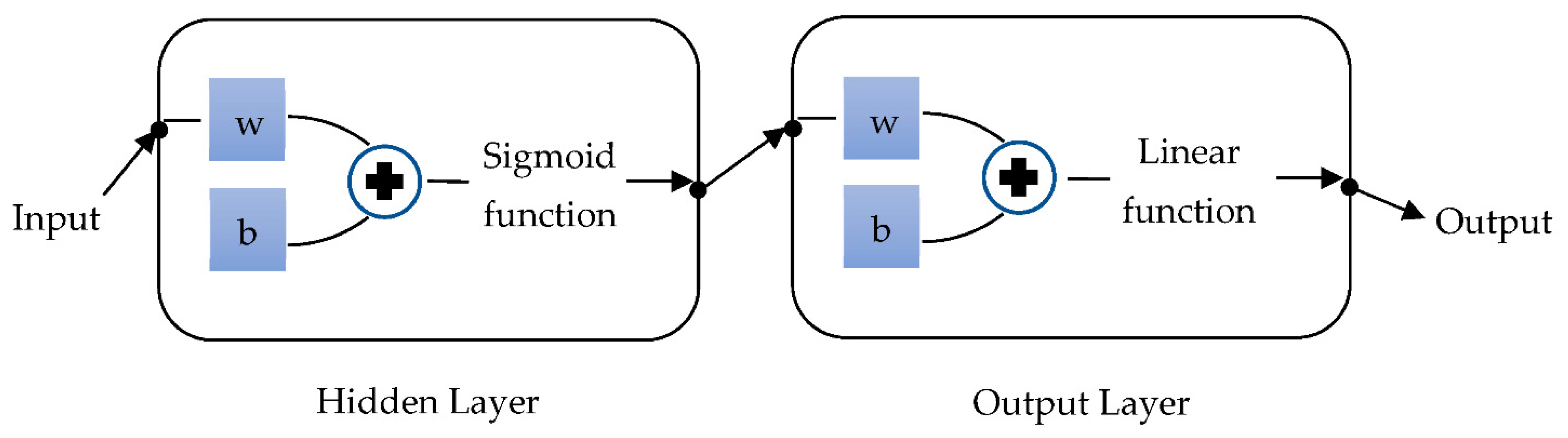
2.2. Methodology
3. Results and Discussion
4. Conclusions
Supplementary Materials
Author Contributions
Funding
Institutional Review Board Statement
Informed Consent Statement
Data Availability Statement
Conflicts of Interest
References
- Amanollahi, J.; Tzanis, C.; Abdullah, A.M.; Ramli, M.F.; Pirasteh, S. Development of the models to estimate particulate matter from thermal infrared band of Landsat Enhanced Thematic Mapper. Int. J. Environ. Sci. Technol. 2013, 10, 1245–1254. [Google Scholar] [CrossRef] [Green Version]
- Baklanov, A.; Molina, L.T.; Gauss, M. Megacities, air quality and climate. Atmos. Environ. 2016, 126, 235–249. [Google Scholar] [CrossRef]
- European Environment Agency. Air Quality in Europe—2013 Report: EEA Report No. 9/2013; European Union: Luxembourg, 2013. Available online: http://www.eea.europa.eu/publications/air-quality-in-europe-2013 (accessed on 11 November 2020).
- Grøntoft, T. Estimation of damage cost to building façades per kilo emission of air pollution in Norway. Atmosphere 2020, 11, 686. [Google Scholar] [CrossRef]
- de la Fuente, D.; Vega, J.M.; Viejo, F.; Díaz, I.; Morcillo, M. City scale assessment model for air pollution effects on the cultural heritage. Atmos. Environ. 2011, 45, 1242–1250. [Google Scholar] [CrossRef] [Green Version]
- Can, A.; Dekoninck, L.; Botteldooren, D. Measurement network for urban noise assessment: Comparison of mobile measurements and spatial interpolation approaches. Appl. Acoust. 2014, 83, 32–39. [Google Scholar] [CrossRef] [Green Version]
- Denby, B.; Sundvor, I.; Cassiani, M.; de Smet, P.; de Leeuw, F.; Horálek, J. Spatial Mapping of Ozone and SO2 Trends in Europe. Sci. Total Environ. 2010, 408, 4795–4806. [Google Scholar] [CrossRef] [PubMed]
- Li, J.; Heap, A.D. Spatial interpolation methods applied in the environmental sciences: A review. Environ. Model. Softw. 2014, 53, 173–189. [Google Scholar] [CrossRef]
- Liang, F.; Xiao, Q.; Wang, Y.; Lyapustin, A.; Li, G.; Gu, D.; Pan, X.; Liu, Y. MAIAC-based long-term spatiotemporal trends of PM2.5 in Beijing, China. Sci. Total Environ. 2018, 616–617, 1589–1598. [Google Scholar] [CrossRef]
- Yang, J.; Hu, M. Filling the missing data gaps of daily MODIS AOD using spatiotemporal interpolation. Sci. Total Environ. 2018, 633, 677–683. [Google Scholar] [CrossRef]
- Zhang, R.; Di, B.; Luo, Y.; Deng, X.; Grieneisen, M.L.; Wang, Z.; Yao, G.; Zhan, Y. A nonparametric approach to filling gaps in satellite-retrieved aerosol optical depth for estimating ambient PM2.5 levels. Environ. Pollut. 2018, 243, 998–1007. [Google Scholar] [CrossRef] [PubMed]
- Blanchard, C.L.; Tanenbaum, S.; Hidy, G.M. Spatial and temporal variability of air pollution in Birmingham, Alabama. Atmos. Environ. 2014, 89, 382–391. [Google Scholar] [CrossRef]
- Ma, J.; Cheng, J.C.P.; Lin, C.; Tan, Y.; Zhang, J. Improving air quality prediction accuracy at larger temporal resolutions using deep learning and transfer learning techniques. Atmos. Environ. 2019, 214, 116885. [Google Scholar] [CrossRef]
- Qi, Y.; Li, Q.; Karimian, H.; Liu, D. A hybrid model for spatiotemporal forecasting of PM 2.5 based on graph convolutional neural network and long short-term memory. Sci. Total Environ. 2019, 664, 1–10. [Google Scholar] [CrossRef] [PubMed]
- Vakili, M.; Sabbagh-Yazdi, S.R.; Khosrojerdi, S.; Kalhor, K. Evaluating the effect of particulate matter pollution on estimation of daily global solar radiation using artificial neural network modeling based on meteorological data. J. Clean. Prod. 2017, 141, 1275–1285. [Google Scholar] [CrossRef]
- Zainuddin, Z.; Pauline, O. Modified wavelet neural network in function approximation and its application in prediction of time-series pollution data. Appl. Soft Comput. J. 2011, 11, 4866–4874. [Google Scholar] [CrossRef]
- Coman, A.; Ionescu, A.; Candau, Y. Hourly ozone prediction for a 24-h horizon using neural networks. Environ. Model. Softw. 2008, 23, 1407–1421. [Google Scholar] [CrossRef]
- Chattopadhyay, S. Feed forward Artificial Neural Network model to predict the average summer-monsoon rainfall in India. Acta Geophys. 2007, 55, 369–382. [Google Scholar] [CrossRef]
- Wahid, H.; Ha, Q.P.; Duc, H.; Azzi, M. Neural network-based meta-modelling approach for estimating spatial distribution of air pollutant levels. Appl. Soft Comput. J. 2013, 13, 4087–4096. [Google Scholar] [CrossRef]
- Cheng, J.C.P.; Ma, L.J. A data-driven study of important climate factors on the achievement of LEED-EB credits. Build. Environ. 2015, 90, 232–244. [Google Scholar] [CrossRef]
- Yang, Z.; Wang, J. A new air quality monitoring and early warning system: Air quality assessment and air pollutant concentration prediction. Environ. Res. 2017, 158, 105–117. [Google Scholar] [CrossRef] [PubMed]
- Zhan, D.; Kwan, M.P.; Zhang, W.; Yu, X.; Meng, B.; Liu, Q. The driving factors of air quality index in China. J. Clean. Prod. 2018, 197, 1342–1351. [Google Scholar] [CrossRef]
- Silva, L.T.; Mendes, J.F.G. City Noise-Air: An environmental quality index for cities. Sustain. Cities Soc. 2012, 4, 1–11. [Google Scholar] [CrossRef]
- Ganguly, N.D.; Tzanis, C.G.; Philippopoulos, K.; Deligiorgi, D. Analysis of a severe air pollution episode in India during Diwali festival—A nationwide approach. Atmósfera 2019, 32, 225–236. [Google Scholar] [CrossRef] [Green Version]
- Tzanis, C.G.; Koutsogiannis, I.; Philippopoulos, K.; Deligiorgi, D. Recent climate trends over Greece. Atmos. Res. 2019, 230, 104623. [Google Scholar] [CrossRef]
- Tzanis, C.G.; Alimissis, A.; Philippopoulos, K.; Deligiorgi, D. Applying linear and nonlinear models for the estimation of particulate matter variability. Environ. Pollut. 2019, 246, 89–98. [Google Scholar] [CrossRef]
- Varotsos, C.; Christodoulakis, J.; Tzanis, C.; Cracknell, A.P. Signature of tropospheric ozone and nitrogen dioxide from space: A case study for Athens, Greece. Atmos. Environ. 2014, 89, 721–730. [Google Scholar] [CrossRef]
- Tzanis, C.; Varotsos, C.A. Tropospheric aerosol forcing of climate: A case study for the greater area of Greece. Int. J. Remote Sens. 2008, 29, 2507–2517. [Google Scholar] [CrossRef]
- Willmott, K.; Matsuura, K. Advantages of the mean absolute error (MAE) over the root mean square error (RMSE) in assessing average model performance. Clim. Res. 2005, 30, 79–82. [Google Scholar] [CrossRef]
- Alimissis, A.; Philippopoulos, K.; Tzanis, C.G.; Deligiorgi, D. Spatial estimation of urban air pollution with the use of artificial neural network models. Atmos. Environ. 2018, 191, 205–213. [Google Scholar] [CrossRef]
- Fallahi, S.; Amanollahi, J.; Tzanis, C.G.; Ramli, M.F. Estimating solar radiation using NOAA/AVHRR and ground measurement data. Atmos. Res. 2018, 199, 93–102. [Google Scholar] [CrossRef]
- Rahimpour, A.; Amanollahi, J.; Tzanis, C.G. Air quality data series estimation based on machine learning approaches for urban environments. Air Qual. Atmos. Health 2021, 14, 191–201. [Google Scholar] [CrossRef]
- Mirzaei, M.; Amanollahi, J.; Tzanis, C.G. Evaluation of linear, nonlinear, and hybrid models for predicting PM2.5 based on a GTWR model and MODIS AOD data. Air Qual. Atmos. Health 2019, 12, 1215–1224. [Google Scholar] [CrossRef]


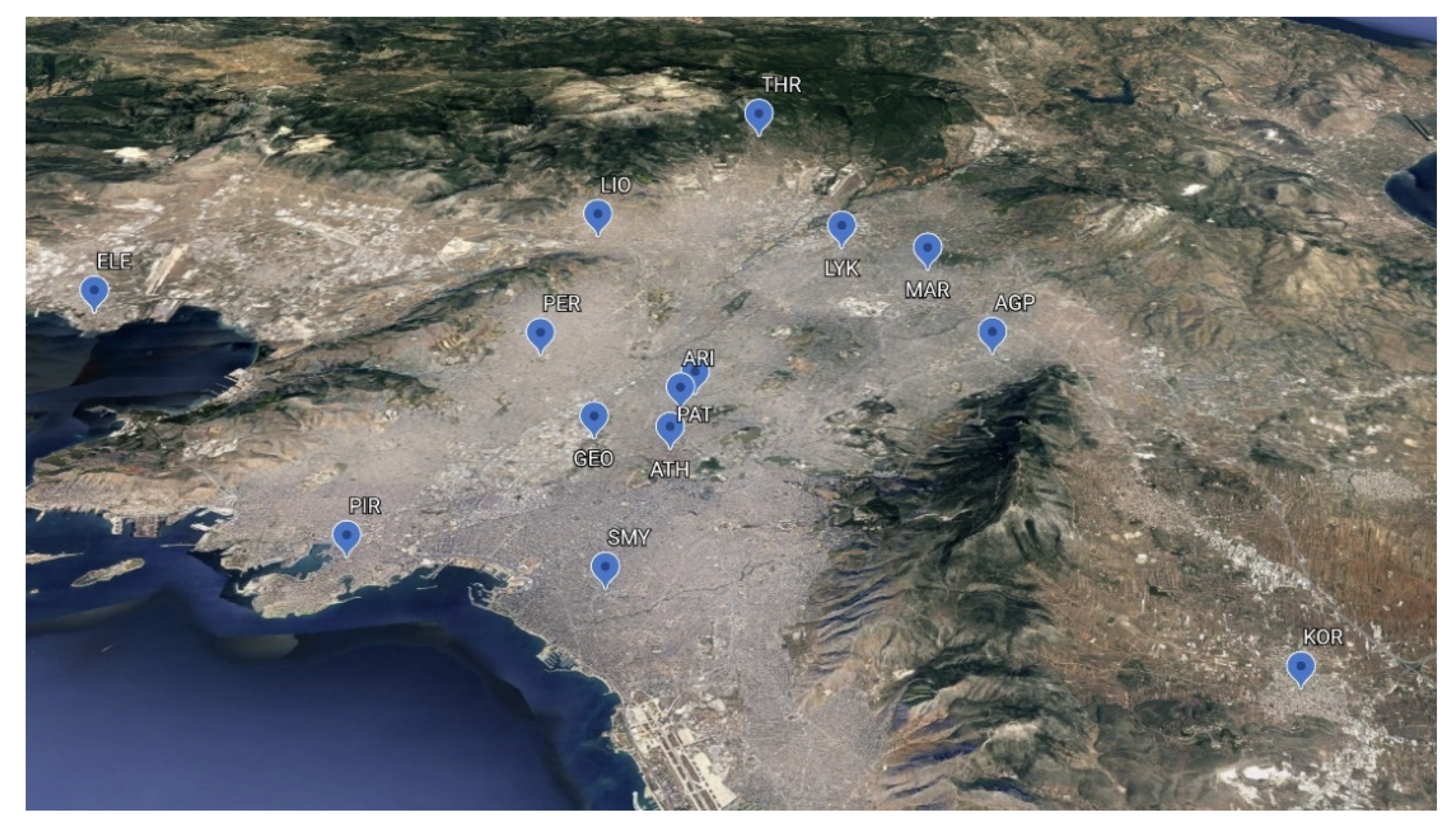
| Station | Abbreviation | Type |
|---|---|---|
| Ag. Paraskevi | AGP | Suburban/Background |
| Athinas | ATH | Urban/Traffic |
| Aristotelous | ARI | Urban/Traffic |
| Geoponiki | GEO | Suburban/Industrial |
| Elefsina | ELE | Suburban/Industrial |
| Thrakomakedones | THR | Suburban/Background |
| Koropi | KOR | Suburban/Background |
| Liosia | LIO | Suburban/Background |
| Lykovrisi | LYK | Suburban/Background |
| Marousi | MAR | Urban/Background |
| N. Smyrni | SMY | Urban/Background |
| Patission | PAT | Urban/Traffic |
| Piraeus | PIR | Urban/Traffic |
| Peristeri | PER | Urban/Background |
| Original Gaps | Gaps after Interpolation | Difference | Estimated Percentage (%) | |
|---|---|---|---|---|
| NO2 | 13,253 | 11,145 | 2108 | 15.91 |
| O3 | 10,814 | 7961 | 2853 | 26.38 |
| PM10 | 7182 | 3948 | 3234 | 45.03 |
| PM2.5 | 4558 | 2524 | 2034 | 44.62 |
| SO2 | 7043 | 4746 | 2297 | 32.61 |
| Training | Validation | Testing | Total | |
|---|---|---|---|---|
| NO2 | 47,151 | 10,101 | 10,101 | 67,353 |
| O3 | 25,272 | 5412 | 5412 | 36,096 |
| PM10 | 13,410 | 2880 | 2880 | 19,170 |
| PM2.5 | 37,785 | 8100 | 8100 | 53,985 |
| SO2 | 13,925 | 3080 | 3080 | 20,085 |
| Number of Neurons | MAE | RMSE | R2 | ||||||||
|---|---|---|---|---|---|---|---|---|---|---|---|
| Input | Hidden | Output | Mean | ANNs | Error (%) | MLR | ANNs | MLR | ANNs | MLR | |
| NO2 | 13 | 21.7 | 1 | 32.70 | 5.80 | 17.74 | 7.23 | 8.31 | 9.87 | 0.76 | 0.67 |
| O3 | 12 | 22.3 | 1 | 58.86 | 6.86 | 11.65 | 9.32 | 9.78 | 12.49 | 0.87 | 0.77 |
| PM10 | 10 | 23.6 | 1 | 29.53 | 5.71 | 19.34 | 7.17 | 11.55 | 11.65 | 0.88 | 0.87 |
| PM2.5 | 5 | 25.2 | 1 | 23.81 | 5.17 | 21.71 | 5.68 | 8.47 | 8.97 | 0.69 | 0.65 |
| SO2 | 5 | 22.5 | 1 | 6.06 | 1.89 | 31.19 | 2.39 | 3.29 | 3.74 | 0.55 | 0.39 |
| Mean | Mean Error | Variance | Variance Error | |||
|---|---|---|---|---|---|---|
| O | I | O | I | |||
| AGP | 14.06 | 14.06 | −1.83 × 10⁻⁶ | 147.91 | 147.86 | −3.53 × 10⁻⁴ |
| ATH | 44.24 | 42.90 | −0.03 | 377.36 | 387.47 | 0.03 |
| ARI | 47.95 | 47.95 | −5.35 × 10⁻⁵ | 405.37 | 405.23 | −3.45 × 10⁻⁴ |
| GEO | 28.01 | 27.99 | −7.81 × 10⁻⁴ | 326.76 | 311.44 | −0.05 |
| ELE | 24.41 | 24.42 | 2.99 × 10⁻⁴ | 204.55 | 204.82 | 13 × 10−4 |
| THR | 7.96 | 7.68 | −0.04 | 94.85 | 87.34 | −0.08 |
| KOR | 8.26 | 8.35 | 0.01 | 183.60 | 184.53 | 0.01 |
| LIO | 16.68 | 16.69 | 7.88 × 10⁻⁴ | 187.13 | 187.86 | 39 × 10−4 |
| LYK | 19.98 | 20.01 | 11 × 10−4 | 286.24 | 284.08 | −0.01 |
| MAR | 26.40 | 26.40 | −8.63 × 10⁻⁶ | 466.69 | 466.59 | −2.17 × 10⁻⁴ |
| SMY | 29.16 | 29.23 | 25 × 10−4 | 480.56 | 483.84 | 0.01 |
| PAT | 70.95 | 70.94 | −1.59 × 10⁻⁴ | 750.28 | 750.33 | 6.07 × 10⁻⁵ |
| PIR | 62.53 | 62.53 | −4.43 × 10⁻⁵ | 602.95 | 603.12 | 2.82 × 10⁻⁴ |
| PER | 27.69 | 27.69 | −7.61 × 10⁻⁵ | 462.81 | 462.49 | −6.80 × 10⁻⁴ |
| Mean | Mean Error | Variance | Variance Error | |||
|---|---|---|---|---|---|---|
| O | I | O | I | |||
| AGP | 82.61 | 82.66 | 5.05 × 10⁻⁴ | 804.22 | 809.52 | 0.01 |
| ATH | 40.50 | 40.50 | 1.28 × 10⁻⁵ | 882.74 | 882.54 | −2.26 × 10⁻⁴ |
| GEO | 56.27 | 59.01 | 0.05 | 1329.6 | 1334.4 | 36 × 10−4 |
| ELE | 63.78 | 63.60 | −29 × 10−4 | 1226 | 1226 | −6.03 × 10⁻⁵ |
| THR | 96.50 | 96.51 | 1.24 × 10⁻⁴ | 677.91 | 678.06 | 2.10 × 10⁻⁴ |
| KOR | 65.77 | 65.77 | −2.58 × 10⁻⁵ | 607.77 | 608.73 | 16 × 10−4 |
| LIO | 64.71 | 65.33 | 0.01 | 1199.8 | 1193.3 | −0.01 |
| LYK | 64.42 | 64.07 | −0.01 | 1352.1 | 1344.6 | −0.01 |
| MAR | 65.81 | 65.88 | 11 × 10−4 | 1387.2 | 1348.5 | −0.03 |
| SMY | 73.65 | 73.87 | 30 × 10−4 | 1314.2 | 1318.6 | 33 × 10−4 |
| PAT | 16.52 | 16.83 | 0.02 | 278.29 | 296.92 | 0.07 |
| PIR | 40.45 | 40.43 | −3.74 × 10⁻⁴ | 944.15 | 943.88 | −2.90 × 10⁻⁴ |
| PER | 66.04 | 66.43 | 0.01 | 1385.3 | 1388.4 | 23 × 10−4 |
| Mean | Mean Error | Variance | Variance Error | |||
|---|---|---|---|---|---|---|
| O | I | O | I | |||
| AGP | 19.85 | 19.83 | −7.09 × 10⁻⁴ | 432.11 | 429.55 | −0.01 |
| ARI | 36.38 | 36.37 | −3.18 × 10⁻⁴ | 630.70 | 628.58 | −33 × 10−4 |
| ELE | 29.27 | 29.06 | −0.01 | 488.50 | 479.02 | −0.02 |
| THR | 20.40 | 20.44 | 18 × 10−4 | 414.02 | 401.35 | −0.03 |
| KOR | 30.72 | 30.67 | −16 × 10−4 | 601.64 | 597.62 | −0.01 |
| LIO | 33.74 | 32.93 | −0.02 | 806.56 | 704.83 | −0.13 |
| LYK | 27.03 | 27.63 | 0.02 | 378.55 | 657.21 | −0.74 |
| MAR | 29.48 | 29.48 | 7.46 × 10⁻⁵ | 685.14 | 680.14 | −0.01 |
| SMY | 31.03 | 30.79 | −0.01 | 666.01 | 644.88 | −0.03 |
| PIR | 39.34 | 39.49 | 37 × 10−4 | 695.72 | 697.59 | 27 × 10−4 |
| PER | 30.31 | 30.32 | 2.16 × 10⁻⁴ | 713.39 | 707.80 | −0.01 |
| Mean | Mean Error | Variance | Variance Error | |||
|---|---|---|---|---|---|---|
| O | I | O | I | |||
| AGP | 11.60 | 11.60 | −4.47 × 10⁻⁴ | 42.35 | 42.17 | −42 × 10−4 |
| ARI | 19.11 | 18.92 | −0.01 | 213.67 | 204.40 | −43 × 10−4 |
| ELE | 17.81 | 17.83 | 9.18 × 10⁻⁴ | 100.90 | 99.98 | −92 × 10−4 |
| THR | 13.44 | 13.43 | −10 × 10−4 | 45.47 | 44.63 | −186 × 10−4 |
| LYK | 15.28 | 15.47 | 0.01 | 133.63 | 133.81 | 14 × 10−4 |
| PIR | 18.00 | 18.24 | 0.01 | 178.46 | 183.70 | 29 × 10−4 |
| Mean | Mean Error | Variance | Variance Error | |||
|---|---|---|---|---|---|---|
| O | I | O | I | |||
| ATH | 4.21 | 4.21 | 15 × 10−4 | 12.22 | 12.29 | 53 × 10−4 |
| ARI | 4.46 | 4.58 | 265 × 10−4 | 11.57 | 11.70 | 109 × 10−4 |
| ELE | 10.73 | 10.57 | −150 × 10−4 | 45.35 | 47.76 | 529 × 10−4 |
| KOR | 4.92 | 4.91 | −25 × 10−4 | 7.49 | 7.45 | −51 × 10−4 |
| PAT | 8.87 | 8.85 | −28 × 10−4 | 20.17 | 20.20 | 14 × 10−4 |
| PIR | 9.93 | 9.92 | −13 × 10−4 | 66.21 | 65.52 | −105 × 10−4 |
Publisher’s Note: MDPI stays neutral with regard to jurisdictional claims in published maps and institutional affiliations. |
© 2021 by the authors. Licensee MDPI, Basel, Switzerland. This article is an open access article distributed under the terms and conditions of the Creative Commons Attribution (CC BY) license (https://creativecommons.org/licenses/by/4.0/).
Share and Cite
Tzanis, C.G.; Alimissis, A.; Koutsogiannis, I. Addressing Missing Environmental Data via a Machine Learning Scheme. Atmosphere 2021, 12, 499. https://doi.org/10.3390/atmos12040499
Tzanis CG, Alimissis A, Koutsogiannis I. Addressing Missing Environmental Data via a Machine Learning Scheme. Atmosphere. 2021; 12(4):499. https://doi.org/10.3390/atmos12040499
Chicago/Turabian StyleTzanis, Chris G., Anastasios Alimissis, and Ioannis Koutsogiannis. 2021. "Addressing Missing Environmental Data via a Machine Learning Scheme" Atmosphere 12, no. 4: 499. https://doi.org/10.3390/atmos12040499