Article

Relationship between Changes over Time in Factors, Including the Impact of Meteorology on Photochemical Oxidant Concentration and Causative Atmospheric Pollutants in Kawasaki

1
Kawasaki Environment Research Institute (KERI), Kanagawa, Kawasaki 210-0821, Japan
2
Kawasaki City Environment Bureau, Kanagawa, Kawasaki 210-8577, Japan
3
Institute of Integrated Atmospheric Environment (IIAE), Ehime University, Ehime, Matsuyama 790-8566, Japan
*
Author to whom correspondence should be addressed.
Atmosphere 2021, 12(4), 446; https://doi.org/10.3390/atmos12040446
Submission received: 12 February 2021 / Revised: 15 March 2021 / Accepted: 28 March 2021 / Published: 31 March 2021
(This article belongs to the Special Issue Air Pollution in Japan)

Abstract

:
To clarify the relationship between changes in photochemical oxidants’ (Ox) concentrations and their precursors in Kawasaki, a series of analyses were conducted using data on Ox, their precursors, nitrogen oxides (NOx) and volatile organic compounds (VOCs), and meteorology that had been monitored throughout the city of Kawasaki for 30 years from 1990 to 2019. The trend in air temperature was upward, wind speed was downward, and solar radiation was upward, indicating an increasing trend in meteorological factors in which Ox concentrations tend to be higher. Between 1990 and 2013, the annual average Ox increased throughout Kawasaki and remained flat after that. The three-year moving average of the daily peak increased until 2015, and after that, it exhibited a slight decline. The amount of generated Ox is another important indicator. To evaluate this, a new indicator, the daytime production of photochemical oxidant (DPOx), was proposed. DPOx is defined by daytime averaged Ox concentrations less the previous day’s nighttime averaged Ox concentrations. The trend in DPOx from April to October has been decreasing since around 2006, and it was found that this indicator reflects the impact of reducing emissions of NOx and VOCs in Kawasaki.

1. Introduction

Kawasaki is part of the Keihin (Tokyo–Yokohama, Japan) industrial area, and therefore industries such as steel, chemical, and petrochemical are concentrated in the city. At one time, the city experienced serious pollution problems, such as atmospheric pollution and water contamination, but in 1972, the Kawasaki city government implemented local regulations for total pollution loads (Appendix A) first in Japan, and in 1974, the Environment Agency, government of Japan (later Ministry of the Environment, Tokyo, Japan), implemented similar regulations. As such, it is a city that has been a pioneer in Japan of advanced measures to control air pollution. As a result, in fiscal year (FY)2019, the average concentration of SO2 had dropped by 99% from its peak in FY1965, while the average concentration of CO had fallen by 92% compared with its FY1972 peak. Data like these illustrate that there has been a huge improvement in the concentrations of primary pollutants.
In contrast, in Japan, the environmental quality standard (EQS) for photochemical oxidants (Ox) (shown in Table 1) was established in 1973, and Ox exceed the EQS nationwide, including in Kawasaki.
Ox are defined as oxidizing substances in the atmosphere, excluding NOx. However, ozone (O3) is the major component of Ox, so the Ministry of the Environment (MOE), government of Japan, decided to equate O3 concentrations with Ox concentrations in 1996 [1]. In this paper, O3 is used interchangeably Ox.
The dynamics of Ox in urban and surrounding areas are closely related to meteorological parameters such as the intensity of ultraviolet (UV) radiation, air temperature, wind speed, and wind direction. High concentrations of Ox in summer result in the frequent occurrence of photochemical smog [2], where the air turns white and hazy. This can have an adverse impact on human respiratory organs and on plant life [3,4]. Atmospheric pollutants, including Ox, are accelerating factors in the material deterioration of buildings and other structures as well as objects of cultural heritage. Relationships between air pollution and material deterioration were investigated [5]. Observations of O3 had already been conducted in the first half of the 20th century, and the measurements were re-evaluated using the original conversion method [6]. The observed O3, NO, NO2, and NOx were statistically analyzed, and original numerical relations were devised using the data [7,8]. In urban areas around Kawasaki, trend analyses of precursors of O3 [9], analyses on the impact of the previous day’s precursors with three-dimensional simulation models [10], and analyses of the relationship between precursor emissions and O3 concentrations [11] were conducted. Nationwide, a comparison of results calculated with four gas-phase chemical mechanisms involved in ozone formation [12], evaluation of model performance on ozone concentrations over urban areas in model inter-comparisons [13], and comprehensive analyses of source sensitivities and apportionments of ozone via multiple numerical techniques [14] were conducted. In other countries, analyses of the relationship between O3 concentrations and trends in precursors of O3 have been conducted [15,16].
In addition to the EQS, the MOE proposed a new indicator, the three-year moving average of the annual 99th percentile of the daily maximum for the eight-hour value of Ox (Appendix B). However, this indicator is often strongly influenced by transboundary pollutants because of meteorological conditions. So, a new indicator independent of meteorological conditions is essential to assess the amount of Ox formation in a local area. In this article, trend analyses of 30 years of observed data on Ox, NOx, non-methane hydrocarbons (NMHC) (an indicator of volatile organic compounds (VOCs)), and meteorology in Kawasaki are conducted. Furthermore, an original indicator representing the amount of Ox formation in Kawasaki is proposed. This indicator represents the amount of Ox formation independent of meteorological condition changes by year and can be using to assess the effectiveness of strategies for reducing ozone precursor emissions.

2. Monitoring of Atmospheric Pollution and the Trend in Ox Concentrations

2.1. Monitoring of Atmospheric Pollution

In this article, we will refer to the region that contains the city of Tokyo and the prefectures of Kanagawa, Chiba, and Saitama, which is shown in Figure 1, as the Tokyo Metropolitan Area (TMA). Kawasaki is a city located in the northern part of Kanagawa, which itself is situated in the southwestern part of the TMA. The city covers an area of 144 km2 and borders the southern part of Tokyo at the north. The southeast of the city faces Tokyo Bay (Honshu, Japan), and the coastal area is part of the Keihin industrial area, which is one of Japan’s foremost industrial zones.
Geographically, ground elevation increases gradually as one moves inland from the coastal area, and land reaches its highest point above sea level, 140 m, approximately 27 km from the sea. The city is also an important transport hub connecting the huge city of Tokyo, Japan’s capital, with Kanagawa Prefecture, making it a highly convenient location. This has attracted numerous residents, and the population currently stands at over 1.5 million, making the city Japan’s sixth largest in terms of population.
In this environment, air quality is well maintained, and with the aim of protecting the health of residents, atmospheric pollution is monitored continuously in Kawasaki.
Figure 2 shows the air monitoring system in operation in Kawasaki. For this paper, we employed constant-observation data from all 18 stations that were used, as of October 2020, to take measurements in Kawasaki. These comprise nine general stations (General sta., explained in the description of administrative criteria) and nine roadside stations (Roadside sta., explained in the description of administrative criteria).
The period of analysis was 30 years from FY1990 to FY2019, and the variables surveyed were Ox, NOx (total of NO and NO2), NMHC, and climate (air temperature, solar radiation, and wind speed). In this paper, fiscal year (FY) denotes a period from April of a year until March of the following year, while year denotes a period from January to December.
Ox is monitored at all 9 General sta.; NOx, which is the total of NO2 and NO, is monitored at all 18 General sta. and Roadway sta.; NMHC are monitored at 7 General sta., excluding Miyamae and Asao; air temperature and wind speed are monitored at all 9 General sta.; and solar radiation is monitored at just 2 stations, Tajima and Saiwai.
Even as part of the TMA, Kawasaki covers only a limited area and is regarded as a single, self-contained area, so we based our analysis not on the measurements from each station but on the average values from all the stations.

2.2. Trend in Ox Concentrations

2.2.1. Annual Average

Figure 3 shows the trend in the annual average Ox calculated as the average of hourly values for all nine general air monitoring/measurement stations installed in Kawasaki. The three lines (All the time, Daytime, and Night) refer, respectively, to the 24 h average, the average for 6 a.m.–8 p.m., and the average for 12 a.m.–5 a.m. and 9 p.m.–12 a.m.
The three annual averages generally all exhibited an upward trend from FY1990, and the tendency for daytime Ox concentrations to increase was similar to that seen with the nationwide average [17]. The averages also remained flat from around FY2013 onward.
The trend over time in the monthly average Ox for each month was investigated to obtain a detailed breakdown of the annual average, and the results are shown in Figure 4. It became clear that Ox concentrations in spring, which is in April and May, are higher than those in other seasons and these concentrations have markedly increased over the years. Transboundary transport from the continent is likely to be the reason for the high Ox concentrations seen in April and May [18,19].
To quantitatively grasp the rise in Ox over the years, the year-on-year rate of increase in the monthly average Ox for each decade is shown in Figure 5. In the 1990s, there was an upward trend in all months except July. In the 2000s, January and December exhibited a slight downward trend, but the trend was upward for the other months and during the period from April to October, during which photochemical smog warnings (PSW) are issued, the upward trend was comparatively higher in May and September. In the 2010s, the trend was upward for all months with the exception of July.

2.2.2. The Number of Days on Which Photochemical Smog Warnings Issued

In Japan, if the hourly value of Ox is 0.12 ppm or higher and the meteorological condition average of this situation is expected to continue, the prefectural governor issues, pursuant to the Air Pollution Control Act, photochemical smog warnings (PSW) to raise awareness among citizens and urge factories to take steps such as reducing their fuel usage (Appendix C). In the TMA, PSW are issued every year, mainly during summer, and smog has become a serious issue relating to the air environment [20].
As an indicator of high Ox concentrations, the trend over time in the number of days on which PSW were issued in Kawasaki is shown in Figure 6. Regarding the number of days on which PSW were issued, in the 1990s, the number did not exceed 10 days in any fiscal year, so the number was comparatively small. In the 2000s, however, the number of PSW topped 10 in FY2001, FY2004, FY2006, and FY2007, with the peak being in FY2007, when the number of such days was 13. In the 2010s, the number of PSW surpassed 10 only in FY2013, so a decline was seen relative to the 2000s. Over the entire 30-year period, the level of fiscal-year-to-fiscal-year variation in the number of PSW was large.
As an indicator of high Ox concentrations throughout the year, the annual averages of daytime daily maximums are shown in Figure 7. Because the daily maximum is prone to influence by meteorological conditions, it is shown as a three-year moving average. Although an upward trend was seen until around FY2015, it has remained flat in recent years.

2.2.3. A New Indicator from the MOE

In 2016, the MOE presented the three-year moving average of the annual 99th percentile of the daily maximum for the eight-hour value as an indicator for properly assessing the effectiveness of Ox-related environmental improvements (Appendix B). The 99th percentile of the daily maximum for the eight-hour value involves calculating the maximum from among the eight-hour moving averages on a single day. A year’s worth of these maximum values is arranged, and the 99% counting from the lowest day is the 99th percentile of the daily maximum for the eight-hour value. It is suitable for determining the situation in a high-concentration zone. This value has been on a downward trend since around FY2008 in the TMA, Nagoya area, Osaka/Kyoto area, and Kyushu area [21]. Figure 8 shows the application of this indicator to the average from all nine General sta. that perform measurements in Kawasaki. Peaks were also seen in Kawasaki around FY2008; after that, there is variation over time, depending on the fiscal year and the value is flat. FY2013 was an unusual fiscal year, as during summer, high pressure over the Pacific was combined with high pressure over Tibet, and these high-pressure systems covered the whole of Japan. As a result, air temperatures were high, solar radiation was high, and wind speed was slow [22]. In FY2017–FY2019, meanwhile, we believe that the new indicator increased due to the impact of the nationwide transboundary pollution that occurred in May 2019 [23].

3. Meteorological Conditions

Because Ox is a secondary pollutant generated by ultraviolet (UV) radiation, the development of high concentrations is closely related to meteorological factors such as air temperature, wind speed, and solar radiation [2]. Because of this, long-term trends in factors such as air temperature, wind speed, and solar radiation in Kawasaki were analyzed over 30 years from 1990 to 2019.

3.1. Air Temperature
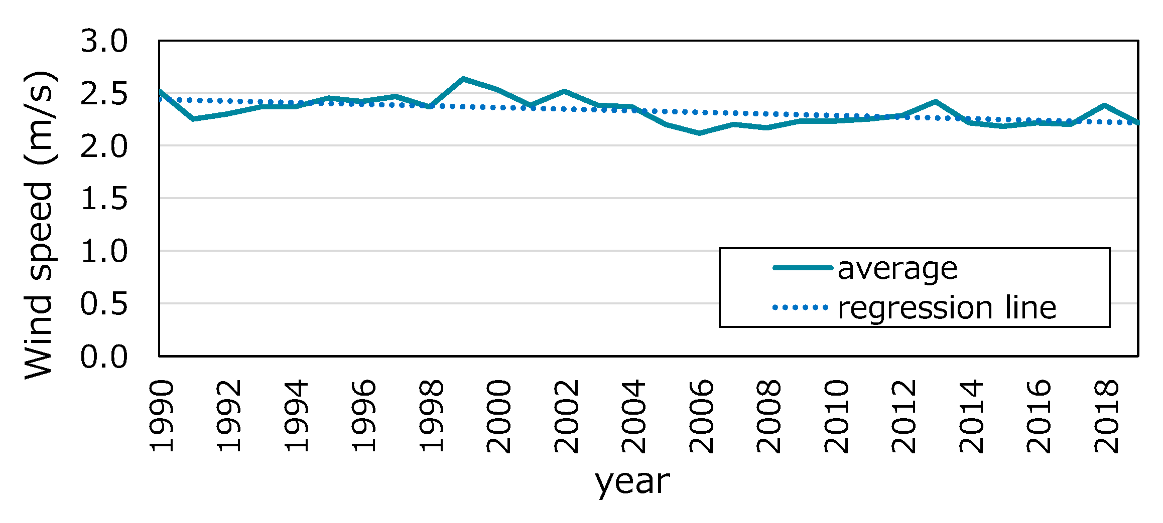
The trends in the annual averages of the daily maximum temperature, daily average temperature, and daily minimum temperature are shown in Figure 9. All of them exhibit a rising trend, and the rate of increase in the minimum temperature is the greatest (0.00338 °C/year), which is followed by the rate of increase in the average temperature (0.0274 °C/year) and the rate of increase in the maximum temperature (0.0234 °C/year), as seen from the slopes of the regression lines.
The rate of increase over time in the monthly average temperature is shown in Figure 10. The daily minimum temperature and the daily average temperature trend upward for all months, and the daily maximum temperature exhibits a rising trend in every month except February, November, and December. The rates of increase from March to October are greater than those for January, February, November, and December, which indicates that winters are shorter and summers are longer. From April to October, the period during which PSW are issued, the rising trend is particularly marked.

3.2. Wind Speed

The trend in the annual average wind speed is shown in Figure 11. Wind speed data of six stations continuously operated were used for analyzing. Although there was year-to-year variation between 1990 and 2019, a gradual declining trend was observed.
The rate of increase over time in the monthly average wind speed for each month is shown in Figure 12. A declining trend is seen in every month. During the period April–October, when PSW are issued, the downward trend is greater than the annual average in May, June, August, and September and smaller than the annual average in July.

3.3. Solar Radiation

The trends in the annual averages of solar radiation compared with those of air temperature are shown in Figure 13. Solar radiation exhibited a rising trend between 1990 and 2019, and it could be said that there has been an increase in the tendency of photochemical reactions to occur. Trends of an increase/decrease in solar radiation and air temperature approximately matched.
The rate of increase in solar radiation for each month is shown in Figure 14. An increasing trend is observed in all the months, with a particularly large rate of increase in March and May. During April–October, when PSW are issued, the rate of increase is the highest in May, followed by April.
As shown above, having analyzed the air temperature, solar radiation, and wind speed in Kawasaki between 1990 and 2019, because air temperature and solar radiation exhibited an upward trend and wind speed exhibited a downward trend, it can be said that for each of the parameters air temperature, solar radiation, and wind speed, during the period from April to October, when PSW are issued, from these meteorological points of view, the Ox formation potential has been increasing.

4. Precursors

4.1. NOx

4.1.1. Emissions of NOx

Nitrogen oxides from anthropogenic sources are mainly generated through the combustion of fossil fuels and are mainly emitted by stationary sources such as factories and workplaces and mobile sources such as motor vehicles.
The trend over time in the emissions of NOx from factories and workplaces (which contain facilities that emit soot and smoke (boilers, etc.) defined by the Air Pollution Control Act) in Kawasaki is shown in Figure 15. For the volume of NOx emissions from facilities that emit soot and smoke, aggregated results of reported emissions from stationary sources in Kawasaki were used. The volume of NOx emitted from factories and workplaces in FY2018 declined by 33% compared with that in FY1990. Furthermore, in FY2000, the Kawasaki city government established its own comprehensive total emissions control scheme (Appendix D). Full implementation of the scheme was achieved in FY2005, and reductions in NOx emission have increased substantially.
The trend over time in the emissions of NOx from motor vehicles driven in Kawasaki is shown in Figure 16. The value of the emissions of NOx was produced from the estimates reported by the Kawasaki city government, though it only covers fiscal years for which data on traffic density could be obtained. The emissions of NOx from motor vehicles remained steady from FY1993 to FY1997 but began to decline in FY1997. The emissions in FY2015 dropped by 27% compared with those in FY1997. In Japan, vehicle-specific regulations that apply at the time of new-vehicle registrations and vehicle-type regulations that apply at the time of vehicle inspections are being tightened in phases. In the TMA, regulations concerning the use of diesel vehicles were introduced in FY2003. As a result of these regulations (Appendix E), progress has been made in reducing NOx emissions.

4.1.2. NOx Concentrations

The trends in the annual averages of NOx, NO, and NO2 are shown in Figure 17. NOx was measured at nine General sta. and nine Roadside sta. The annual averages of all three pollutants have been decreasing, and the decline at Roadside sta. from the 2000s is especially striking.
The trends in the annual averages of NO2/NOx are shown in Figure 18. Although the ratio of NO to NO2 immediately after the release of NOx from combustion sources is around 9:1 [24,25], in flue gas treatment devices as well as in the atmosphere, NO is oxidized to NO2, increasing NO2 as a proportion of NOx. As a result, NO2 as a proportion of NOx tends to be higher at General sta. than at Roadside sta. In addition, the annual averages of NO2/NOx have been on an upward trend since the year 2000.
Because NO2 is an important precursor to O3, it is extremely significant to know the ratio of NO and NO2 in NOx from the source. Because the oxidation of NO to NO2 in the atmosphere occurs by ozone or RO2 radicals, we analyzed changes over time at night (from 8 p.m. until 5 a.m.) during the cold season (from October to March), when O3 or RO2 radicals reduce. The results of this analysis are shown in Figure 19.
To investigate the trend in NOx emissions from motor vehicles in Kawasaki, the average of NOx, NO2, and NO at Roadside sta. less that at General sta. at night during the cold season is shown in Figure 20. Although NOx values stayed fairly level until FY2000, they decreased sharply after that.
To estimate the trend in NO2/NOx in NOx emitted from motor vehicles, changes over time in the average for Roadside sta. less that for General sta. at night during the cold season in Kawasaki are shown in Figure 21.
NOx emissions from motor vehicles shown in Figure 17 declined from FY1997. However, NO2/NOx emissions increased significantly from FY2005. Therefore, it seems that as NOx emissions from motor vehicles fell, NO2 as a proportion of NOx rose substantially.
Until about FY2005, NO2/NOx emissions were around 0.1, but after that, they increased to 0.3 or thereabouts, and the fact that this was identified for the first time is significant. Until now, 0.1 has generally been used as an input ratio value for NO2 as a proportion of NOx in NO emissions from motor vehicles with the atmospheric chemical transport model (CTM), but this finding shows that it needs to be altered to approximately 0.3.

4.2. NMHC

4.2.1. Emissions of NMHC

Non-methane hydrocarbons (NMHC) have been monitored as an indicator of VOCs. Estimates of emissions of VOCs from stationary sources have been published by the MOE for each prefecture since FY2000. Here, stationary sources refer to more than just factories. For example, they also include paint during construction work and vapor when filling a motor vehicle at a gas station. Trends in VOC emissions from stationary sources in Kanagawa Prefecture are shown in Figure 22. The emissions dropped sharply between FY2000 and FY2010, with the reduction in FY2010 standing at approximately 43% compared with FY2000 levels. The downward trend slowed after FY2010, yet the reduction in FY2018 compared with FY2010 was approximately 20%.
As a countermeasure to VOCs, in FY2006, the Air Pollution Control Act was amended to include new legal regulations for stationary sources that emit VOCs in large quantities. Voluntary steps to curb emissions are also being taken by business operators. This curtailment of VOC emissions through a combination of legal regulations and voluntary initiatives is referred to as the best-mix approach. The regulations for controlling VOC emissions were the first regulations to incorporate the idea of a best mix of legal regulations and voluntary cuts by businesses. For that reason, in FY2006, the Air Pollution Control Act was amended to include new legal regulations for stationary sources that emit VOCs in large quantities (Appendix F).
At the same time, a numerical target of reducing emissions by 30% by FY2010 compared with FY2000 was also set. In addition, the Kawasaki city government is working with adjacent cities in the TMA to raise awareness about reducing VOCs. These initiatives are likely contributing to the reduction in emissions.

4.2.2. NMHC Concentrations

The trend in the annual average NMHC is shown in Figure 23. NMHC are measured at seven General sta., namely Daishi, Tajima, Kawasaki, Saiwai, Nakahara, Takatsu, and Tama. With regard to NMHC, in 1976, the Environment Agency established guidelines concerning atmospheric hydrocarbon concentrations as a means of controlling the generation of Ox. Specifically, the guidelines stated that “the three-hour average of NMHC between 6 a.m. and 9 a.m. corresponding to a daily maximum hourly concentration of photochemical oxidants of 0.06 ppm should be in the range of 0.20 ppmC to 0.31 ppmC.” Therefore, the trend in the annual average of NMHC concentration was estimated using the 3 h average between 6 a.m. and 9 a.m., with that of the 24 h average as a reference. Both show a downward trend, and the figures are almost the same. Over the 30 years that are the focus of this article, the chemical component ratios in VOCs and NMHC were considerably changed. This change possibly affected the reactivity of VOCs.
It is important to consider the possibility of the effect of a change in the chemical component ratio. However, so far, the monitoring data on the chemical species are insufficient in Kawasaki.

4.3. Relationship between Ox, NOx, and NMHC

The trend in the annual averages of NMHC/NOx (ppmC/ppm) between 6 a.m. and 9 a.m. is shown in Figure 24. NMHC/NOx decreased from FY1990 to FY2004 but from FY2005 exhibited an increasing trend. The increase in NMHC/NOx from FY2005 is attributed more to the ratio of decreasing NOx than that of NMHC from FY2005.
The relationship between Ox on the one hand and NOx and NMHCs on the other from 1990 to 2019 is shown in Figure 25. In terms of decade units, both NMHC concentration and NOx concentration have been declining. On the other hand, Ox concentration has been gently rising.

5. Changes over Time in Meteorological Conditions Apt to Lead to High Concentrations

It is thought that the amount and rate of Ox production are determined by the intensity of sources of NOx and VOCs and the proportion of the two. It is conceivable that daily maximum Ox concentrations are determined by the amount of NOx emissions while the rate of Ox production is determined by the amount of VOC emissions. However, even under the same conditions of sources of NOx and VOCs, a variation in meteorological conditions such as air temperature, solar radiation, and wind speed leads to differences in temporal changes and in the geographical distribution of Ox concentrations [26,27,28,29]. Therefore, when assessing the impact of measures on sources, it is necessary to exclude variable factors due to meteorological conditions. Only the first half may be quoted. The second half is still being confirmed.
As already stated, even though both NOx concentrations and NMHC concentrations, which are causes of Ox, are declining, no downward trend in Ox concentrations is seen. However, the relationship between Ox and its precursors may not be accurately assessed under different meteorological conditions because of variations in meteorological parameters year to year, as described in Section 3.3. Consequently, the relationship between Ox and its precursors was analyzed to eliminate meteorological bias by using data of days selected by certain meteorological conditions.

5.1. Method of Selection of Meteorological Conditions Apt to Lead to High Ox Concentrations

We selected certain meteorological conditions that are likely to result in high concentrations of Ox. These meteorological conditions, air temperature, wind speed, and solar radiation, are presented in Table 2. Pattern A meets only (1); pattern B meets (1) and (2); and pattern C meets all of (1), (2), and (3).
The trend over time in the number of days matching each pattern and the trend over time in the daily maximum Ox are shown in Figure 26. As for the number of days, B had fewer days than A, but B and C were the same mostly. Below, days corresponding to pattern C will be referred to as extracted days.
The three-year average of the daily maximum Ox peaked in FY2007, after which it began to decline. From FY2012, however, it turned upward once again, before dipping again in FY2015 and remaining steady thereafter. The number of extracted days has been on an upward trend, and from FY2010, the number of extracted days consecutively topped 30 days. However, no correlation was observed between the number of extracted days and the single-year daily maximum Ox.

5.2. Relationship between Ox, NOx, and NMHC on Extracted Days

On extracted days, the relationship between Ox, NOx, and NMHC is shown in Figure 27. In terms of decade units, both NMHC and NOx declined. However, no correlation was observed between Ox, NOx, and NMHCs.
A relationship diagram of NMHC and NOx all year (Figure 25) and on extracted days (Figure 27) between FY1990 and FY2019 is also shown in Figure 28. Extracted days, upon which meteorological conditions are likely to lead to high concentrations of Ox, tend to exhibit high NMHC concentrations and low NOx concentrations compared with the all-year figures. The NMHC concentration is susceptible to the influence of stationary sources; increases in air temperature raise the volatilization of VOCs, and the concentration elevates when dispersion is suppressed due to the emergence of inversion layers or low wind speed. NMHC concentrations on extracted days, which are limited to days on which the air temperature is high and wind speed is low, tend to be higher than is the case all year round, as the entire year includes autumn and winter, when emergences of inversion layers are a frequent occurrence. Such days can, therefore, be said to be highly susceptible to the influence of rising air temperatures. In contrast, NOx concentrations are apt to rise in autumn and winter, when inversion layers often emerge, so because extracted days are concentrated in the summer, the all-year figures, which include autumn and winter, tend to be higher. It is likely that due to these reasons, on extracted days, NMHC concentrations were higher than those for all year and NOx concentrations were lower than those for all year.
Furthermore, comparing Ox concentrations in Figure 25 and Figure 27, figures for extracted days exceeded the all-year figures in every year. This can be regarded as a manifestation of the result of extracting based on meteorological conditions that are likely to push Ox concentrations upward.

6. A New Indicator for the Impact of Countermeasures to Ox in Kawasaki

The EQS for Ox is one of the toughest standards in the world, and it is difficult to assess the impact of countermeasures simply by evaluating the EQS. Therefore, to assess the effectiveness of Ox-related environmental improvements, the MOE proposed a new indicator focusing on high Ox concentrations. The trends in the indicators from the MOE in Kawasaki are shown in Figure 8, and it was found that appropriately assessing the impact of countermeasures was not necessarily possible by the influence of transboundary transport in a case such as May 2019, when transport of pollution nationwide gave rise to significantly high Ox concentrations.
Furthermore, in the previous section, analysis limited to meteorological conditions under which Ox concentrations tend to be higher was conducted and the relationship between Ox, NOx, and NMHC was not clear. Therefore, an analysis by another method was conducted.
As shown in Figure 3, annual averages of Ox concentrations during the daytime and those during the nighttime both showed an increasing trend. The increase in annual averages during the nighttime can possibly be attributed to an increase in global background concentrations, a decline in NO titration, the effect of transboundary transport, and other things [7]. The photochemical reaction of NOx and VOCs during the daytime leads to high Ox concentrations; so to assess the impact of countermeasures to precursors, it is valid to estimate the amount of Ox in the Kawasaki area during the daytime by excluding the effect of the previous day’s nighttime Ox concentrations. Moreover, it is necessary to evaluate the impact of countermeasures during warm times of the year, when peak Ox levels typically occur, rather than all year around.

6.1. Definition of Daytime Photochemical Oxidant Production

Not only peak Ox levels but also the amount of generated Ox is an important indicator. A new method by which the amount of Ox generated during the daytime is estimated was devised. The previous day’s nighttime Ox concentrations are defined by the averaged Ox monitored at all General sta. over a 9 h period, from one day’s 8 p.m. to the next day’s 5 a.m. The daytime Ox concentrations are defined by the averaged Ox monitored at all General sta. over a 15 h period, from 5 a.m. to 8 p.m. The daytime production of photochemical oxidant (DPOx) is defined by the daytime Ox concentrations less the previous day’s nighttime Ox concentrations. An image of DPOx is shown in Figure 29. Note that if the daytime Ox concentrations are lower than the previous day’s nighttime Ox concentrations, DPOx is zero on the assumption that there has been no Ox production during the daytime.

6.2. Trend in the DPOx

Calculation of the averaged DPOx for each fiscal year from April to October was conducted. PSW are issued during April to October. Three-year moving averages are employed similarly to the new indicator from the MOE. The trend in the three-year moving averages of DPOx is shown in Figure 30. DPOx was trending upward until FY2004–FY2006 and after that trending downward.
Furthermore, the trends in NOx and NMHC from April to October are shown in Figure 31. Similar to Figure 17 and Figure 23, showing annual averages, the trends in NOx and NMHC from April to October are decreasing. The trends agree with the trends in DPOx after FY2004–FY2006.
Although trends in precursors decreased over 30 years, the averaged DPOx from April to October increased until around FY2006. Similar increasing trends until FY2006 are shown not only in DPOx but also in the annual averages of the daily maximum Ox, the annual average of hourly Ox, and the new indicator from the MOE.
When NOx concentrations are high, the effect of a quencher of Ox through NO titration overcomes the effect of Ox formation by NO2. On the other hand, when a decrease in NOx emissions results in a decrease in NO concentrations, the titration effect by NO is not dominant, resulting in an increase in Ox concentrations in spite of a decrease in NOx concentrations. However, a further decrease in NO by a further reduction in NOx emissions will negate the titration effect and a decrease in Ox will be expected [20].
It was suggested that the suppression of Ox formation by a further decrease in NOx led to the decreasing trend in DPOx after FY2006.

6.3. Comparison between DPOx and the New Indicator from the MOE

The trends in DPOx with the new indicator from the MOE are shown in Figure 32. The trends in DPOx and the new indicator from the MOE are similar until FY2010–FY2012. On the other hand, after FY2011–FY2013, DPOx shows a decreasing trend, while the new indicator from the MOE shows a flat trend. In fiscal years including FY2013 or FY2019, such as FY2011–FY2013, the difference between DPOx and the new indicator from the MOE is larger.
In FY2013, the summer high-pressure system over the Pacific was coupled with a Tibetan high-pressure system that covered the whole of Japan. Air temperatures were high, solar radiation was intense, and wind speeds were low, making it easy for high concentrations of Ox to emerge. These meteorological conditions continued throughout July and August unusually [9]. In FY2019, high Ox concentrations occurred nationwide due to transboundary pollution from the continent [10], and in Kawasaki, under the influence of the pollution, PSW were unusually issued on two consecutive days in May, when PSW are hardly issued in an ordinary year. Although the new indicator from the MOE decreases the yearly fluctuation by using the three-year moving average, the indicator is more sensitive to high Ox concentrations due to meteorology and transboundary pollution, not due to emissions of precursors, because the indicator is focused on the high-Ox-concentration zone.
Therefore, the correlation between DPOx from April to October and precursors’ concentrations was closer than the one between the new indicator from the MOE and precursors’ concentrations. As suggested above, DPOx is a suitable indicator for showing the effect of emission reduction of precursors in the Kawasaki area.

7. Conclusions

Results

To evaluate the impact of countermeasures taken in Kawasaki on air pollution, hourly atmospheric concentrations of Ox and its precursors NOx and NMHC were analyzed with meteorological data obtained at 18 monitoring stations during 30 years from 1990 to 2019.
(1)
The annual average Ox concentration in Kawasaki increased from 1990 to 2013 and remained flat after that. In terms of seasons, the increase in spring was remarkable. Since the formation and distribution of Ox are affected by meteorology, trends in atmospheric temperature, wind speed, and solar radiation in Kawasaki were analyzed. The temperature showed an upward trend over 30 years. Seasonally, the rate of increase in May was remarkable. The trend in wind speed was downward, and the rates of decline between spring and autumn were larger than in winter. Meanwhile, solar radiation showed an upward trend, with the rate of increase in March and May higher than in other months. From these meteorological points of view, Ox formation potential has been increasing.
(2)
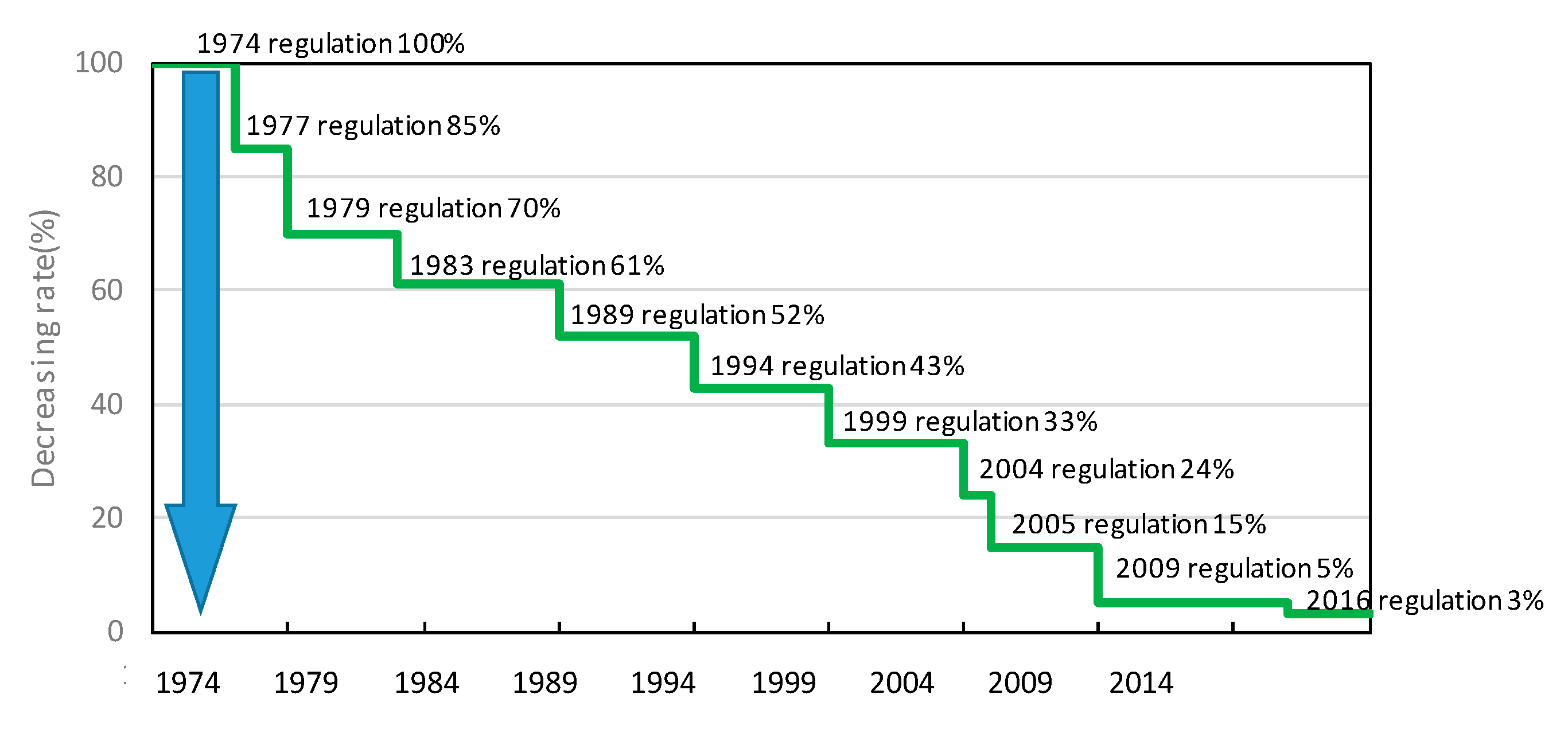
Emissions of NOx and VOCs reduced dramatically, and their environmental concentrations were also gradually decreasing. NOx emissions from stationary sources declined in a linear fashion due to such factors as the comprehensive total emissions control scheme conducted by the government of Kawasaki City. Emissions from motor vehicles also decreased substantially, and since 2003, when restrictions on the operation of diesel vehicles were imposed, the rate of decrease has been especially marked. The drop in NO has been especially conspicuous, resulting in a substantial change in the ratio of NO to NO2. The large fall in NO has probably been a factor in the significant drop in emissions from motor vehicles. As a result, the ratio of NO2 in the NOx emitted from motor vehicles in Kawasaki increased from 0.1 to 0.3 from FY2004 to FY2019, though its ratio had remained around 0.1 until FY2000. Both emissions and environmental concentrations of NMHC declined monotonously, but in recent years, the rate of decline in NOx concentrations has outstripped the rate of decline in NMHC concentrations. Until around 2005, the NMHC/NOx (ppmC/ppm) ratio remained in the vicinity of 5.5, but from 2005, it showed a rising trend such that by 2019, it had reached around 6.5.
(3)
The amount of generated Ox is another important indicator. Methods to estimate the amount of generated Ox during the daytime were introduced. This attempt was developed into DPOx as a new indicator for assessing the effectiveness of countermeasures for Ox reduction. This indicator involves deducting one day’s night concentration from the next day’s daytime concentration, allowing only the Ox generated in the area during the day to be assessed. The three-year moving average of the average DPOx during April to October exhibited a declining trend from FY2006, much like the new indicator from the MOE.

8. Discussion

The annual average concentration of Ox has been increasing in spite of the decrease in ambient NOx and VOCs since the 1990s. However, from the 2000s, a decrease in in situ photochemical production occurred in four metropolitan areas in Japan. It is expected that the reduction in NOx over a certain limit should bring further reduction in Ox, which will overcome the increase in Ox due to the reduction in NO titration [20]. Moreover, it has been shown that high Ox concentrations in Tokyo have fallen since the decline in NO2 after 2000 and the introduction of restrictions on VOC emissions in 2006 [18]. Because of these, a reduction in the three-year moving average of the averages of DPOx in Kawasaki for April–October from FY2006 was assumed to reflect a decrease in photochemical production in the city from around FY2006, because the declines in the NOx concentration and the NO2 concentration from the 2000s shown in Figure 18, the decline in the NMHC concentration shown in Figure 24, and the increase in NMHC/NOx shown in Figure 25 exceeded a certain limit. Therefore, it is supposed that DPOx may be a suitable indicator that reflects the impact of reductions in sources of NOx and VOCs in Kawasaki.
In light of the above, though meteorological conditions during the past 30 years have made it more likely for high concentrations of Ox to occur, it is considered that the amount of daily production of Ox has progressively decreased with reducing NOx and VOCs, which are Ox precursors, since FY2006. The same trend of reduction can also be shown in the number of PSW days and the new indicator from the MOE. However, because the new indicator from the MOE reflects zones with high Ox concentrations, it will also be affected by factors other than sources within the area, such as meteorological factors and transboundary transport of Ox. The effects of countermeasures for Ox control are thought to occur daily, not only on days of high concentration, but also on days of low concentration of Ox. Therefore, it is suggested that DPOx from April to October, as assessed based on the daytime production of Ox, is an indicator that reflects the impact of measures to reduce Ox precursors in sources within the area. Nevertheless, because this indicator could show unique tendencies due to sources being in close proximity in Kawasaki, we hope that analysis will be performed for various regions in which this indicator is being applied.

Author Contributions

This paper was written jointly by all the authors. S.W. designed the study and exercised overall supervisory control. A.F. analyzed the data on meteorology, NMHC, and relationships between Ox and its precursors involved in high Ox concentrations, while T.S. analyzed the data on NOx. K.F. contributed to the analysis of the Ox data and designed DPOx. D.Y. and S.I. edited the entire manuscript. All authors have read and agreed to the published version of the manuscript.

Funding

This research received no external funding.

Data Availability Statement

Publicly available datasets were analyzed in this study. This data can be found here: http://sc.city.kawasaki.jp/taiki/DOWNLOAD/YMSelectsk.html (accessed on 27 March 2021).

Acknowledgments

The data used in this paper were supplied from atmospheric constant-observation data for the past 30 years managed by Kawasaki Environment Research Institute (KERI). We also received advice from the Institute of Integrated Atmospheric Environment (IIAE) concerning administrative procedures for posting, which were carried out by KERI’s Takahiro Fukahori and Shiho Kasamatsu.

Conflicts of Interest

The authors declare no conflict of interest.

Appendix A. Kawasaki City Ordinance for Pollution Prevention

In Kawasaki, pollution problems in air and water from sooty smoke and dirty water emitted by factories emerged in the 1950s. In 1960, the Kawasaki city government implemented the Kawasaki City Ordinance for Pollution Prevention, but the pollution problems kept getting worse. The national government had established the Air Pollution Control Act in 1968, and the Kawasaki city government concluded pollution prevention agreements with large factories in Kawasaki between 1970 and 1972. In 1972, Kawasaki City became the first in Japan to implement a new ordinance introducing the total emissions approach, the Kawasaki City Ordinance for Pollution Prevention. The national government adopted the total emissions approach later, incorporating it into the Air Pollution Control Act.

Appendix B. A New Indicator from the MOE for Ox

The MOE proposed this indicator in 2016 to appropriately show the impact of Ox-related environmental improvements. It employed the averaged value over an 8 h period as this indicator rather than the averaged value over a 1 h period, which is employed as the EQS. This indicator is in line with standards from the WHO and the United States Environmental Protection Agency (US EPA).
The MOE assesses long-term trends in Ox concentrations using annual 99th percentile values of daily maximum eight-hour average concentrations, focusing on high-Ox-concentration zones problematic in Ox atmospheric pollution.

Appendix C. Emergency Measures Pursuant to the Air Pollution Control Act

In Japan, when the ambient Ox concentrations exceed a high level, the prefectural governor issues PSW pursuant to the Air Pollution Control Act. In Kawasaki, the governor of Kanagawa Prefecture issues PSW when the ambient Ox concentrations exceed 0.12 ppm at any one of the nine General sta. and are expected to remain high. When PSW are issued in Kawasaki, the governor of Kanagawa Prefecture informs residents in accordance with Kanagawa prefectural guidelines for emergency measures relating to air pollution and may issue a recommendation that business operators that emit large quantities of sooty smoke take measures to reduce emissions and endeavor to curtail VOC emissions and so on in the period from April to October.

Appendix D. Comprehensive Total Emissions Control Scheme

As a countermeasure to suspended particulate matter (SPM), in 2000, the Kawasaki city government incorporated comprehensive regulation for total pollution loads of SPM to major stationary sources into the Kawasaki City Ordinance for Conservation of Living Environment including Pollution Prevention, which replaced the Kawasaki City Ordinance for Pollution Prevention.
In this regulation, in addition to primary particles emitted directly from stationary sources, gaseous substances of SOx, NOx, and hydrogen chloride are converted to secondary particles by using certain coefficients, resulting in emissions as secondary particles, considering secondary formation of SPM. In this way, the total amount of primary particles and secondary particles are controlled.

Appendix E. Regulations for Motor Vehicles

The new motor vehicle exhaust emission regulations in Japan have been enforced since the year 1966, when the concentration of carbon monoxide from motor vehicles began to be controlled for the first time. Since then, substances to be controlled are being added continually to the list. Currently, carbon monoxide, NMHC, NOx, and PM are regulated. These regulations have been strengthened stepwise. A timeline of NOx regulations for heavy diesel vehicle exhaust is shown in Figure A1.
Figure A1. Timeline of NOx regulations for heavy diesel vehicles.
Atmosphere 12 00446 g0a1
Two types of regulations were applied to reduce emissions from in-use motor vehicles in the 1990s and in the early 2000s.
One of those, called the automobile NOx and PM law, sets emissions parameters in large metropolitan areas, which include Kawasaki, that had been significantly affected by these pollutants in the 1990s. It applies to commercial cargo vehicles (trucks, vans, and buses) and diesel passenger cars. If the vehicles cannot conform with emission parameters, their use is restricted as, for example, such vehicles cannot undergo inspection in the areas.
Another of the regulations is called the Tokyo Retrofit Program. The Tokyo government and several neighboring prefectures adopted diesel emission regulations, which required retrofitting of older in-use diesel vehicles with particle matter (PM) control devices (catalytic converters or particulate filters) or else replacing them with newer, cleaner models. The Tokyo retrofit requirements became effective in October 2003.

Appendix F. The Best-Mix Approach to Curbing VOC Emissions

The Japanese government established in 2004 a scheme based on a mix of regulatory and voluntary approaches to reduce emissions of VOCs, calling it a best mix. It aimed to reduce VOCs by 30% by 2010 from the 2000 level by using both direct regulations (10%) and voluntary efforts (20%). As a result, in FY2010, a nationwide reduction of 45% was achieved.

References

  1. Acid Deposition and Oxidant Research Center. Tropospheric Ozone a Growing Threat; Acid Deposition and Oxidant Research Centre: Niigata, Japan, 2006; Available online: https://www.acap.asia/wp-content/uploads/Ozone.pdf (accessed on 3 February 2021).
  2. National Research Council. Ozone-Forming Potential of Reformulated Gasoline; National Academy Press: Washington, DC, USA, 1999. [Google Scholar]
  3. Ho, W.C.; Hartley, W.R.; Myers, L.; Lin, M.H.; Lin, Y.S.; Lien, C.H.; Lin, R.S. Air Pollution, Weather, and Associated Risk Factors Related to Asthma Prevalence and Attack Rate. Environ. Res. 2007, 104, 402–409. [Google Scholar] [CrossRef]
  4. Watanabe, M.; Matsuo, N.; Yamaguchi, M.; Matsumura, H.; Kohno, Y.; Izuta, T. Risk assessment of ozone impact on the carbon absorption of Japanese representative conifers. Eur. J. For. Res. 2009, 129, 421–430. [Google Scholar] [CrossRef] [Green Version]
  5. Varotsos, C.; Tzanis, C.; Cracknell, A. The enhanced deterioration of the cultural heritage monuments due to air pollution. Environ. Sci. Pollut. Res. 2009, 16, 590–592. [Google Scholar] [CrossRef]
  6. Varotsos, C.; Cartalis, C. Re-evaluation of surface ozone over Athens, Greece, for the period 1901–1940. Atmos. Res. 1991, 26, 303–310. [Google Scholar] [CrossRef]
  7. Varotsos, C.; Efstathiou, M.N.; Kondratyev, K.Y. Long-term variation in surface ozone and its precursors in Athens, Greece: A forecasting tool. Environ. Sci. Pollut. Res. 2003, 10, 19–23. [Google Scholar]
  8. Varotsos, C.; Ondov, J.M.; Efstathiou, M.N.; Cracknell, A.P. The local and regional atmospheric oxidants at Athens (Greece). Environ. Sci. Pollut. Res. 2014, 21, 4430–4440. [Google Scholar] [CrossRef]
  9. Wakamatsu, S.; Ohara, T.; Uno, I. Recent trend in precursor concentrations and oxidant distribution in the Tokyo and Osaka areas. Atmos. Environ. 1996, 30, 715–721. [Google Scholar] [CrossRef]
  10. Wakamatsu, S.; Schere, K.L. A Study Using a Three Dimensional Photochemical Smog Formation Model Under Conditions of Complex Flow: Application of the Urban Air shed Model to the Tokyo Metropolitan Area; US-EPA Report; EPA/600/3-91/015; Environmental Protection Agency: Research Triangle Park, NC, USA, 1991; pp. 1–84.
  11. Wakamatsu, S.; Uno, I.; Ohara, T.; Schere, K.L. A study of the relationship between photochemical ozone and its precursor emissions of nitrogen oxides and hydrocarbons in the Tokyo area. Atmos. Environ. 1999, 33, 3097–3108. [Google Scholar] [CrossRef]
  12. Kitayama, K.; Morino, Y.; Yamaji, K.; Chatani, S. Uncertainties in O3 concentrations simulated by CMAQ over Japan using four chemical mechanisms. Atmos. Environ. 2019, 198, 448–462. [Google Scholar] [CrossRef]
  13. Chatani, S.; Yamaji, K.; Itahashi, S.; Saito, M.; Takigawa, M.; Morikawa, T.; Kanda, I.; Miya, Y.; Komatsu, H.; Sakurai, T.; et al. Identifying key factors influencing model performance one ground-level ozone over urban areas in Japan through model inter-comparisons. Atmos. Environ. 2020, 223. [Google Scholar]
  14. Chatani, S.; Shimadera, H.; Itahashi, S.; Yamaji, K. Comprehensive analyses of source sensitivities and apportionments of PM2.5 and ozone over Japan via multiple numerical techniques. Atmos. Chem. Phys. 2020, 20, 10311–10329. [Google Scholar] [CrossRef]
  15. Sather, M.E.; Cavender, K. Trends analysis of 30 years of ambient 8 hour ozone and precursor monitoring data in the south central U.S: Progress and challenges. Environ. Sci. 2016, 18, 819–831. [Google Scholar]
  16. Gao, W.; Tie, X.; Xu, J.; Huang, R.; Mao, X.; Zhou, G.; Chang, L. Long-term trend of O3 in a mega City (Shanghai), China: Characteristics, causes, and interactions with precursors. Sci. Total Environ. 2017, 603, 425–433. [Google Scholar] [CrossRef]
  17. Ministry of Environment, Japan. On Situation of Air Pollution in FY Heisei 30. 2020. Available online: https://www.env.go.jp/air/osen/jokyo_h30/index.html (accessed on 7 January 2021). (In Japanese)
  18. Wakamatsu, S.; Morikawa, T.; Ito, A. Air pollution trends in Japan between 1970 and 2012 and impact of urban air pollution countermeasures. Asian J. Atmos. Environ. 2013, 7, 177–190. [Google Scholar] [CrossRef] [Green Version]
  19. Itano, Y.; Wakamatsu, S.; Hasegawa, S.; Kobayashi, S. Local and regional contributions to springtime ozone in the Osaka metropolitan area, estimated from aircraft observations. Atmos. Environ. 2005, 40, 2117–2127. [Google Scholar] [CrossRef]
  20. Akimoto, H.; Mori, Y.; Sasaki, K.; Nakanishi, H.; Ohizumi, T.; Itano, Y. Analysis of ground-level ozone on Japan for long-term trend during 1990–2010: Causes of temporal and spatial variation. Atmos. Environ. 2015, 102, 302–310. [Google Scholar] [CrossRef]
  21. Ministry of Environment, Japan. On Situation of Air Pollution in FY Heisei 26. 2015. Available online: https://www.env.go.jp/air/osen/jokyo_h26/index.html (accessed on 7 January 2021). (In Japanese)
  22. Japan Meteorological Agency, Japan. Extreme Weather in Japan in the Summer of 2013—Summary of Analytical Findings from the Investigative Commission for Abnormal Weather Phenomena. Available online: http://www.jma.go.jp/jma/press/1309/02d/extreme20130902.pdf (accessed on 7 January 2021). (In Japanese)
  23. Kubo, T.; Iino, H.; Yamamoto, K.; Nakatsubo, R.; Takimoto, M.; Takaishi, Y. Analysis of severe ozone pollution during 24–26 May 2019 over Hyogo Prefecture. Bull. Hyogo Pref. Inst. Environ. Sci. 2019, 10, 12–18. (In Japanese) [Google Scholar]
  24. Kimura, F.; Shiihashi, M. Application of quasi-stational reactive diffusion model to long-term average concentration. J. Jpn. Soc. Air Pollut. 1988, 23, 41–51, (In Japanese with English abstract and figure captions). [Google Scholar]
  25. Wakamatsu, S.; Uno, I.; Suyama, Y.; Asou, T.; Makino, H. Observational study of air pollutants distribution using airship. J. Jpn. Soc. Air Pollut. 1990, 25, 97–101, (In Japanese with English abstract and figure captions). [Google Scholar]
  26. Tran, T.N.T.; Goto, D.; Yashiro, H.; Murata, R.; Sudo, K.; Tomita, H.; Satoh, M.; Nakajima, T. Evaluation of summertime surface ozone in Kanto area of Japan using a semi-regional model and observation. Atmos. Environ. 2017, 153, 163–181. [Google Scholar]
  27. Khiem, M.; Ooka, R.; Huang, H.; Hayami, H.; Yoshikado, H.; Kawamoto, Y. Analysis of the Relationship between Changes in Meteorological Conditions and the Variation in Summer Ozone Levels over the Central Kanto Area. Adv. Meteorol. 2010, 1–13. [Google Scholar] [CrossRef] [Green Version]
  28. Kiriyama, Y.; Shimadera, H.; Itahashi, S.; Hayami, H.; Miura, K. Evaluation of the Effect of Regional Pollutants and Residual Ozone on Ozone Concentrations in the Morning in the Inland of the Kanto Region. Asian J. Atmos. Environ. 2015, 9, 1–11. [Google Scholar] [CrossRef] [Green Version]
  29. Ookaa, R.; Khiemb, M.; Hayamic, H.; Yoshikado, H.; Huange, H.; Kawamotoa, Y. Influence of meteorological conditions on summer ozone levels in the central Kanto area of Japan. Procedia Environ. Sci. 2011, 4, 138–150. [Google Scholar] [CrossRef] [Green Version]
Figure 1. Location of Kawasaki City in Japan.
Atmosphere 12 00446 g001
Figure 2. Locations of air quality monitoring stations in Kawasaki. In the figure, General sta. are denoted as ● and Roadside sta. are denoted as ▲.
Atmosphere 12 00446 g002
Figure 3. Trends in the annual averages of Ox. Ox (All the time): annual averages of hourly Ox for all nine General sta. Ox (Daytime): annual averages of hourly Ox for all nine General sta. from 6 a.m. to 8 p.m. Ox (Night): annual averages of hourly Ox for all nine General sta. from 12 a.m. to 5 a.m. and 9 p.m.–12 a.m.
Atmosphere 12 00446 g003
Figure 4. Trend in monthly average Ox for each month. Ox: monthly averages of hourly Ox at all nine General sta.
Atmosphere 12 00446 g004
Figure 5. Rate of increase in monthly average Ox concentrations for each month. Ox concentrations: same as Figure 4. Rate of increase: slope of linear regression line for monthly averages for each decade.
Atmosphere 12 00446 g005
Figure 6. Trend in the number of days on which photochemical smog warnings (PSW) were issued in Kawasaki.
Atmosphere 12 00446 g006
Figure 7. Trend in the three-year moving average for daily maximum of Ox concentrations. Ox: daily maximum of hourly Ox at all nine General sta.
Atmosphere 12 00446 g007
Figure 8. Trend in a new indicator from the Ministry of the Environment (MOE) (three-year moving average of the annual 99th percentile of the daily maximum for the eight-hour value). Ox concentration: calculation of annual 99th percentile of the daily maximum for the eight-hour value.
Atmosphere 12 00446 g008
Figure 9. Trend in annual averages of air temperature. Air temperature: annual averages of daily maximum, daily average, and daily minimum of air temperature at all nine General sta.
Atmosphere 12 00446 g009
Figure 10. Rate of increase over time in monthly averages of air temperature (1990−2019). Air temperature: same as Figure 9. Rate of increase in air temperature: slope of linear regression line for the monthly average temperature for each month over 30 years.
Atmosphere 12 00446 g010
Figure 11. Trend in annual averages of wind speed. Wind speed: annual averages of hourly wind speed at six General sta. (Daishi, Nakahara, Takatsu, Miyamae, Tama, and Asao).
Atmosphere 12 00446 g011
Figure 12. Rate of increase over time in the monthly averages of wind speed for each month (1990−2019). Wind speed: same as Figure 11. Rate of increase in wind speed: slope of linear regression line for the monthly average temperature for each month over 30 years.
Atmosphere 12 00446 g012
Figure 13. Trends in annual averages of solar radiation compared with those of air temperature. Solar radiation: annual averages of daily total amount of solar radiation at two General Sta. (Tajima from 1990–2006; Tajima and Saiwai from 2007 to 2019). Air temperature: same as Figure 9.
Atmosphere 12 00446 g013
Figure 14. Rate of increase over time in the monthly average of solar radiation for each month. Solar radiation: same as Figure 13. Rate of increase in solar radiation: slope of linear regression line for the monthly average for each month over 30 years.
Atmosphere 12 00446 g014
Figure 15. Trend in the emissions of NOx from factories and workplaces. NOx emissions: reported figures for annual NOx emissions from factories and workplaces with facilities that emit soot and smoke, as specified by the Air Pollution Control Act.
Atmosphere 12 00446 g015
Figure 16. Trend in the emissions of NOx from motor vehicles. NOx emissions: estimates from the Kawasaki city government.
Atmosphere 12 00446 g016
Figure 17. Trends in the annual averages of NOx, NO, and NO2. NOx, NO2, and NO: annual averages of hourly NOx, NO2, and NO at all nine General sta. and all nine Roadside sta.
Atmosphere 12 00446 g017
Figure 18. Trends in the annual averages of NO2/NOx. NO2, NOx: same as Figure 17.
Atmosphere 12 00446 g018
Figure 19. Trend in NOx, NO, and NO2 over time at night during the cold season. NOx, NO, and NO2: annual averages of hourly NOx, NO, and NO2 at nine General sta. and nine Roadside sta. in the cold season.
Atmosphere 12 00446 g019
Figure 20. Trend in the average of NOx, NO2, and NO at Roadside sta. in the nighttime during the cold season. NOx, NO2, and NO: same as Figure 19.
Atmosphere 12 00446 g020
Figure 21. Trends in the average of NO2/NOx at Roadside sta. less that at General sta. at night during the cold season. NOx and NO2: same as Figure 19.
Atmosphere 12 00446 g021
Figure 22. Trend in volatile organic compound (VOC) emissions from stationary sources in Kanagawa Prefecture (estimated based on the VOC inventory report from the MOE).
Atmosphere 12 00446 g022
Figure 23. Trend in the annual averages of non-methane hydrocarbons (NMHC). Average of 3 h: annual averages of 3 h average of NMHC from 6 a.m. to 9 a.m. at seven General sta. (Daishi, Tajima, Kawasaki, Saiwai, Nakahara, Takatsu, and Tama). Average of 24 h: annual averages of 24 h average of NMHC concentrations from 12 a.m. to 12 a.m. at seven General sta.
Atmosphere 12 00446 g023
Figure 24. Trend in the annual averages of NMHC/NOx. NMHC: same as Figure 23. NOx: annual averages of three-hour average of NOx from 6 a.m. to 9 a.m. at seven stations; same as Figure 23.
Atmosphere 12 00446 g024
Figure 25. Relationship between Ox, NOx, and NMHC. Ox: annual averages of daily maximum of Ox at all nine General sta. NOx: annual averages of three-hour average of NOx from 6 a.m. to 9 a.m. at all nine General sta. NMHC: same as Figure 23.
Atmosphere 12 00446 g025
Figure 26. Number of days in patterns A, B, and C and trend over time in Ox. Selection conditions: A meets (1); B meets (1) and (2); and C meets (1), (2), and (3). Ox average of the past three years: This is the three-year moving average of the figure averaged for the number of extracted days of the average for all nine General sta. of the daily high of extracted-day hourly values. For example, the figure for 2007 is expressed as the three-year average for 2005–2007. Ox: figure averaged for the number of extracted days of the average for all nine General sta. of the daily high of extracted-day hourly values.
Atmosphere 12 00446 g026
Figure 27. Relationship between Ox, NOx, and NMHC on extracted days. Ox: figure averaged for the number of extracted days of the average for all nine General sta. of the daily maximum of extracted-day hourly values. NOx: figure averaged for the number of extracted days of the average for all nine General sta. of the extracted-day three-hour average from 6 a.m. to 9 a.m. NMHC: figure averaged for the number of extracted days of the average for seven General sta. of the extracted-day three-hour average from 6 a.m. to 9 a.m. Days: number of extracted days.
Atmosphere 12 00446 g027
Figure 28. Relationship between NMHC and NOx all the year round and on extracted days. NMHC concentration: average for seven General sta. of three-hour average from 6 a.m. to 9 a.m. NOx concentration: average for all nine General sta. of three-hour average from 6 a.m. to 9 a.m. All year: annual average. Pattern C days: annual average on extracted days.
Atmosphere 12 00446 g028
Figure 29. An image of the daytime production of photochemical oxidant (DPOx). Ox: averaged hourly Ox at all General sta. Time: the period from 9 p.m. on 31 July to 12 a.m. on 2 August in 2019.
Atmosphere 12 00446 g029
Figure 30. Trend in three-year moving averages of DPOx from April to October. Note: If the daytime Ox concentrations are lower than the previous day’s nighttime Ox concentrations, the day’s DPOx is zero, and the day’s DPOx is included in the averaged DPOx. Note: If the total number of hours with no measurement data is over 5 between the one day’s 9 p.m. and the next day’s 8 p.m., the day’s DPOx is excluded from averaged DPOx.
Atmosphere 12 00446 g030
Figure 31. Trends in NOx and NMHC from April to October. (a) NOx: annual averages of hourly NOx for all nine General sta. from April to October. (b) NMHC: annual averages of hourly NMHC for seven General sta. from April to October.
Atmosphere 12 00446 g031
Figure 32. Trend in DPOx with the new indicator from the MOE. DPOx: same as Figure 31. New indicator from the MOE: same as Figure 8.
Atmosphere 12 00446 g032
Table 1. Environmental quality standard (EQS) for photochemical oxidants (Ox) in Japan (established in 1973).
Environmental quality standardHourly value should not exceed 0.06 ppm
(118 μg/m3).
Evaluation methods of environmental quality standardIf the one-hour mean value exceeds 0.06 ppm, it is judged not to have achieved the standard.
Table 2. Meteorological selection conditions.
Conditions
(1)Day on which the average *1 daily maximum air temperature was 30 °C or higher
(2)Day on which the average *1 daily maximum wind speed was 3 m/s or lower
(3)Day on which the average *2 daily total solar radiation exceeded 10 MJ/m2
*1 Average for all nine General sta. *2 Average for two stations Tajima and Saiwai (however, figures for 1990–2006 are for Tajima only).
Publisher’s Note: MDPI stays neutral with regard to jurisdictional claims in published maps and institutional affiliations.

