Contribution of Local and Transboundary Air Pollution to the Urban Air Quality of Fukuoka, Japan

Abstract

Transboundary air pollution (TAP) and local air pollution (LAP) influence the air quality of urban areas. Fukuoka, located on the west side of Japan and affected by TAP from the Asian continent, is a unique example for understanding the contribution of LAP and TAP. Gaseous species and particulate matter (PM) were measured for approximately three weeks in Fukuoka in the winter of 2018. We classified two distinctive periods, LAP and TAP, based on wind speed. The classification was supported by variations in the concentration of gaseous species and by backward trajectories. Most air pollutants, including NOx and PM, were high in the LAP period and low in the TAP period. However, ozone was the exception. Therefore, our findings suggest that reducing local emissions is necessary. Ozone was higher in the TAP period, and the variation in ozone concentration was relatively small, indicating that ozone was produced outside of the city and transported to Fukuoka. Thus, air pollutants must also be reduced at a regional scale, including in China.

1. Introduction

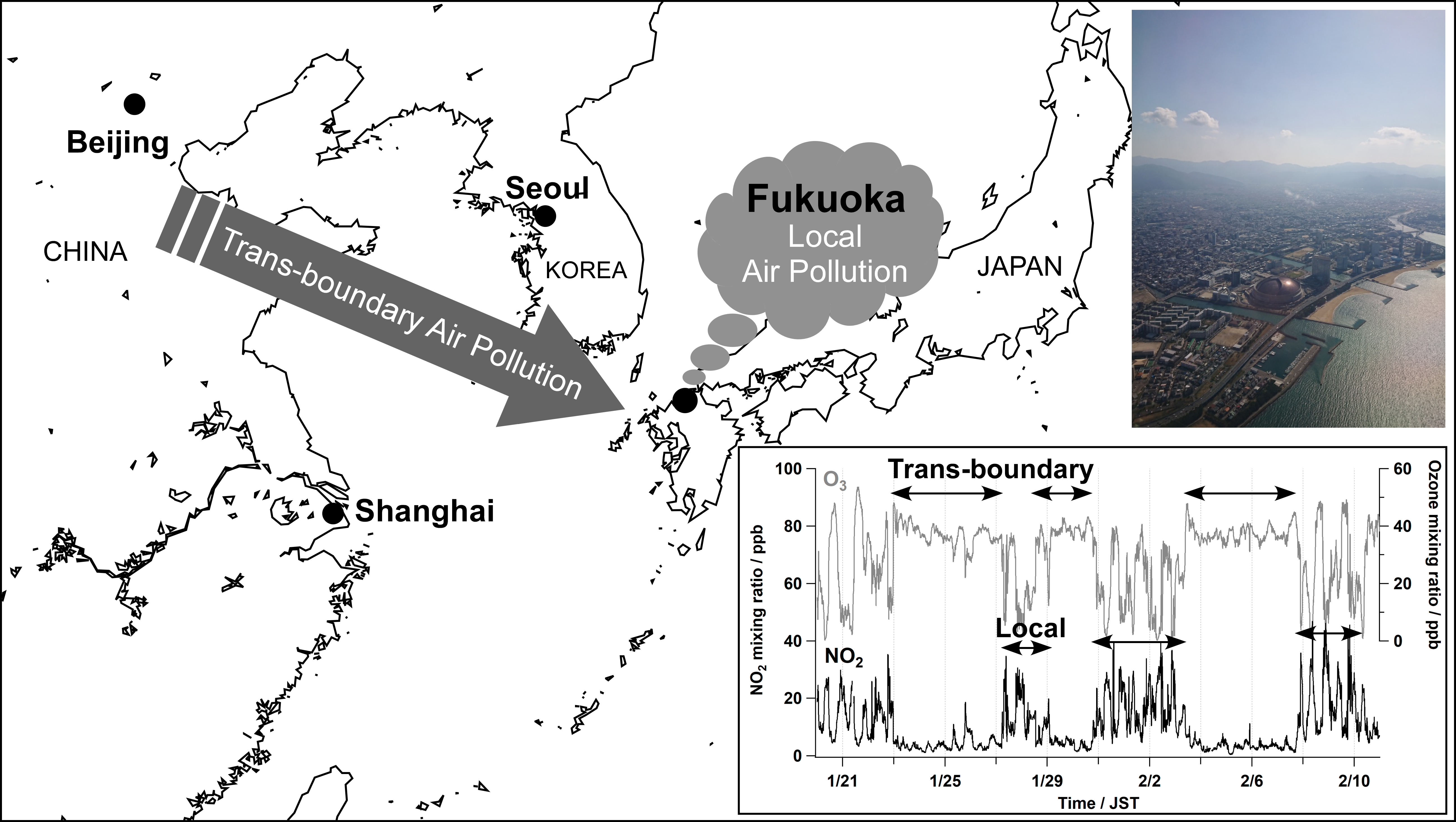
Urban populations are growing, and many people are exposed to air pollution in living and working areas. Air quality in urban areas is important because air pollution affects human health [1]. Urban air quality is often determined by local air pollution (LAP) emitted from the city itself, but is also affected by transboundary air pollution (TAP), depending on the location of the city. For example, the air quality in the western region of Japan is affected by TAP because Japan is located on the leeward side of the Asian continent. Continental pollutants are transported to Japan by the seasonal monsoon [2,3,4,5,6,7] (references therein).

Fukuoka, one of the largest cities in Japan, has approximately 1.5 million residents and many vehicles, commercial areas, and industrial areas. Therefore, local emissions are expected to be large, and the air quality in Fukuoka is considered to be largely determined by LAP. Additionally, air quality in Fukuoka is often affected by TAP because Fukuoka is located on the western side of Japan [4,7,8]. In this context, Fukuoka is in a unique location that results in the air quality being affected by LAP and TAP. Thus, understanding the contributions of both LAP and TAP is essential to improve the air quality in Fukuoka.

The air quality in Japan has improved in recent years. Based on a report from the Ministry of Environment Japan in 2018 [9], the achievement rate of the Japan Environmental Standard for fine particulate matter (PM_2.5) recently increased from 30–40% from 2010–2014 to over 80% in 2017. One primary reason for this change is the continuous effort to reduce emissions in Japan [10]. Another reason is the decrease in emissions in China. Since 2013, the Chinese government has been taking measures to mitigate air pollution. Consequently, SO₂ and NOx emissions in China decreased, and the annual mean of PM_2.5 concentrations in major Chinese cities decreased from 72 μg m⁻³ in 2013 to 39 μg m⁻³ in 2017 [9]. The PM_2.5 concentration in Fukuoka has decreased proportionally relative to the decrease in emissions in China [6], indicating that LAP and TAP are important for air quality in Fukuoka.

Although the PM_2.5 concentration in Japan has recently decreased, oxidant (primarily ozone) concentrations have done the opposite [9]. In May 2007, a high ozone event was observed that was caused by TAP from China [11]. Based on the analysis of long-term data between 1985 and 2005, Nagashima et al. [12] reported that approximately 35% of ozone came from China. Recently, Chatani et al. [8] investigated the contribution of ozone from outside Japan using sensitivity and source apportion methods. Their analysis showed that most of the ozone was transported from China, even after the Chinese government imposed stringent emission controls.

We have studied the Fukuoka air quality from a TAP point of view [4,6,7]. However, we need to consider LAP and TAP, because emissions in China have recently been greatly reduced [9]. In this study, we measured gaseous species and particulate matter (PM) in Fukuoka City in the winter of 2018. We analyzed diurnal variations in gas and PM concentrations with the meteorological conditions to understand the contribution of LAP and TAP to air quality in Fukuoka.

2. Materials and Methods

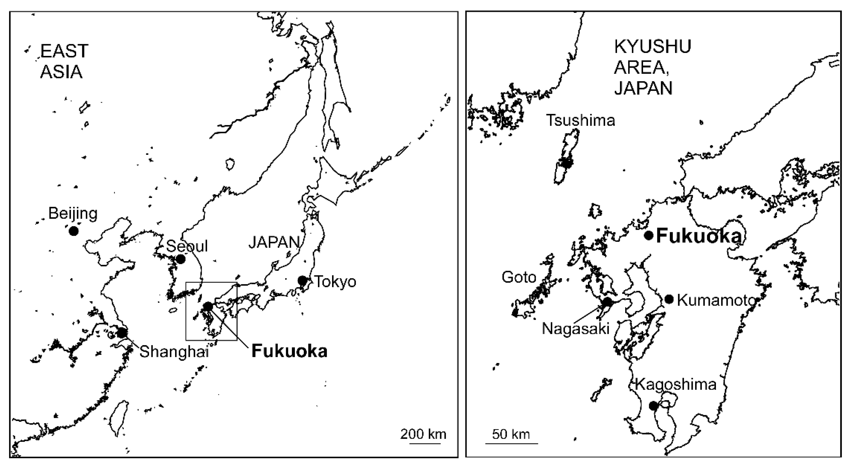
The measurements were conducted at the 18th building of Fukuoka University (Fukuoka Prefecture, 33.55° N 130.36° E). Figure 1 shows the location of Fukuoka City. The university is located in a residential area, approximately 5 km from a commercial area, and the building is several hundred meters from the metropolitan highway.

The instruments were set in the laboratory on the fourth floor of the 18th building at a height of approximately 15 m. The inlet for both gaseous species and PM was separately projected from the windows. Teflon tubes were used for the gaseous species, and stainless tubes were used for PM. The laboratory was air-conditioned, and the room temperature was maintained at approximately 20 °C during the observation period [4]. The measurement period was from 20 January to 10 February, 2018.

Gaseous species were measured using an ozone monitor (Thermo 49 i/J), CO monitor (Thermo 48iTLE), NOx monitor (Horiba APNA-370), and SO₂ monitor (Horiba APSA-370). O₃ was measured by UV absorption, CO by nondispersive infrared spectroscopy, NOx by chemiluminescence, and SO₂ by pulsed UV-fluorescence [13]. The zero and span concentrations of CO were periodically checked using zero gas and span gas. A zero gas (CO-free air) was generated in the CO monitor which was equipped with a zero-gas generator. A span gas of 1 ppm was injected from the gas cylinder (Taiyo Nippon Sanso Co. Ltd., Tokyo, Japan).

The particle number concentration (PN) was measured using a scanning mobility particle sizer (SMPS 3034, TSI, Shoreview, MN, USA) [13]. The measured range of the particle diameter (D_p) was 10–500 nm. The PM chemical composition was measured using a quadrupole-type aerosol mass spectrometer (Q-AMS, Aerodyne Research Inc., Billerica, MA, USA) which can measure sulfate, nitrate, ammonium ions, and organics for fine particles (PM₁). The aerodynamic lens of Q-AMS separates gases and aerosols to form a particle beam, which targets the heated vaporizer at 873 K (600 °C), where nonrefractory species of PM are vaporized. The vaporized molecules were ionized with a 70 eV electron impactor, and the ions were analyzed using a quadrupole type mass spectrometer. Calibration was performed using ammonium nitrate (NH₄NO₃) particles with a D_p of 350 nm. The collection efficiency was set at 1.0. Inorganic species, such as sulfate and nitrate, were calculated from the mass signals. Organics were calculated by subtracting the known inorganic and gaseous species from the total mass [2,4,14,15]. The black carbon (BC) concentration in the PM_2.5 particles was measured using an Aethalometer (AE-16, Magee Scientific, Berkeley, CA, USA), with an instrumental optical absorption cross-section of 16.6 m² g⁻¹ at a wavelength of 880 nm. The optical attenuation of the aerosol-loaded filter tape was recorded at 15 min intervals, which defined the time resolution of the BC measurement [16]. Airflow introduced to the Aethalometer was first passed through a sharp-cut cyclone separator (SCC1.829, BGI, Butler, NJ, USA) to remove particles with an aerodynamic diameter greater than 2.5 μm.

The meteorological data for wind direction, wind speed, temperature, relative humidity, pressure, and precipitation were measured using a meteorological monitor (WXT520, Vaisala, Helsinki, Finland) which was set on the roof of the 18th building of Fukuoka University.

A mass concentration of PM_2.5 was obtained from the Kashii monitoring station which was operated by the Fukuoka Institute of Health and Environmental Sciences. The direct solar radiation data measured at the Fukuoka Meteorological Office (33.58° N, 130.38° E) were obtained from the Japan Meteorological Agency.

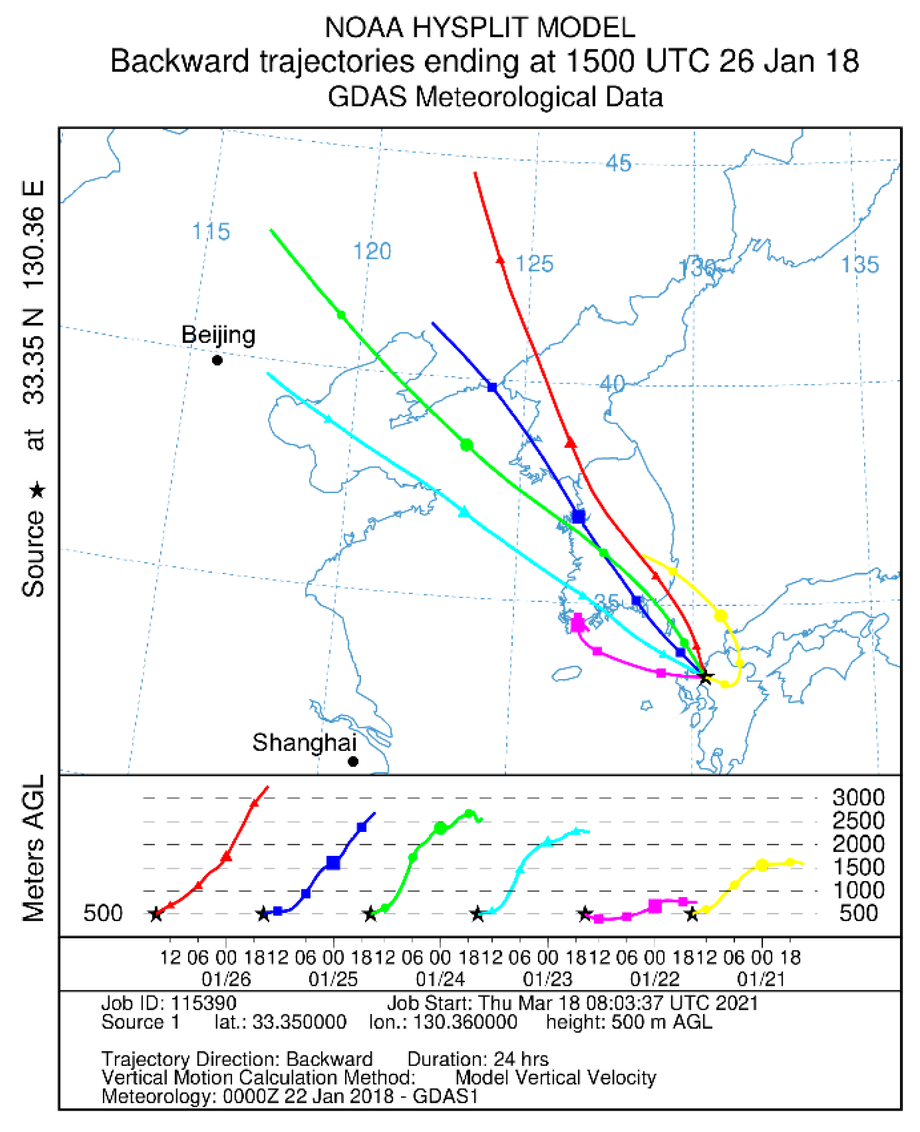
Backward trajectories (BT) were calculated using the vertical motion mode of the Hybrid Single-Particle Lagrangian Integrated Trajectory (HYSPLIT) model and the Global Data Assimilation System meteorological dataset [17,18]. Trajectories started at an altitude of 500 m, and the BT was calculated for 72 h. A positive matrix factorization (PMF) analysis was applied to the mass spectra of organics which was originally developed by Paatero and Tapper [19] and Paatero [20], and a customized evaluation tool (version 2.04) for AMS was developed by Ulbrich et al. [21]. The interpretations in the current study followed previous results [22,23,24].

3. Results

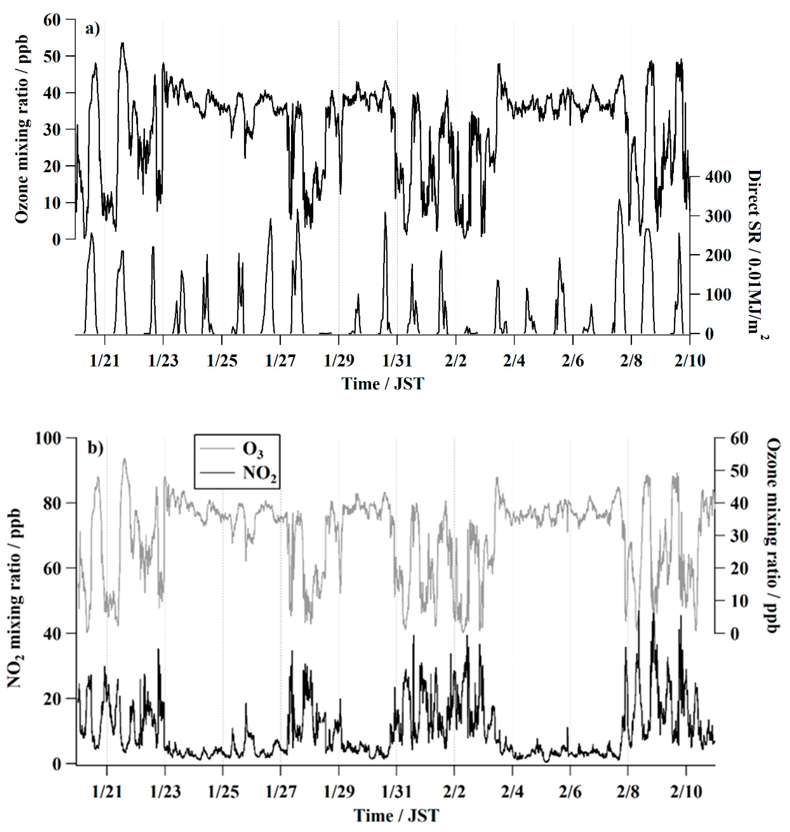
Figure 2a shows the ozone concentration (mixing ratio) and the direct solar radiation. Ozone showed diurnal variation and was high during the day and low in the morning and at night from 20–22 January, 27–28 January, 31 January to 2 February, and 8–10 February. During the same periods, the diurnal variation of ozone corresponded to direct solar radiation, indicating that ozone was primarily produced by photochemical processes. From 23–26 January, 29–30 January, and 3–7 February, the ozone concentration variation was relatively small (approximately 40 ppb), but the direct solar radiation showed diurnal variation, indicating that the ozone concentration was determined by factors other than photochemical processes. We considered that ozone was produced outside of the city and was transported to Fukuoka over a long distance. The concentrations (mixing ratios) of NO₂ and ozone are shown in Figure 2b. Ozone and NO₂, for example, show an anticorrelation from 20–22 January, indicating that titration occurred between ozone and NO to produce NO₂, as chain reactions occur under solar radiation. From 23–26 January, 29–30 January, and 3–7 February, the NO₂ concentration was low, and the variation was relatively small.

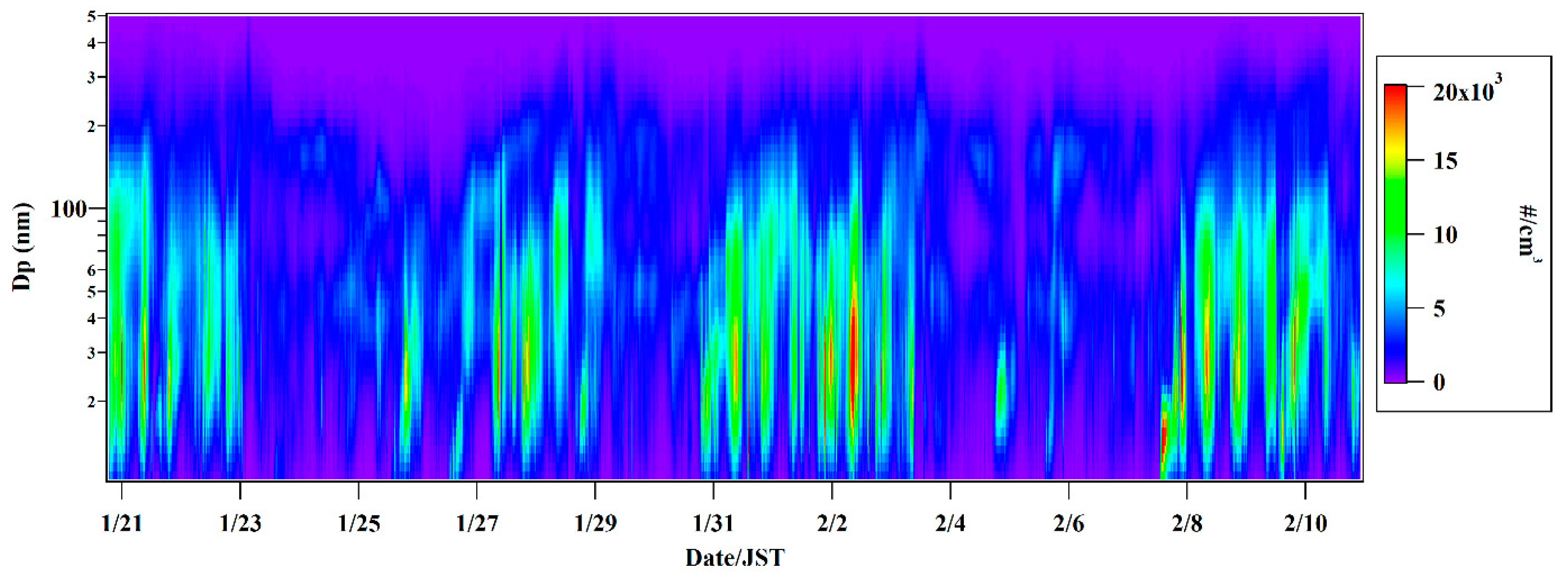
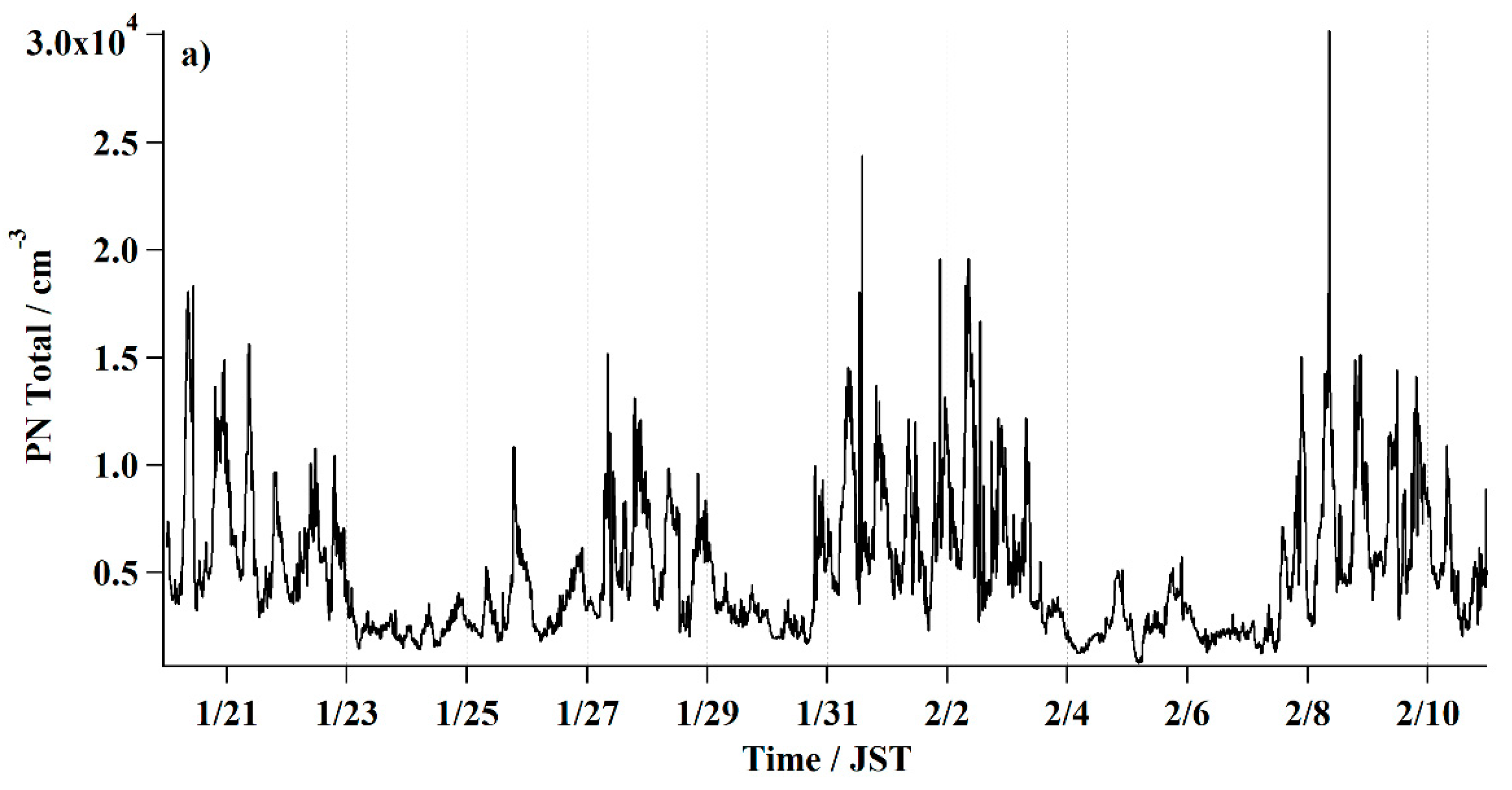
The PN of the diameter range from 10–500 nm is shown in Figure 3. The PN concentration of D_p < 200 nm periodically varied from low (approximately 300 cm⁻³) to high (15,000 cm⁻³) from 20–22 January, 27–28 January, 31 January to 2 February, and 8–10 February, which correspond to the periods when the ozone diurnal variation was observed. The total PN also showed a similar variation with ozone concentration, indicating that secondary particles were produced and grew into larger particles. 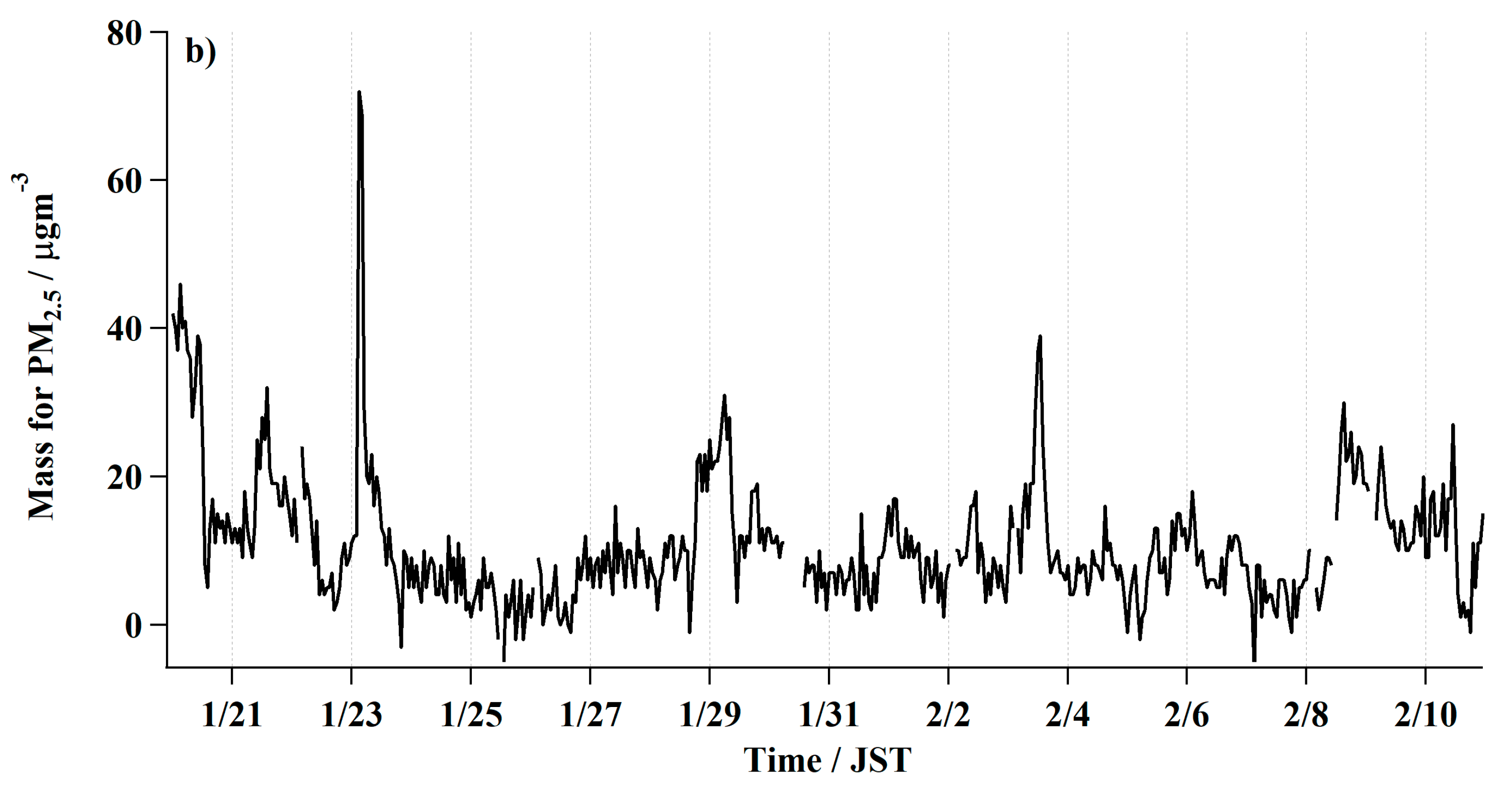Low PN concentrations were observed from 23–26 January, 29–30 January, and 3–7 February (Figure 4a). The low PN concentrations corresponded to periods in which the ozone concentration variation was relatively small (approximately 40 ppb). Figure 4b shows the mass concentration of PM_2.5 which, unlike the PN concentration, did not show a clear variation.

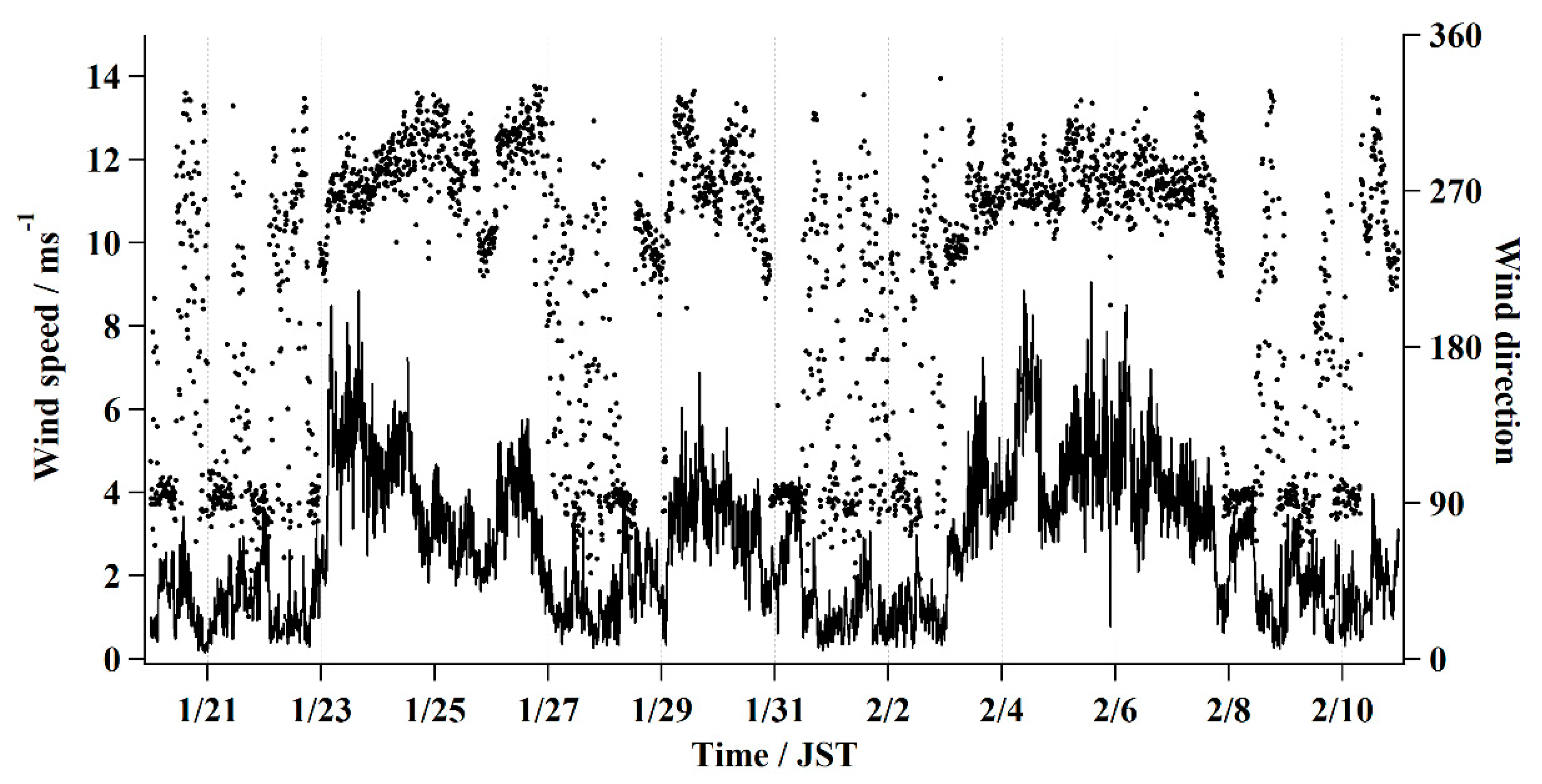
Figure 5 shows the wind speed and direction. The wind speed changed periodically. For example, the 10 min average was low from 20–22 January and high from 23–27 January. The wind direction also changed. Easterly and westerly winds were mixed from 20–22 January, whereas westerly winds were primarily observed from 23–27 January. The variation in wind speed corresponded to the variation in ozone concentration. At low wind speeds, ozone showed diurnal variation, whereas ozone showed relatively low variation at high wind speeds.

Based on the average wind speed and direction, we classified the observation periods into two groups:

(1)

Group A: Low wind speed (less than 3 ms⁻¹) varied wind direction.

(2)

Group B: High wind speed (more than 3 ms⁻¹) and primarily westerly wind direction.

Based on these criteria, we classified the days for Group A as 20–22 January, 27–28 January, 31 January to 2 February, and 8–10 February, and those in Group B as 23–26 January, 29–30 January, and 3–7 February. The classification into two groups was slightly rough, but worked relatively well to characterize the air pollution periods in Fukuoka (shown in the next section).

Table 1. Average values of gas, meteorological, and PM data for Groups A and B.

		Gas and Meteorological Data
Group		O3 /ppb	NO /ppb	NO2 /ppb	CO /ppm	SO2 /ppb	WS *3 /ms−1	Temp. *4 /°C	RH *5 /%
Group A	Average	23.5	3.03	15.3	0.32	1.24	1.50	5.13	65.4
(LAP *1)	S.D.	13.5	6.21	8.39	0.12	0.87	0.84	3.17	14.3
Group B	Average	36.4	0.56	4.60	0.23	1.02	3.90	1.62	51.6
(TAP *2)	S.D.	5.41	0.48	3.76	0.08	0.50	1.42	2.05	8.53
		PM Data
Group		Total Particle Number /cm−3	BC /ng m−3	PM2.5 /µg m−3	NO3− /µg m−3	SO42− /µg m−3	Fraction of Factor 1 /%	Fraction of Factor 2 /%
Group A	Average	6868	413	12.4	1.76	1.80	56.4	43.6
(LAP)	S.D.	3210	222	8.33	1.19	0.93	16.1	16.1
Group B	Average	3168	229	9.07	0.82	1.71	65.8	34.2
(TAP)	S.D.	1701	180	8.69	1.17	1.11	19.6	19.6

*1 LAP: local air pollution; *2 TAP: transboundary air pollution; *3 WS: wind speed; *4 Temp.: temperature; *5 RH: relative humidity.

shows the average values for the gas, PM, and meteorological data.

4. Discussion

4.1. Classification of Groups A and B

Based on the aforementioned results, we consider that Group A belongs to the LAP period, and Group B belongs to the TAP period. In the winter season, air masses are transported from Siberia with high altitude to Fukuoka as well as from the coastal region of China, which is typical transport of air pollution. In this study, these two cases were treated as TAP to distinguish from LAP, because the main objective of the classification was to separate the local air pollution from the pollution transported from outside.

A clear relationship was observed between the wind speed and the variation in ozone concentration. When the average wind speed was low in Group A (1.5 m s⁻¹), the ozone concentration showed diurnal variation, with an average concentration of 24 ppb (Table 1). When the average wind speed was high in Group B (3.9 ms⁻¹), the variation in ozone concentration was relatively small (Figure 2a), and ozone concentration was higher in Group B (36.4 ppb) than in Group A (23.5 ppb). The NO₂ concentration varied according to the ozone variation and was high in Group A (15.3 ppb) and low in Group B (4.60 ppb). Carbon monoxide (CO) showed a similar trend to NO₂; thus, CO was higher in Group A (0.32 ppm) than in Group B (0.23 ppm). These results indicate that Group A belonged to the LAP period, because local photochemical processes occurred under low wind speed conditions, leading to variations in ozone and NO₂ concentrations.

In contrast, Group B belonged to the TAP period. The ozone variation was relatively small, and NO₂ was low during the Group B period. Although local air pollution was common, the contribution of local photochemical processes was relatively small under higher wind speed conditions. To explain the relatively high ozone concentration in Group B, we considered that ozone was transported from outside the Fukuoka region. In Group B, the wind direction was westerly, and the air temperature was lower with lower relative humidity than that in Group A. The BT for 23–26 January (Figure 6) showed that the air masses were transported from the Asian continent, indicating that the seasonal monsoon from the continent to Japan prevailed during the Group B period, in which synoptic scale weather conditions controlled the transport of air pollutants. Therefore, Group B belonged to the TAP period.

4.2. PM Variation during the LAP and TAP Periods

A clear relationship was observed between wind speed and PN concentration. When the wind speed was low in Group A (LAP), the PN concentration was high (approximately 6900 cm⁻³). Conversely, when the wind speed was high in Group B (TAP), the PN concentration was low (approximately 3200 cm⁻³). Trends similar to those of the gaseous species were observed for PN.

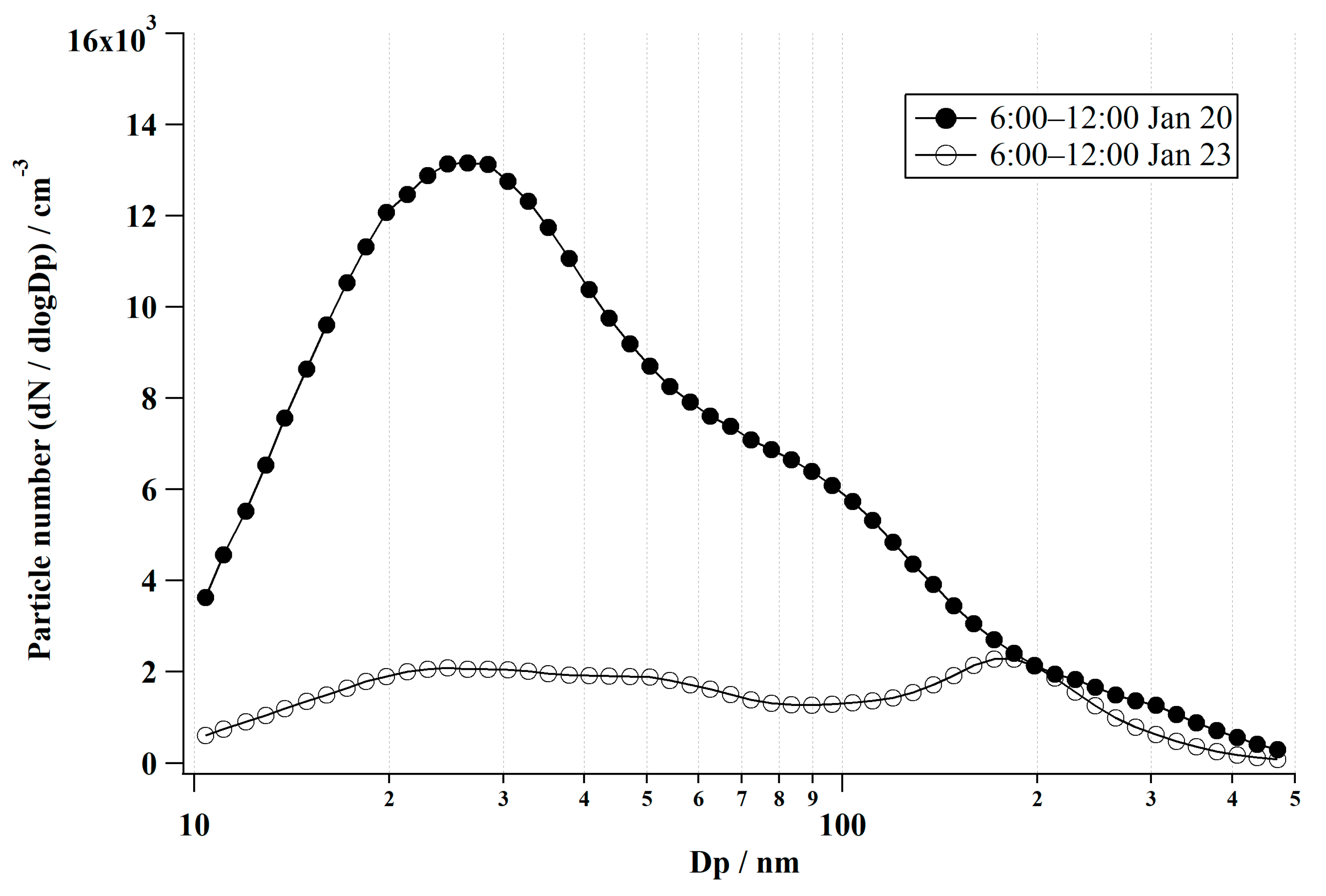
One of the highest PN concentrations in Group A was observed in the morning (6:00–12:00, 20 and 21 January). The PN of D_p was less than 50 nm, and was therefore considered to be very high (18.056 cm⁻³, 8:30 on 20 January). Figure 7 shows the particle size distribution measured using SMPS in the morning (6:00–12:00) on 20 and 23 January. The PN of D_p < 100 nm (ultrafine particles; UFPs) was much higher on 20 January in Group A (LAP, 13.126 cm⁻³ at D_p = 26.4 nm) than on 23 January in Group B (TAP, 2056 cm⁻³ at D_p = 26.4 nm). This was probably due to local emissions from car exhaust during rush hour and the accumulation of UFPs of D_p < than 100 nm due to the stagnant conditions caused by low wind speeds. Because of the winter season, an inversion layer may have formed during the night, causing the accumulation of air pollutants. Hasegawa et al. [25] measured roadside concentrations in Kawasaki City, Japan and found that particles with D_p = 30 nm disappeared after particles passed the thermal denuder at 250 °C. At this juncture, particles with D_p = 90 nm remained after thermal denuder treatment. Fushimi et al. [26] confirmed that particles with D_p = 30 nm consisted of volatile organic carbon from diesel vehicles, suggesting that the PN of UFP is due to local emissions from car exhaust which causes higher PN in the LAP. Thus, local emissions contribute to the increase in UFPs. The PN in the TAP period contains much fewer UFPs than that in the LAP period. During long-distance transport, the UFP particles probably coagulate and/or adsorb existing particles to form larger particles.

The PM_2.5 and the BC mass concentrations were also higher (PM_2.5: 12.5 μgm⁻³, BC: 410 ngm⁻³) in Group A (LAP) than in Group B (TAP) (PM_2.5: 9.1 μgm⁻³, BC: 230 ngm⁻³). Nitrate (NO₃⁻) concentrations showed a similar trend and were higher in Group A (LAP) (1.8 μgm⁻³) than in Group B (TAP) (0.8 μgm⁻³). NO₃⁻ was found in fine particles in the urban area; however, after long-distance transport, most NO₃⁻ was found in coarse particles [5]. The higher NO₃⁻ concentration observed in Group A (LAP) agreed with the variation in PN concentration and was considered to be of local origin. Car exhaust from the city is thought to be a primary source of BC, NO₃⁻, and PN.

4.3. Aging of Organics in PM

Positive matrix factorization (PMF) analysis was performed for the organics measured using Q-AMS. We used a PMF analysis method developed by Ulbrich et al. [21], and the interpretations followed previous results in the literature [22,23,24]. To evaluate the aging of organics, we adapted the two-factor analysis, because our purpose was to distinguish the TAP period from the LAP period. Factor 1 was low-volatile oxygenated organic aerosols (LV-OOA), which showed a distinctive mass peak at m/z = 44. Organics were well-aged. Observations in Group B (TAP) were expected. Factor 2 included semi-volatile oxygenated organic aerosols (SV-OOA) and hydrocarbon-like organic aerosols (HOA) [15,21,24,27,28]. Organics were not well-aged and were expected in group A (LAP).

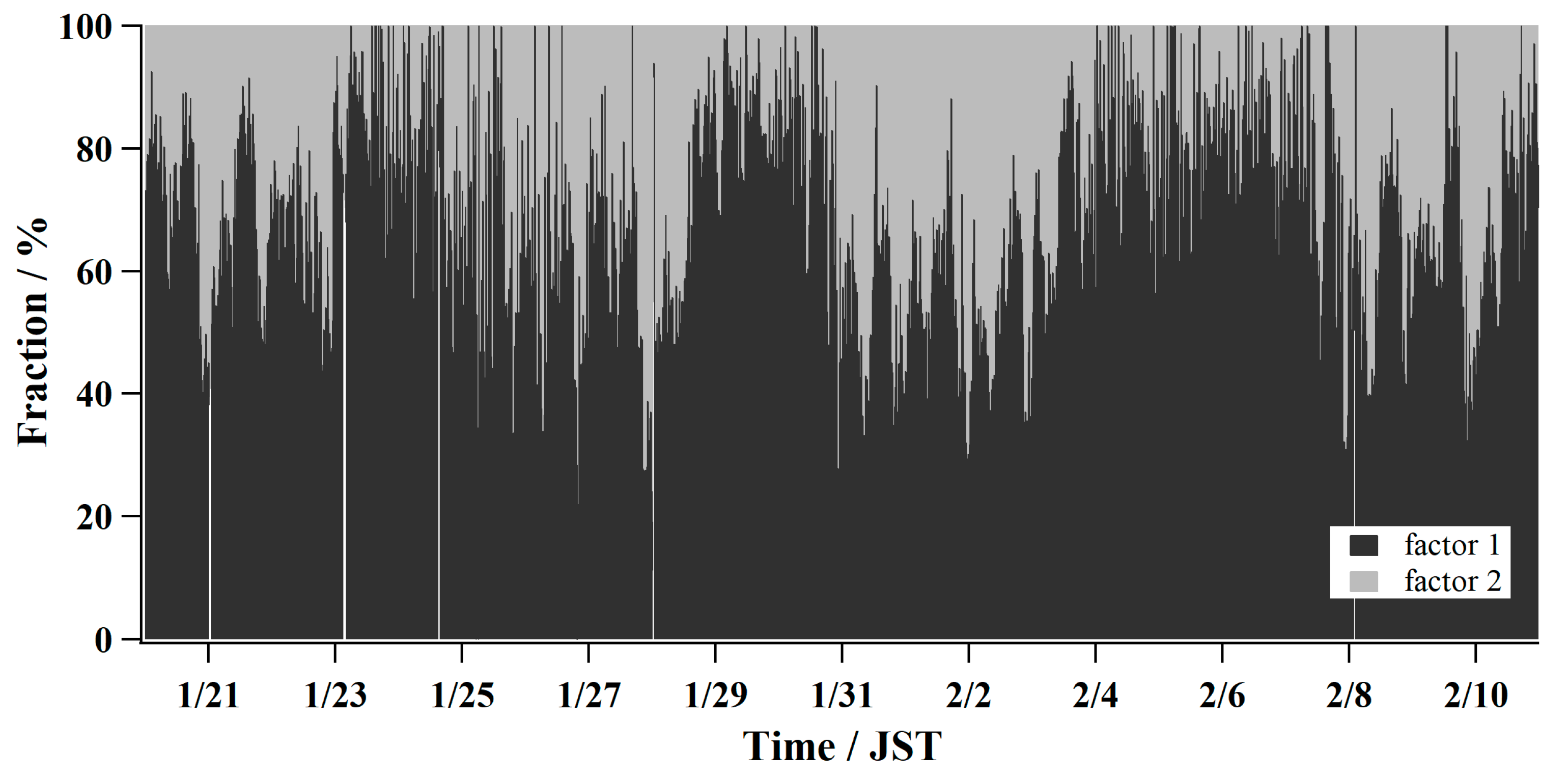
The fractions of Factor 1 and Factor 2 are shown in Figure 8. As expected, Factor 1 (LV-OOA) was dominant in group B (TAP). The fractions of Factor 1 and Factor 2 in TAP were 66% and 34%, respectively. The fraction of Factor 2 increased in Group A (LAP) and reached 44%, compared to that of 34% in TAP.

As the air mass was transported from the Asian continent, the aging time for organics was sufficient in Group B (TAP). However, the aging time in Group A (LAP) was insufficient to oxidize organic matter, because organics were emitted locally. These results are similar to those of previous PMF analysis of organics in Fukuoka [4], in which OOA reached 63% and 42% in the TAP and LAP periods, respectively. These PMF results agreed with the classifications of Group A (LAP) and Group B (TAP) based on wind speed.

Factor 1 for LV-OOA was 56% in LAP, indicating that more than half of the organics were aged. Organics were chemically transformed during transport in the atmosphere and changed to different molecules from the emitted volatile, organic carbon. Investigating the various toxicological adverse health effects of aged (LV-OOA) and fresh (HOA and SV-OOA) may be necessary.

4.4. LAP and TAP Features and Air Pollution Reduction

Based on the wind speed, the measurement period was clearly classified into two distinctive groups: Group A (LAP) and Group B (TAP). The gas and PM data supported the classification described above. In this study, the air pollutants (except ozone) were high in Group A (LAP) and low in Group B (TAP), indicating the importance of reducing local emissions to maintain better air quality in Fukuoka.

However, the average ozone concentrations remained at 36.4 ppb ± 5.41, and ozone variation was relatively small, even at night in Group B (TAP) than in Group A (LTP, 23.5 ppb ± 13.5). This finding indicates that ozone was produced outside the city and transported from the Asian continent. Recently, Chatani et al. [8] investigated the contribution of ozone from outside Japan using sensitivity and source apportion methods. Their analysis showed that most of the ozone was transported from China. Thus, reducing emissions across the wider region, including in China, is also important. Recently, PM_2.5 concentrations over 35 μg m⁻³ have seldom been reported in the Fukuoka area due primarily to PM reduction in China. This provides a good example of regional air quality achievements and indicates the importance of reducing emissions and improving air quality on a regional scale.

We have found that the air quality in Fukuoka is determined principally by local pollution with low wind speed; however, the ozone concentration is determined principally by transboundary air pollution. This finding indicates the following:

(1)

It is important for the local emission reduction to reduce PM and NOx.

(2)

However, it is important for regional emission reduction including China to reduce ozone.

The current study found that the region with the ability to reduce PM and ozone is different, which is an important finding to address ways of improving air quality.

5. Conclusions

We measured gaseous species and PM in Fukuoka, Japan, during the winter season of 2018. Because Fukuoka is located on the west side of Japan, transboundary air pollution (TAP) and local air pollution (LAP) influence the air quality. Thus, understanding the contributions of LAP and TAP is necessary to improve the air quality in Fukuoka.

We classified the measurement period into two distinct periods (LAP and TAP) based on wind speed. This classification is supported by the concentration variations of the gaseous species and by backward trajectories. We found that all air pollutants, except ozone, were high in the LAP period and low in the TAP period. The PN concentration was high in the LAP period because of the high UFP concentration from car exhaust during the morning rush hour. This was also supported by the higher concentrations of BC and NO₃⁻ in the LAP period. Although the formation of an inversion layer may cause the accumulation of air pollutants, our results show that it is important for reducing local emissions.

Ozone was higher in the TAP period, and the variations in ozone concentration were relatively small, indicating that ozone was produced outside the city and transported from the Asian continent. The PMF analysis revealed that the fractions of OOA (Factor 1) and Factor 2 in the TAP period were 66% and 34%, respectively. Thus, organics in PM are well-oxygenated (aged) in the TAP period because of sufficient aging time during long-range transport. Therefore, air pollutants must be reduced locally and regionally.

We found that the air quality in Fukuoka is determined principally by local pollution with low wind speed; however, the ozone concentration is determined principally by transboundary air pollution. This finding indicates the following:

(1)

It is important for local emission reduction to reduce PM and NOx;

(2)

However, it is also important for regional emission reduction including China to reduce ozone.

The authors believe that this study yields a very important finding, as it may contribute to improving air quality.