
Wintertime Cold Extremes in Northeast China and Their Linkage with Sea Ice in Barents-Kara Seas


Abstract
:1. Introduction
2. Data and Methods
3. Results
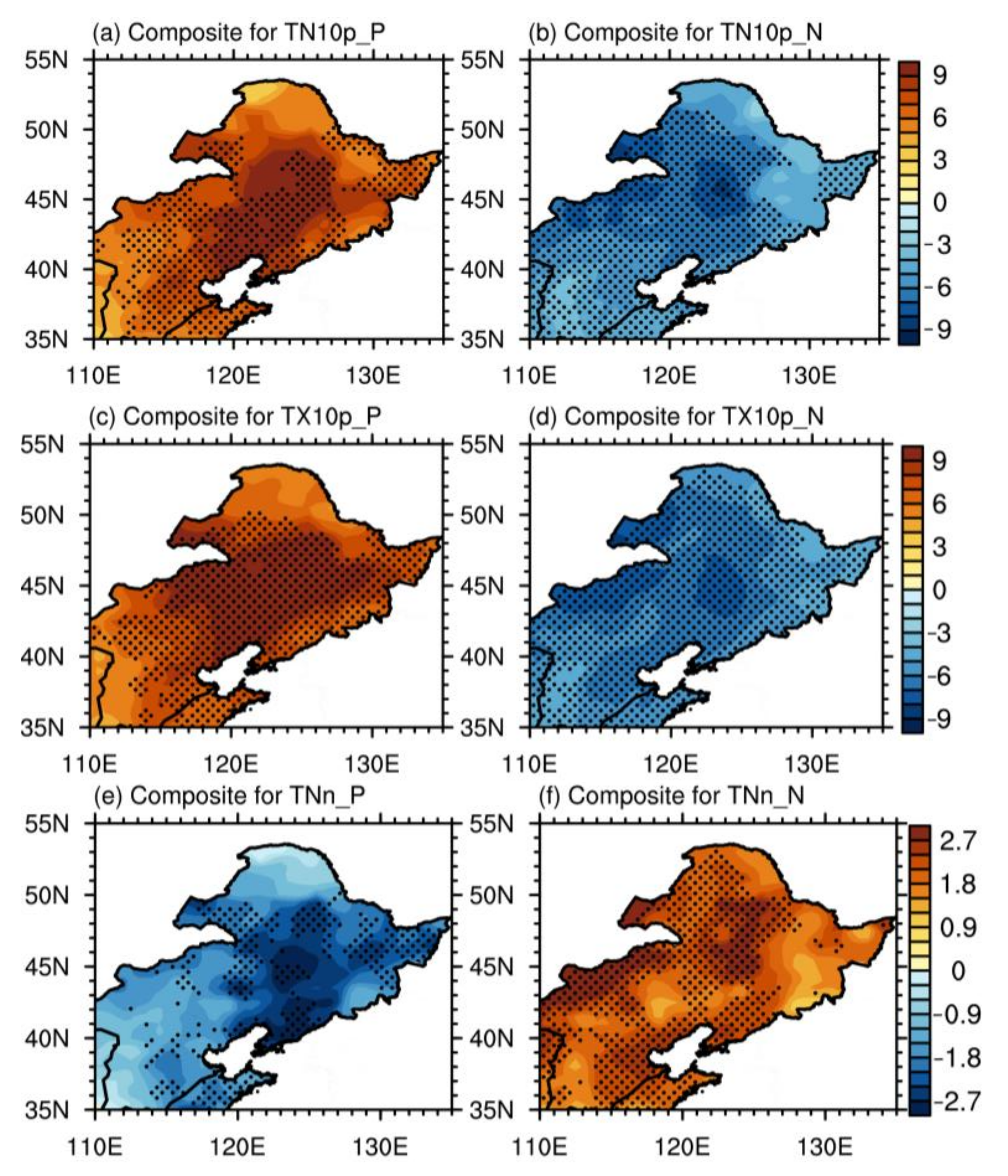
3.1. Spatial and Temporal Characteristics of WELT in NEC
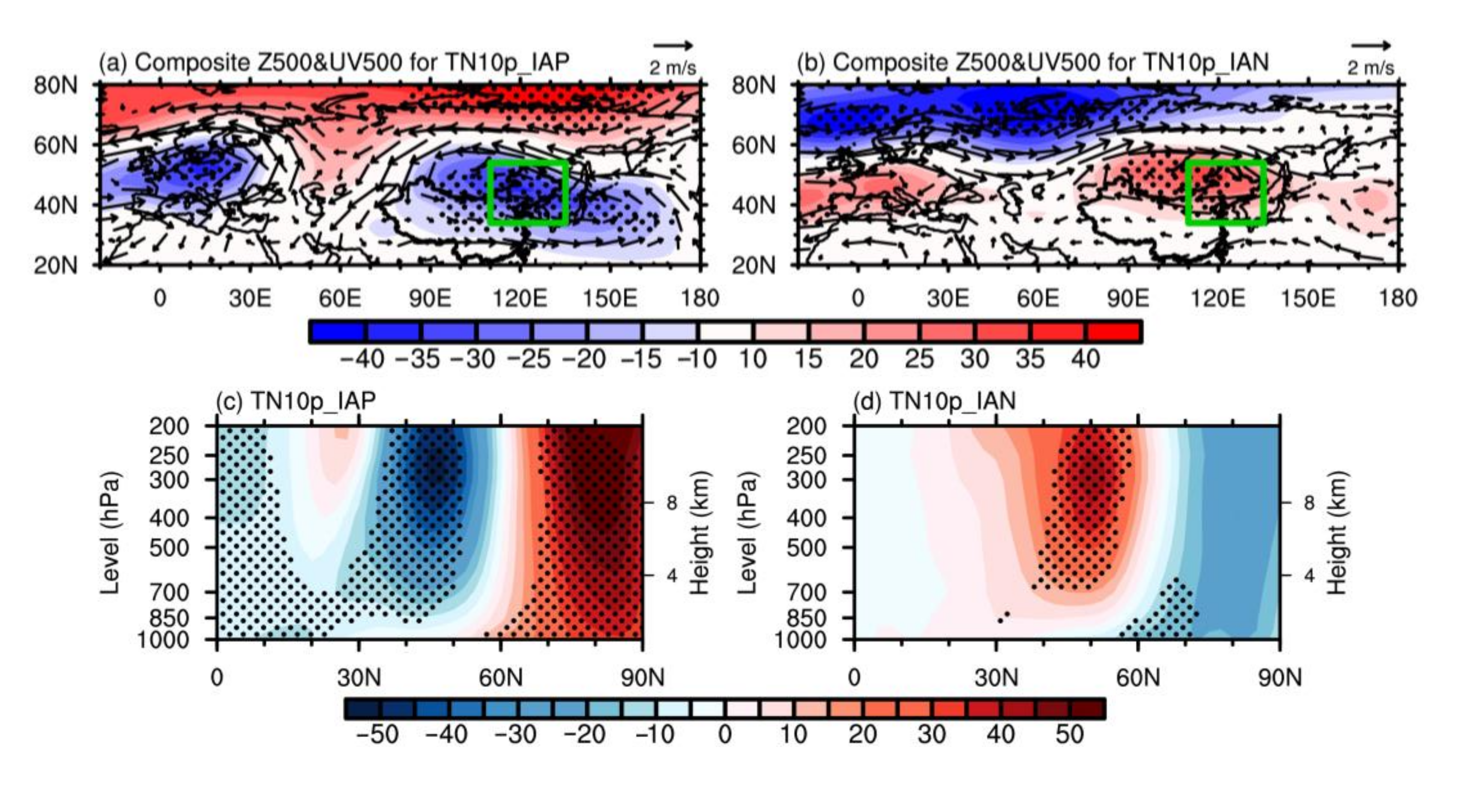
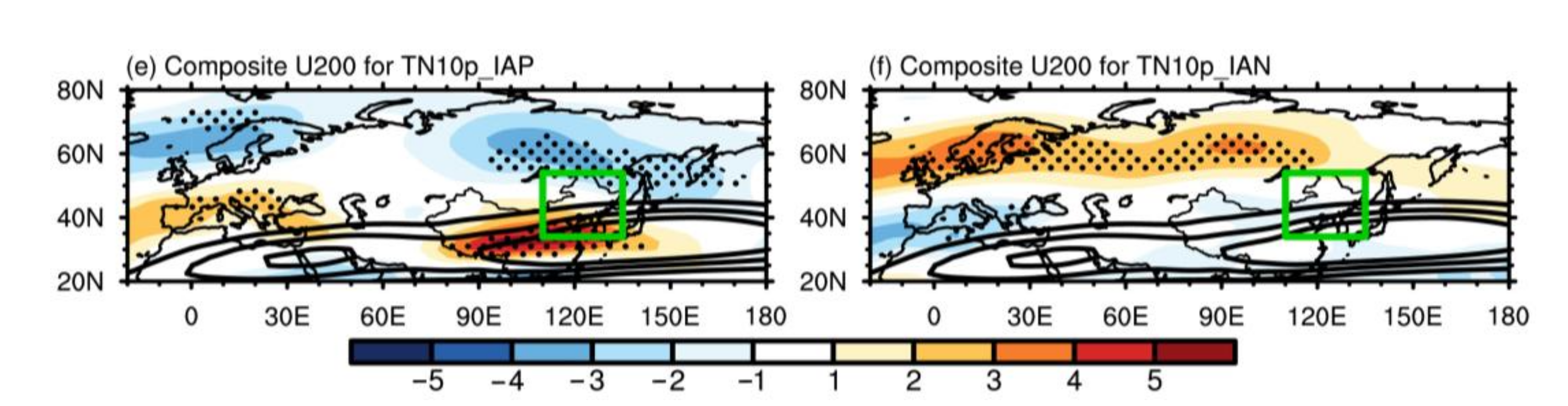
3.2. Atmospheric Circulation Patterns Affecting WELT in NEC
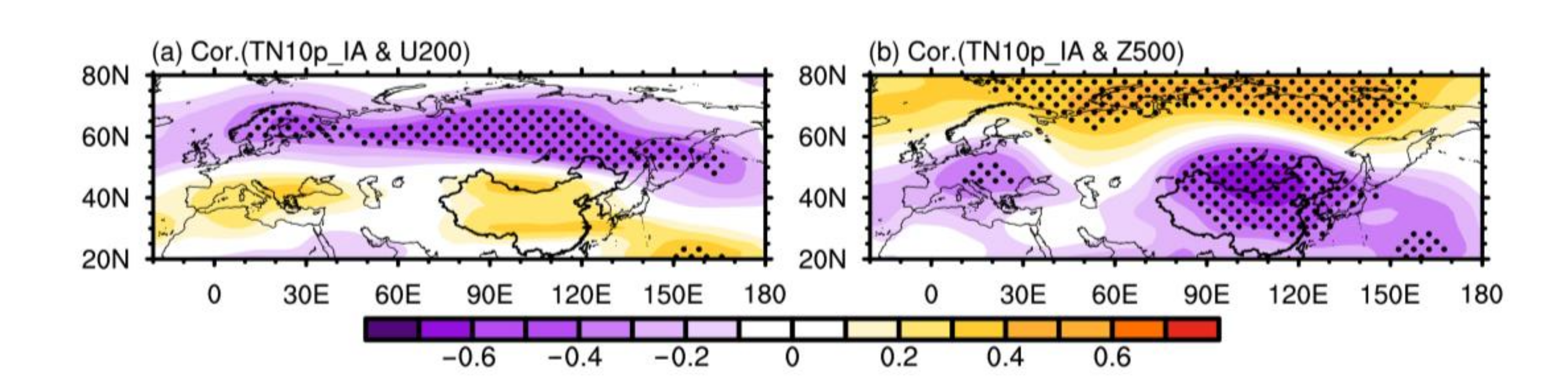
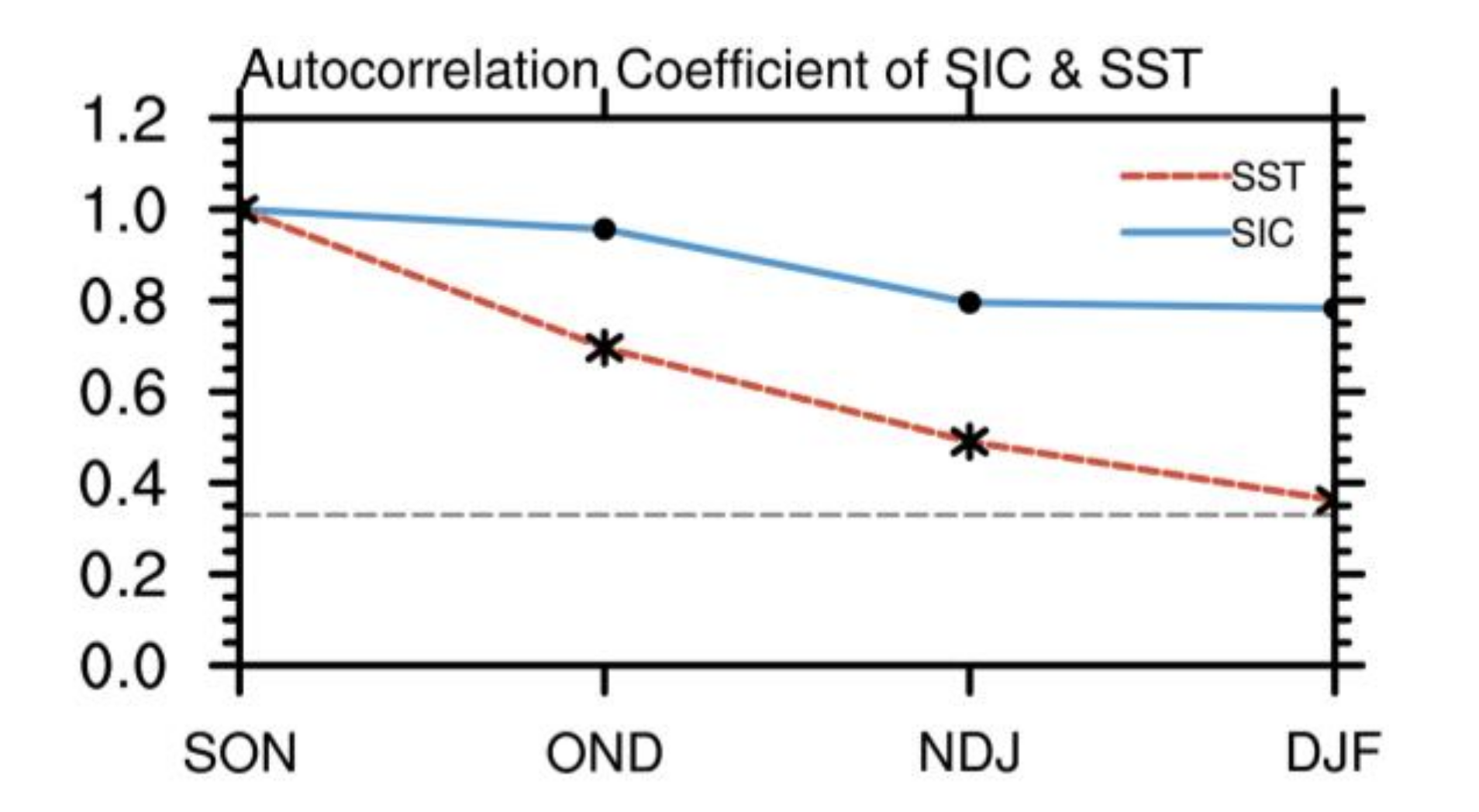
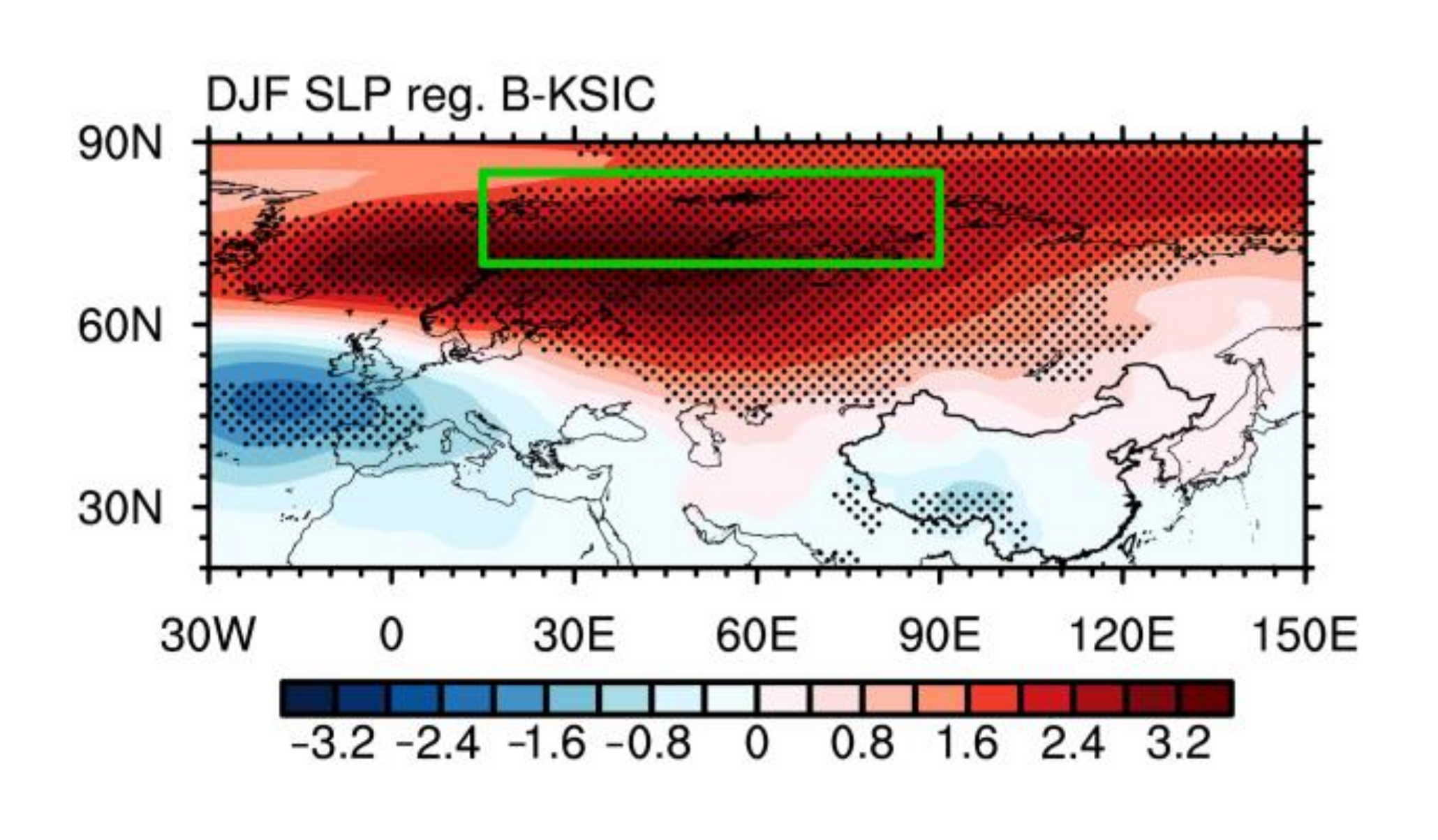
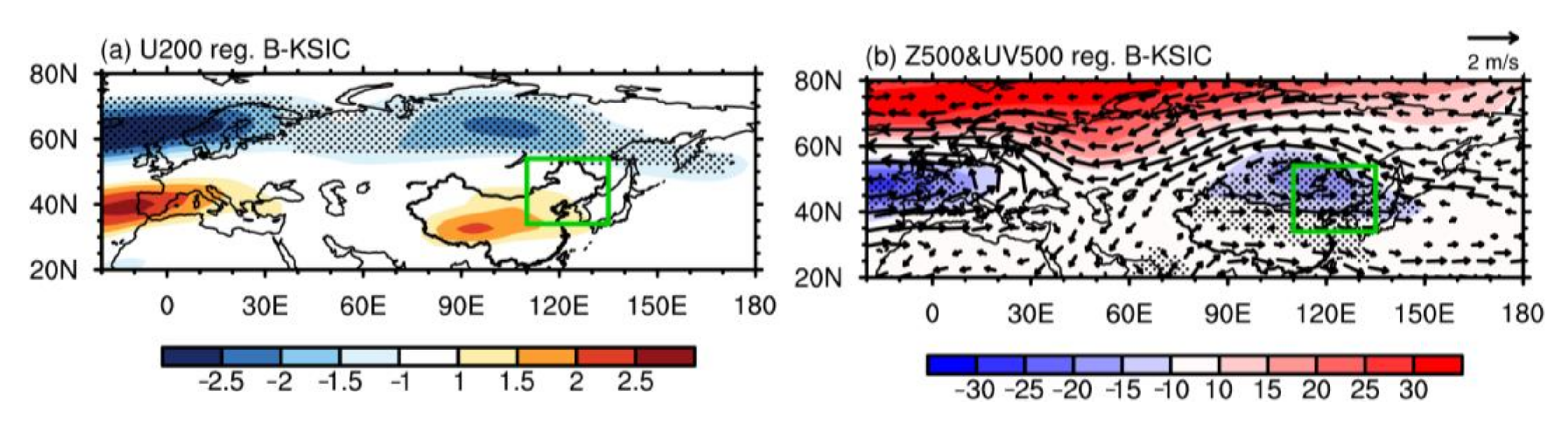
3.3. Effects of Arctic Sea Ice on Atmospheric Circulation Affecting the WELT in NEC
4. Conclusions and Discussion
Author Contributions
Funding
Institutional Review Board Statement
Informed Consent Statement
Acknowledgments
Conflicts of Interest
References
- Shen, Z.C.; Ren, G.Y.; Li, J.; Sun, X.B. Winter temperature variability and its relationship with atmospheric circulation anomalies in Northeast China. J. Meteorol. Environ. 2013, 29, 47–54. [Google Scholar]
- Li, C.; Fang, Z.H. Linkage of arctic oscillation and winter temperature in northeast China. Plateau Meteorol. 2005, 24, 927–934. [Google Scholar]
- Wu, B.Y.; Su, J.Z.; Zhang, R.H. Effects of autumn-winter Arctic sea ice on winter Siberian High. Chin. Sci. Bull. 2011, 56, 3220–3228. [Google Scholar] [CrossRef] [Green Version]
- Chen, P.Y.; Ni, Y.Q.; Yin, Y.H. Diagnostic study on the impact of the global sea surface temperature anomalies on the winter temperature anomalies in eastern China in past 50 years. J. Trop. Meteorol. 2001, 17, 371–380. [Google Scholar]
- Yang, S.Y.; Wang, Q.Q.; Sun, F.H. The winter air temperature anomalies and the changes of the atmosphere circulation characteristics in southern northeast China. J. Appl. Meteor. Sci. 2005, 16, 334–344. [Google Scholar]
- Honda, M.; Inoue, J.; Yamane, S. Influence of low Arctic sea-ice minima on anomalously cold Eurasian winters. Geophys. Res. Lett. 2009, 36, 1–7. [Google Scholar] [CrossRef]
- Wallace, J.M.; Smith, C.; Bretherton, C.S. Singular value de-composition of wintertime sea surface temperature and 500-mb height anomalies. J. Clim. 1992, 5, 561–576. [Google Scholar] [CrossRef]
- Bretherton, C.S.; Smith, C.; Wallace, J.M. An intercomparison of methods for finding coupled patterns in climate data. J. Clim. 1992, 5, 541–560. [Google Scholar] [CrossRef] [Green Version]
- Kumar, A.; Perlwitz, J.; Eischeid, J.; Quan, X.; Xu, T.; Zhang, T.; Hoerling, M.; Jha, B.; Wang, W. Contribution of sea ice loss to Arctic amplification. Geophys. Res. Lett. 2010, 37, 2–7. [Google Scholar] [CrossRef] [Green Version]
- Screen, J.A.; Simmonds, I. The central role of diminishing sea ice in recent Arctic temperature amplification. Nature 2010, 464, 1334–1337. [Google Scholar] [CrossRef] [Green Version]
- Alexander, M.A.; Bhatt, U.S.; Walsh, J.E.; Timlin, M.S.; Miller, J.S.; Scott, J.D. The atmospheric response to realistic Arctic sea ice anomalies in an AGCM during winter. J. Clim. 2004, 17, 890–905. [Google Scholar] [CrossRef] [Green Version]
- Honda, M.; Yamazaki, K.; Nakamura, H.; Takeuchi, K. Dynamic and thermodynamic characteristics of atmospheric response to anomalous sea-ice extent in the Sea of Okhotsk. J. Clim. 1999, 12, 3347–3358. [Google Scholar] [CrossRef]
- Mori, M.; Watanabe, M.; Shiogama, H.; Inoue, J.; Kimoto, M. Robust Arctic sea-ice influence on the frequent Eurasian cold winters in past decades. Nat. Geosci. 2014, 7, 869–873. [Google Scholar] [CrossRef]
- Screen, J.A.; Deser, C.; Sun, L.T. Reduced risk of North American cold extremes due to continued Arctic sea ice loss. Bull. Amer. Meteor. Soc. 2015, 96, 1489–1503. [Google Scholar] [CrossRef] [Green Version]
- Ma, S.M.; Zhu, C.W.; Liu, B.Q.; Zhou, T.J.; Ding, Y.H.; Orsolini, Y.J. Polarized response of east asian winter temperature extremes in the era of arctic warming. J. Clim. 2018, 31, 5543–5557. [Google Scholar] [CrossRef]
- Ma, S.M.; Zhu, C.W. Extreme cold wave over East Asia in January 2016: A possible response to the larger internal atmospheric variability induced by Arctic warming. J. Clim. 2019, 32, 1203–1216. [Google Scholar] [CrossRef]
- Petoukhov, V.; Semenov, V.A. A link between reduced Barents-Kara sea ice and cold winter extremes over northern continents. J. Geophys. Res. Atmos. 2010, 115, 1–11. [Google Scholar] [CrossRef]
- Wu, Q.; Zhang, X. Observed forcing-feedback processes between Northern Hemisphere atmospheric circulation and Arctic sea ice coverage. J. Geophys. Res. Atmos. 2010, 115, 1–9. [Google Scholar] [CrossRef]
- Inoue, J.; Hori, M.E.; Takaya, K. The role of barents sea ice in the wintertime cyclone track and emergence of a warm-Arctic cold-Siberian anomaly. J. Clim. 2012, 25, 2561–2569. [Google Scholar] [CrossRef]
- Liu, J.; Curry, J.; Wang, H.; Song, M.; Horton, R.M. Impact of declining Arctic sea ice on winter snowfall. Proc. Natl. Acad. Sci. USA 2012, 109, 4074–4079. [Google Scholar] [CrossRef] [Green Version]
- Cohen, J.L.; Furtado, J.C.; Barlow, M.A.; Alexeev, V.A.; Cherry, J.E. Arctic warming, increasing snow cover and widespread boreal winter cooling. Environ. Res. Lett. 2012, 7, 014007. [Google Scholar] [CrossRef]
- Cohen, J. An observational analysis: Tropical relative to Arctic influence on midlatitude weather in the era of Arctic amplification. Geophys. Res. Lett. 2016, 43, 5287–5294. [Google Scholar] [CrossRef]
- Ma, S.M.; Zhu, C.W. Opposing trends of winter cold extremes over eastern eurasia and north america under recent Arctic warming. Adv. Atmos. Sci. 2020, 37, 1417–1434. [Google Scholar] [CrossRef]
- Walsh, J.E.; Chapman, W.L.; Fetterer, F. Gridded monthly sea ice extent and concentration, 1850 onwards, Version 1.1. Boulder, Colorado USA: National Snow and Ice Data Center. Digital Media 2016. [Google Scholar] [CrossRef]
- Kalnay, E.; Kanamitsu, M.; Kistler, R.; Collins, W.; Deaven, D.; Gandin, L.; Iredell, M.; Saha, S.; White, G.; Woollen, J.; et al. The NCEP/NCAR 40-year reanalysis project. Bull. Am. Meteorol. Soc. 1996, 77, 437–472. [Google Scholar] [CrossRef] [Green Version]
- You, Q.L.; Ren, G.Y.; Fraedrich, K.; Kang, S.C.; Ren, Y.Y.; Wang, P.L. Winter temperature extremes in China and their possible causes. Int. J. Clim. 2013, 33, 1444–1455. [Google Scholar] [CrossRef]
- You, Q.L.; Kang, S.C.; Aguilar, E.; Pepin, N.; Fluegel, W.A.; Yan, Y.P. Changes in daily climate extremes in China and their connection to the large scale atmospheric circulation during 1961–2003. Clim. Dyn. 2011, 36, 2399–2417. [Google Scholar] [CrossRef]
- Meehl, G.A.; Tebaldi, C. More intense, more frequent, and longer lasting heat waves in the 21st century. Science 2004, 305, 994–997. [Google Scholar] [CrossRef] [Green Version]
- An, X.D.; Sheng, L.F.; Liu, Q.; Li, C.; Gao, Y.; Li, J.P. The combined effect of two westerly jet waveguides on heavy haze in the North China Plain in November and December 2015. Atmos. Chem. Phy. 2020, 20, 4667–4680. [Google Scholar] [CrossRef] [Green Version]
- Shi, J.; Wu, K.; Qian, W.; Huang, F.; Li, C.; Tang, C. Characteristics, trend, and precursors of extreme cold events in northwestern North America. Atmos. Res. 2021, 249, 105338. [Google Scholar] [CrossRef]
- Sun, J.Q. Record-breaking SST over mid-North Atlantic and extreme high temperature over the Jianghuai–Jiangnan region of China in 2013. Chin. Sci. Bull. 2014, 59, 3465–3470. [Google Scholar] [CrossRef]
- Xu, X.P.; He, S.P.; Gao, Y.Q.; Furevik, T.; Wang, H.J.; Li, F.; Ogawa, F. Strengthened linkage between midlatitudes and Arctic in boreal winter. Clim. Dyn. 2019, 53, 3971–3983. [Google Scholar] [CrossRef]
- Kim, B.M.; Son, S.W.; Min, S.K.; Jeong, J.H.; Kim, S.J.; Zhang, X.D.; Shim, T.; Yoon, J.H. Weakening of the stratospheric polar vortex by Arctic sea-ice loss. Nat. Comm. 2014, 5, 4646. [Google Scholar] [CrossRef] [PubMed] [Green Version]


| Acronym | Indicator | Definitions | Unit |
|---|---|---|---|
| TN10p | Cold nights | Days when daily minimum temperature is smaller than the 10th percentile threshold in winter | days |
| TX10p | Cold days | Days when daily maximum temperature is smaller than the 10th percentile threshold in winter | days |
| TNn | Coldest temperature | The minimum temperature of daily minimum temperature in winter | °C |
| Phase | Years | ||||||
|---|---|---|---|---|---|---|---|
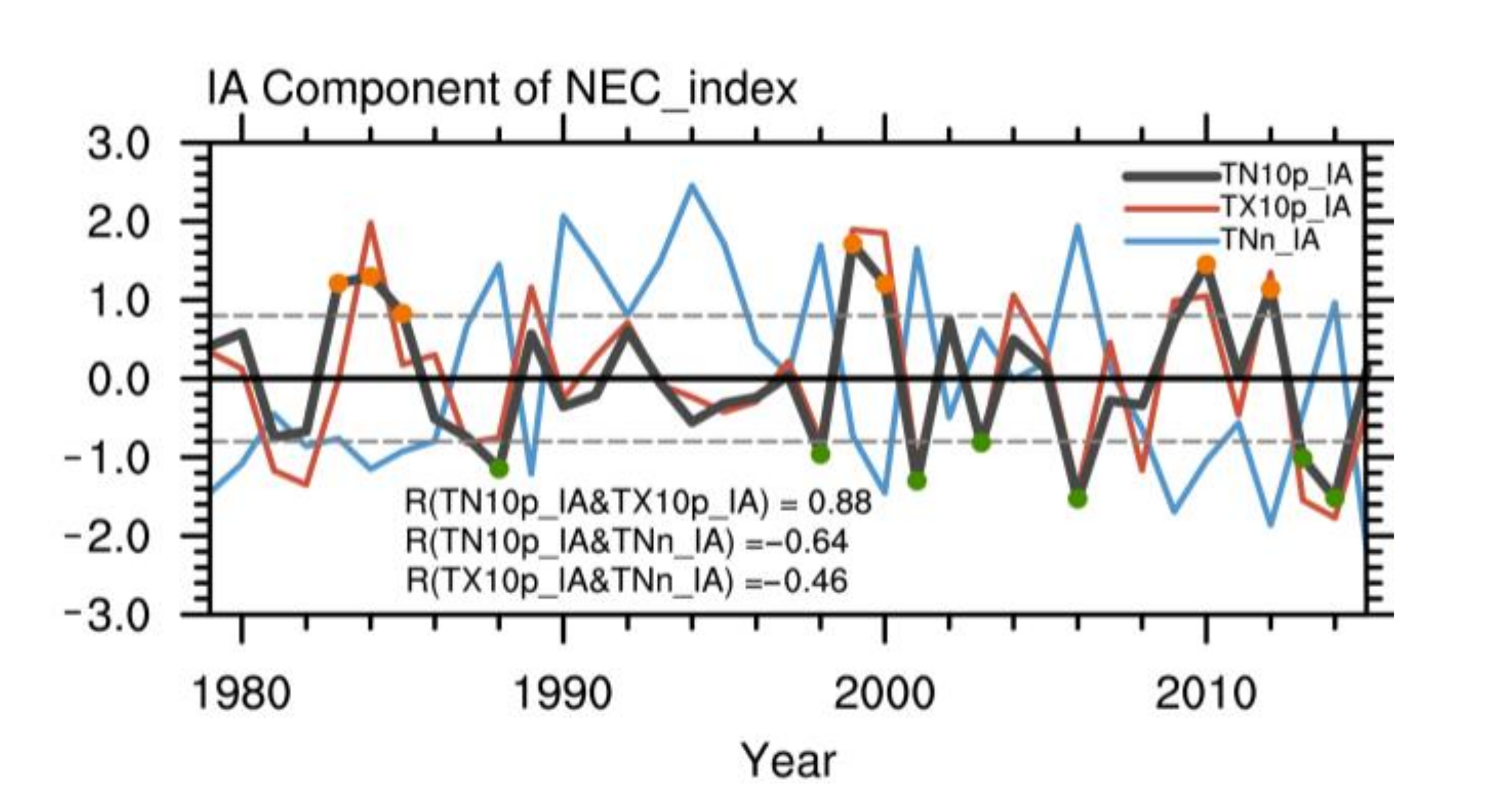
| TN10p_IAP | 1983 | 1984 | 1985 | 1999 | 2000 | 2010 | 2012 |
| TN10p_IAN | 1988 | 1998 | 2001 | 2003 | 2006 | 2013 | 2014 |
Publisher’s Note: MDPI stays neutral with regard to jurisdictional claims in published maps and institutional affiliations. |
© 2021 by the authors. Licensee MDPI, Basel, Switzerland. This article is an open access article distributed under the terms and conditions of the Creative Commons Attribution (CC BY) license (http://creativecommons.org/licenses/by/4.0/).
Share and Cite
Luo, Y.; Li, C.; Shi, J.; An, X.; Sun, Y. Wintertime Cold Extremes in Northeast China and Their Linkage with Sea Ice in Barents-Kara Seas. Atmosphere 2021, 12, 386. https://doi.org/10.3390/atmos12030386
Luo Y, Li C, Shi J, An X, Sun Y. Wintertime Cold Extremes in Northeast China and Their Linkage with Sea Ice in Barents-Kara Seas. Atmosphere. 2021; 12(3):386. https://doi.org/10.3390/atmos12030386
Chicago/Turabian StyleLuo, Yongyue, Chun Li, Jian Shi, Xiadong An, and Yaqing Sun. 2021. "Wintertime Cold Extremes in Northeast China and Their Linkage with Sea Ice in Barents-Kara Seas" Atmosphere 12, no. 3: 386. https://doi.org/10.3390/atmos12030386